10 Capital One Data Analyst Interview Questions & Answers

capital-one icon

Questions with Detailed ExplanationsWith Detailed Explanations

(Last Updated: September 13, 2026)

1. How would you persuade customers to switch from paper credit card statements to electronic statements?Data AnalysisMediumCapital One

Short Interview Answer (30-60 seconds)

I would first define the decision: which eligible paper-statement customers should receive which message or experience to encourage electronic-statement enrollment. I would define the conversion rate as customers who switch to electronic statements divided by eligible customers exposed to the opportunity, over a clearly defined window. Then I would analyze the current enrollment funnel and segment customers by relevant observed behavior or account characteristics, without assuming why they prefer paper. I would identify likely friction points, test targeted benefit-focused messages or a simpler enrollment experience through a controlled experiment where possible, and measure incremental conversion along with guardrails such as opt-outs, complaints, failed enrollment, and later reversions to paper.

Detailed Explanation

The goal is not simply to tell customers that electronic statements are better. The task is to understand why eligible customers still use paper, identify where they stop during the switch process, and choose actions that can increase electronic-statement adoption. I would begin by defining who is eligible, what counts as a successful switch, and the time period for measuring it. Then I would study customer behavior, compare meaningful groups, investigate barriers, test possible improvements, and measure whether the chosen action causes more customers to switch rather than only being associated with switching.

Useful Questions to Ask the Interviewer
  1. Which customers are eligible to receive electronic statements, and are any customers required to remain on paper?
  2. What business decision should this analysis support: communication strategy, enrollment-flow improvements, targeting, incentives, or a combination?
  3. What events are available for the enrollment journey, such as offer shown, enrollment started, verification completed, and electronic statements activated?
  4. What customer and account attributes may legally and appropriately be used for segmentation or targeting?
  5. What historical communication, enrollment, opt-out, complaint, or statement-preference data is available?
  6. Is there an existing experiment platform or control group that can measure incremental conversion?
  7. Which guardrail outcomes matter besides adoption, such as complaints, delivery problems, reversions to paper, or support contacts?
How to Explain It in an Interview

I would start with the business decision. The decision is not merely whether electronic statements are desirable. It is which action should be used for which eligible customers to increase voluntary electronic-statement adoption while maintaining a good customer experience.

First, I would define the population and unit of analysis. The population would be customers who currently receive paper statements and are eligible to switch. I would confirm whether the analysis should use one row per customer, account, or customer-account relationship, because a customer could potentially have more than one account. I would also define the observation window and make sure the same window is used when comparing groups.

Next, I would define the primary KPI before exploring the data. A useful primary metric is electronic-statement conversion rate: the number of eligible customers who successfully switch within the measurement window divided by the number of eligible customers who had the relevant opportunity to switch. The denominator matters. For example, customers who could not enroll should not silently be treated the same as customers who were eligible and chose not to enroll.

I would establish a baseline conversion rate and examine the current customer journey. A funnel analysis means measuring how many customers move through each important step. Depending on the available instrumentation, that might include being presented with an enrollment opportunity, starting enrollment, completing any required steps, and successfully activating electronic statements. I would not invent funnel stages that are not captured; I would first confirm which events actually exist.

The funnel helps separate different problems. If many eligible customers never begin enrollment, the issue may be awareness, message relevance, or channel reach. If customers frequently begin but do not complete enrollment, the larger opportunity may be reducing friction in the process. If activation succeeds but customers later return to paper, the issue may be satisfaction, access, notifications, or another post-enrollment concern. These are diagnostic possibilities, not conclusions until the data supports them.

I would then use segmentation analysis, which means comparing the same metric across meaningful customer groups. I would use only attributes that are available, appropriate, and permitted for the decision. Relevant dimensions could include observed digital engagement, communication channel, account relationship, prior response to statement-related communications, or other approved customer characteristics. I would compare both the conversion rate and the size of each segment, because a very high rate in a tiny group may have little business impact.

I would also examine trends or cohorts when they add information. For example, if customers exposed to different enrollment experiences at different times can be identified, cohort analysis can compare how their adoption and retention of the electronic preference develop over comparable periods. I would keep calendar effects and unequal follow-up windows in mind so that newer cohorts are not unfairly compared with older cohorts.

For root-cause investigation, I would drill down into where conversion differs and look for supporting evidence. I might compare funnel drop-off, communication exposure, failed enrollment events, repeated attempts, support interactions, or other available signals. I would check whether apparent patterns could instead come from missing data, changes in instrumentation, different eligibility rules, or differences in the customers who received each experience.

I would be careful not to treat correlation as proof of cause. Suppose digitally active customers have a higher electronic-statement adoption rate. That observation does not prove that sending customers more digital messages will cause them to switch. Those customers may already be more comfortable with online services. Descriptive analysis tells me what happened, diagnostic analysis helps investigate why it may have happened, and causal evidence is needed before claiming that a specific intervention produced the change.

Once the main barriers are understood, I would move to prescriptive actions. The intervention should match the diagnosed problem. If awareness appears to be the issue, I might test clear benefit-focused communication with an easy path to enrollment. The message could explain relevant benefits that the business can support, rather than making unsupported claims. If the funnel shows abandonment during enrollment, I would prioritize simplifying the process before increasing message volume. If different segments respond differently, I would test appropriately tailored experiences rather than assume one message is best for everyone.

Where feasible, I would use a randomized controlled experiment. Eligible customers would be randomly assigned to a control experience and one or more treatment experiences. Treatments might compare message framing, communication channels, enrollment-flow changes, or another approved intervention. The primary outcome would be the predefined electronic-statement conversion rate over the same window. Random assignment helps separate the treatment effect from pre-existing customer differences. I would determine the sample-size requirement and experiment duration before reading the results rather than stopping as soon as one variant appears better.

I would also define guardrails. Increasing enrollment is not enough if the approach produces unacceptable complaints, opt-outs, unsuccessful delivery, support burden, or rapid reversion to paper. The exact guardrails should be agreed with the business before the test. If incentives are considered, I would also compare incremental adoption with the incentive and program costs rather than looking only at conversion.

Before trusting any result, I would validate the data. I would check eligibility logic, duplicate customer or account records, missing preference values, freshness of enrollment events, inconsistent timestamps, unusual spikes, and whether the numerator can accidentally contain records outside the denominator. I would reconcile key counts against a trusted source when one exists and verify that treatment and control assignment was implemented as intended.

I would also consider uncertainty. Small segments can show large apparent differences by chance, some customer actions may be incompletely observed, and operational changes during the test can affect results. I would report uncertainty at a level appropriate to the analysis and avoid presenting a small or unstable difference as a guaranteed business impact.

Finally, I would present the recommendation in decision language. I would state which intervention performed better, for which eligible population, what uncertainty remains, and whether the evidence supports rollout, further testing, or no change. I would continue measuring electronic-statement adoption after rollout and monitor guardrails and reversions. If later evidence shows that the effect disappears, customer experience worsens, or the result does not reproduce, I would revise the recommendation rather than defend the original conclusion.

Technical Approach
  1. Define the business decision and decision owner.
  2. Confirm the eligible paper-statement population and the correct unit of analysis.
  3. Define electronic-statement conversion rate, denominator, measurement window, baseline, and guardrails before exploring results.
  4. Validate eligibility, statement-preference, communication, funnel-event, and outcome data for missingness, duplicates, freshness, and inconsistent records.
  5. Describe the current adoption rate and enrollment funnel to locate major drop-off points.
  6. Segment the same metrics across meaningful and permitted customer dimensions, checking both segment rates and segment sizes.
  7. Investigate likely barriers using available behavioral and funnel evidence while keeping assumptions separate from findings.
  8. Distinguish correlations from causal claims and identify alternative explanations for observed differences.
  9. Design interventions that directly address the observed barrier, such as clearer benefit-focused communication or lower enrollment friction.
  10. Where feasible, randomly test interventions against a control using a predefined outcome window, sample plan, and guardrails.
  11. Compare incremental conversion, uncertainty, customer-experience effects, and relevant costs.
  12. Recommend rollout, further testing, or no change based on the strength of the evidence, then monitor adoption and reversions after the decision.
Practical Insights

The main cost is usually not the calculation itself but collecting trustworthy customer, eligibility, communication, and enrollment data and running a test long enough to make a reliable decision. Simple funnel and segment summaries are relatively easy to compute, but many segments can create noisy comparisons and false patterns. Experiments require enough eligible customers and time to detect a meaningful difference. More personalized targeting may improve relevance, but it adds operational, governance, interpretability, and maintenance costs. A simpler intervention is preferable when it produces similar evidence of improvement with fewer risks.

Why Interviewers Ask This

This question tests whether the candidate can turn a broad customer-behavior problem into a measurable business decision. A strong answer should define the target population and conversion metric, identify meaningful customer segments and barriers, distinguish observed associations from causal evidence, propose proportionate interventions, and explain how to measure whether those interventions actually increase electronic-statement adoption without creating unacceptable customer-experience or operational problems.

Common interview mistakes

Common mistakes include immediately proposing discounts or repeated reminders without first identifying the barrier; using all paper-statement customers as the denominator without checking eligibility; discussing conversion without defining the measurement window; comparing segments without considering their size or different exposure opportunities; assuming digitally engaged customers prove that digital messaging causes adoption; inventing customer motivations that are not supported by data; ignoring customers who start but fail to complete enrollment; declaring success from a higher raw conversion rate without a valid control or comparable baseline; stopping an experiment early because one treatment temporarily looks better; and optimizing adoption while ignoring complaints, opt-outs, reversions, costs, or other guardrails.

Interview tip

Structure the answer as a decision problem: define eligible customers and conversion first, diagnose the funnel and segments second, test a targeted intervention third, and finish with causal measurement and guardrails. Avoid claiming that you already know why customers prefer paper; show how the data would distinguish possible explanations.
Interviewer may ask next
What would you do if customers who are already highly active in digital channels have much higher electronic-statement adoption?

I would treat that as a useful descriptive finding, not evidence that increasing digital engagement will cause electronic-statement adoption. I would first verify that both groups have the same eligibility definition, measurement window, and opportunity to enroll. Then I would examine whether the difference remains across relevant segments and funnel stages. The pattern could reflect comfort with digital products, different communication exposure, account characteristics, or another factor. If the business wants to know whether a specific digital message causes more adoption, I would test that intervention with random assignment where feasible and compare incremental conversion against a control.

What if a campaign increases electronic-statement enrollment but also increases customer complaints and later switches back to paper?

I would not judge the campaign on initial conversion alone. I would compare the incremental conversion with the predefined guardrails, including complaints and reversions, over an appropriate follow-up window. A campaign that creates short-term adoption but poor customer experience may not be a good business decision. I would investigate where the complaints or reversions are concentrated, determine whether the issue is the message, enrollment process, notification experience, or another supported factor, and test a less aggressive or better-targeted approach. The final recommendation should balance durable adoption with customer experience and relevant operational costs.

2. Capital One launches a pre-approved credit-line increase offer in its app. What north-star metric and four guardrails would you track during the first 30 days?Data AnalysisEasyCapital One

Question Details

Balance incremental business value against credit risk, customer harm, portfolio health, and operational cost. Define every metric precisely.

Short Interview Answer (30-60 seconds)

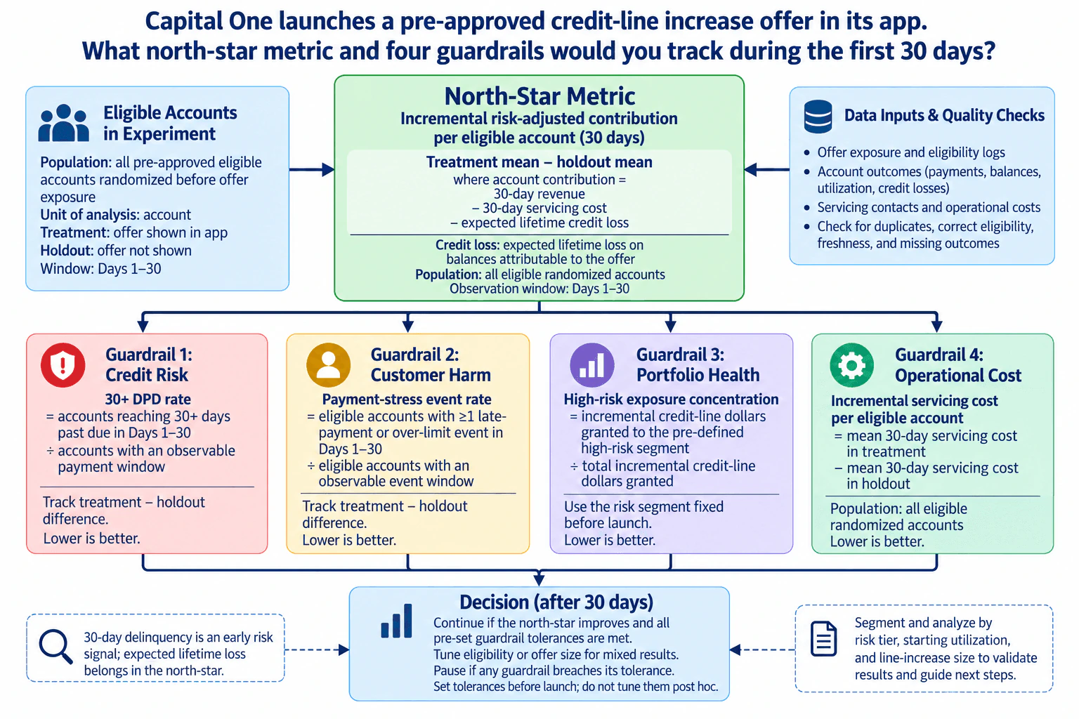
I would use incremental risk-adjusted contribution per eligible account as the north star. With eligible accounts randomized before exposure, I would calculate the treatment mean minus the holdout mean, where account contribution is 30-day revenue minus 30-day servicing cost minus expected lifetime credit loss on balances attributable to the offer. My four guardrails would be 30+ DPD rate, payment-stress event rate, high-risk exposure concentration, and incremental servicing cost per eligible account. I would set tolerances before launch, monitor treatment-versus-holdout differences, segment by risk tier, utilization, and line-increase size, and continue, tune, or pause after 30 days based on the combined result.

Detailed Explanation

The task is to decide whether a pre-approved credit-line increase offer creates enough incremental business value to justify its risks and costs during the first 30 days. I would not judge the launch only by acceptance, spending, or revenue. I would compare randomized eligible accounts that see the offer with eligible holdout accounts that do not. The main KPI should combine revenue, servicing cost, and expected credit loss. Then I would watch four separate guardrails for credit risk, customer harm, portfolio concentration, and operational cost before deciding whether to continue, adjust, or pause the rollout.

Useful Questions to Ask the Interviewer
  1. Are eligible accounts randomized into treatment and holdout before the offer is shown?
  2. What exact revenue components should count in the contribution metric?
  3. What approved expected-credit-loss methodology should be used for balances attributable to the offer?
  4. What definitions are available for late-payment, over-limit, servicing-cost, risk-tier, and utilization fields?
  5. What guardrail tolerances will be approved before launch?
  6. Are there minimum sample-size or statistical-confidence requirements for the overall result and key segments?
Capital One launches a pre-approved credit-line increase offer in its app. What north-star metric and four guardrails would you track during the first 30 days? diagram
How to Explain It in an Interview

I would start with the business decision: after 30 days, should Capital One continue the rollout, change eligibility or offer size, or pause it? To answer that, I would define the experiment and every KPI before looking at results.

The population is all pre-approved eligible accounts that are randomized before offer exposure. The unit of analysis is the account. Treatment accounts are shown the offer in the app, while holdout accounts are not shown the offer. The primary observation window is Days 1 through 30. Randomization matters because a treatment-minus-holdout difference can support a causal interpretation when assignment, exposure, and measurement remain valid.

My north-star metric is incremental risk-adjusted contribution per eligible account. First calculate an account-level contribution for each randomized account:

account contribution = 30-day revenue − 30-day servicing cost − expected lifetime credit loss on balances attributable to the offer.

Then calculate:

north-star = mean account contribution in treatment − mean account contribution in holdout.

Using all eligible randomized accounts keeps the denominator aligned with the product decision and avoids making the KPI look better simply because only people who accepted the increase are included. The 30-day period is the observation window for launch activity, while the expected credit-loss component reflects the expected lifetime loss associated with balances attributable to the offer. That distinction matters because the full credit-loss lifecycle will not be observed within 30 days.

I would then monitor four guardrails.

  1. Credit risk — 30+ DPD rate. Define it as accounts reaching at least 30 days past due during Days 1–30 divided by accounts with an observable payment window. I would track the treatment-minus-holdout difference. Lower is better. This is an early risk signal, not a substitute for the lifetime expected loss included in the north star.
  1. Customer harm — payment-stress event rate. Define it as eligible accounts with at least one late-payment or over-limit event during Days 1–30 divided by eligible accounts with an observable event window. I would track the treatment-minus-holdout difference, with lower being better. This captures adverse customer behavior that may appear before a full credit-loss outcome develops.
  1. Portfolio health — high-risk exposure concentration. Define the numerator as incremental credit-line dollars granted to a pre-defined high-risk segment and the denominator as total incremental credit-line dollars granted. The risk segment must be fixed before launch rather than chosen after seeing outcomes. Lower is better under this guardrail definition, but the actual decision should use the pre-set portfolio tolerance rather than an invented universal threshold.
  1. Operational cost — incremental servicing cost per eligible account. Define it as mean 30-day servicing cost in treatment minus mean 30-day servicing cost in holdout across all eligible randomized accounts. Lower is better because a program that creates value but also causes large incremental servicing costs may not scale economically.

Before interpreting any KPI, I would validate the inputs. I would reconcile eligibility and exposure logs, verify randomization counts, check that treatment accounts received the intended exposure, confirm holdout contamination is minimal, check duplicates, freshness, and missing outcomes, and confirm that account-level events are aggregated only once. For rate metrics, I would explicitly verify the observable-window denominator so accounts without enough follow-up are not incorrectly treated as non-events.

I would also review trends through the 30-day window instead of relying only on the final aggregate. A stable overall result can hide deterioration in a later cohort or subgroup. Segmentation analysis means calculating the same treatment-versus-holdout metrics across meaningful pre-defined dimensions. Here I would use risk tier, starting utilization, and line-increase size because those dimensions can reveal where value or harm is concentrated. I would be cautious with small groups because sparse segment estimates can be noisy, and many post-hoc cuts can create misleading patterns.

The causal claim should stay tied to randomization. If treatment and holdout were assigned randomly and the experiment remained clean, the treatment-minus-holdout difference is the main evidence for incremental impact. A simple correlation such as customers who accepted the increase spending more would not be enough because customers who accept may already differ from customers who do not.

There are also timing and measurement limitations. Thirty days may be enough to observe revenue, servicing activity, payment stress, and early delinquency signals, but it is too short to observe the full realized credit-loss lifecycle. That is why the north star uses expected lifetime credit loss attributable to the offer while the 30+ DPD guardrail is treated as an early indicator. Expected loss is still an estimate, so model uncertainty should be acknowledged and monitored.

The decision rule should be set before looking at results. Continue the rollout if the north-star metric improves and every guardrail remains within its pre-set tolerance. If the overall economics are positive but a segment or guardrail is weak, tune eligibility or line-increase size and measure again. If a material guardrail breaches its tolerance, pause or restrict the rollout even if short-term contribution looks attractive. I would not change the tolerance after seeing the data because that creates post-hoc decision bias.

Finally, I would keep measuring after Day 30. The first-month decision is an early launch decision, not proof of long-run success. I would continue following credit performance, expected versus realized loss, customer-harm indicators, servicing cost, and the same pre-defined segments. Evidence that later losses materially exceed the expected-loss assumption, or that a specific risk segment deteriorates, would be a reason to revise the policy even if the original 30-day result was favorable.

Technical Approach
  1. Define the decision as continue, tune, or pause the credit-line increase rollout after the first 30 days.
  2. Define the analysis population as all pre-approved eligible accounts randomized before exposure, with account as the unit of analysis, treatment as offer shown, and holdout as offer not shown.
  3. Validate eligibility, exposure, randomization, duplicates, freshness, missing outcomes, observable follow-up windows, and holdout contamination.
  4. Calculate account contribution as 30-day revenue minus 30-day servicing cost minus expected lifetime credit loss on balances attributable to the offer.
  5. Calculate the north-star metric as treatment mean account contribution minus holdout mean account contribution.
  6. Calculate the 30+ DPD treatment-minus-holdout rate difference using accounts with an observable payment window.
  7. Calculate the payment-stress treatment-minus-holdout event-rate difference using eligible accounts with an observable event window.
  8. Calculate high-risk exposure concentration as incremental credit-line dollars granted to the pre-defined high-risk segment divided by total incremental credit-line dollars granted.
  9. Calculate incremental servicing cost per eligible account as treatment mean 30-day servicing cost minus holdout mean.
  10. Review trends through Days 1–30 and repeat the same comparisons across pre-defined risk tier, starting utilization, and line-increase-size segments.
  11. Quantify uncertainty for overall and segment estimates and avoid strong conclusions from sparse groups.
  12. Continue only when the north star improves and all pre-set guardrail tolerances are met; tune eligibility or offer size for mixed results; pause when a material guardrail breaches its tolerance.
  13. Continue longer-term monitoring because 30-day delinquency is an early signal and expected lifetime loss remains uncertain.
Practical Insights

The main cost is not computational complexity but analytical and business complexity. The account-level metrics require joining eligibility, exposure, account outcome, payment, balance, servicing, and credit-loss information at a consistent grain. More segments make the analysis more informative but reduce sample size within each group and increase the chance of noisy patterns. Expected lifetime credit loss adds model uncertainty because the first 30 days do not reveal the full loss lifecycle. There is also a tradeoff between moving quickly on a promising offer and waiting for stronger evidence about credit risk and customer harm.

Why Interviewers Ask This

This tests whether the candidate can turn a product launch into a balanced measurement framework instead of optimizing one attractive business metric. A strong answer defines the population, comparison group, numerator, denominator, time window, risk-adjusted value metric, and guardrails precisely; uses the randomized holdout to support causal interpretation; recognizes that 30-day delinquency is an early risk signal rather than the full credit-loss outcome; and connects the measurements to a clear continue, tune, or pause decision.

Common interview mistakes

Common mistakes are using acceptance rate, spend, or revenue alone as the north star; calculating outcomes only among customers who accepted the offer; calling a treatment-versus-holdout difference causal without clean randomization; treating 30-day delinquency as the complete credit-loss measure; leaving rate denominators undefined; defining a high-risk group after seeing results; comparing customer-harm events with a vague baseline instead of the randomized holdout; ignoring servicing cost; inventing universal guardrail thresholds; changing tolerances after seeing the data; ignoring missing follow-up windows or holdout contamination; and declaring success from the overall average while a pre-defined risk segment is deteriorating.

Interview tip

Lead with one sentence that states the decision and north star, then define the four guardrails with their numerators, denominators, and comparison group. Emphasize that the eligible randomized account is the analysis unit, the holdout provides the incremental comparison, 30+ DPD is an early signal rather than lifetime loss, and the final decision is continue, tune, or pause using tolerances set before launch.

Interviewer may ask next
What would you do if treatment and holdout were not randomized?

I would stop describing the difference as a clean causal lift. I would first understand how offer exposure was assigned and identify observable variables that drove assignment and outcomes. I could build a matched or weighted comparison using pre-offer characteristics such as risk tier, utilization, account history, and other approved covariates, then test balance and run sensitivity analyses. However, residual confounding would remain possible, so I would describe the result as an adjusted observational estimate rather than an experimental effect. If the launch decision is important enough, I would recommend creating a randomized holdout for the next phase.

What if the north-star metric improves but the 30+ DPD guardrail breaches its pre-set tolerance?

I would not continue the rollout unchanged. The framework deliberately treats the guardrails as constraints, so a credit-risk breach can override an attractive short-term contribution result. I would verify that the breach is not caused by data-quality or observable-window problems, quantify its uncertainty, and drill down using pre-defined risk tier, starting utilization, and line-increase-size segments. If the signal is credible, I would pause or restrict the affected population, tune eligibility or offer size, and rerun the measurement. I would not relax the tolerance after seeing the result.

3. Card activation rate fell two percentage points after a new in-app flow launched, but activated-card volume stayed flat. How would you diagnose the change?Data AnalysisMediumCapital One

Question Details

Check denominator changes, cohort and channel mix, funnel steps, instrumentation, seasonality, and segments before deciding whether the product caused the decline.

Short Interview Answer (30-60 seconds)

I would first define activation rate as activated cards divided by eligible cards and keep the population, time window, time zone, and eligibility rules consistent. Since activated-card volume stayed flat, I would immediately check whether the eligible-card denominator grew. Then I would validate event tracking and data freshness, compare pre- and post-launch cohorts and channels, and inspect every step of the in-app activation funnel. I would also check seasonality, customer and product segments, marketing, policy changes, and other external factors. I would only blame the new flow if the decline remains after those checks and localizes to the flow, then measure the impact of any action.

Detailed Explanation

The main task is to find out whether the new in-app flow actually caused the lower activation rate or whether the rate changed for another reason. Activation rate is a ratio: activated cards divided by eligible cards. Because activated-card volume stayed flat, a larger eligible-card denominator could lower the rate even without fewer activations. I would therefore define the KPI consistently, validate the underlying data, compare customer cohorts and channels, inspect the activation funnel step by step, check seasonal and business changes, and only then decide what action the evidence supports.

Useful Questions to Ask the Interviewer
  1. How exactly is an eligible card defined, and did the eligibility or card-issuance process change around the launch?
  2. What pre-launch period should be used as the baseline, and should I compare matching days, weeks, or seasonal periods?
  3. Was the new in-app flow shown to all eligible customers or only certain cohorts, channels, devices, app versions, or card products?
  4. Were any tracking events, schemas, backend activation records, or data pipelines changed at the same time?
  5. Were there concurrent marketing campaigns, product or policy changes, operational changes, or external factors that could affect the denominator or customer mix?
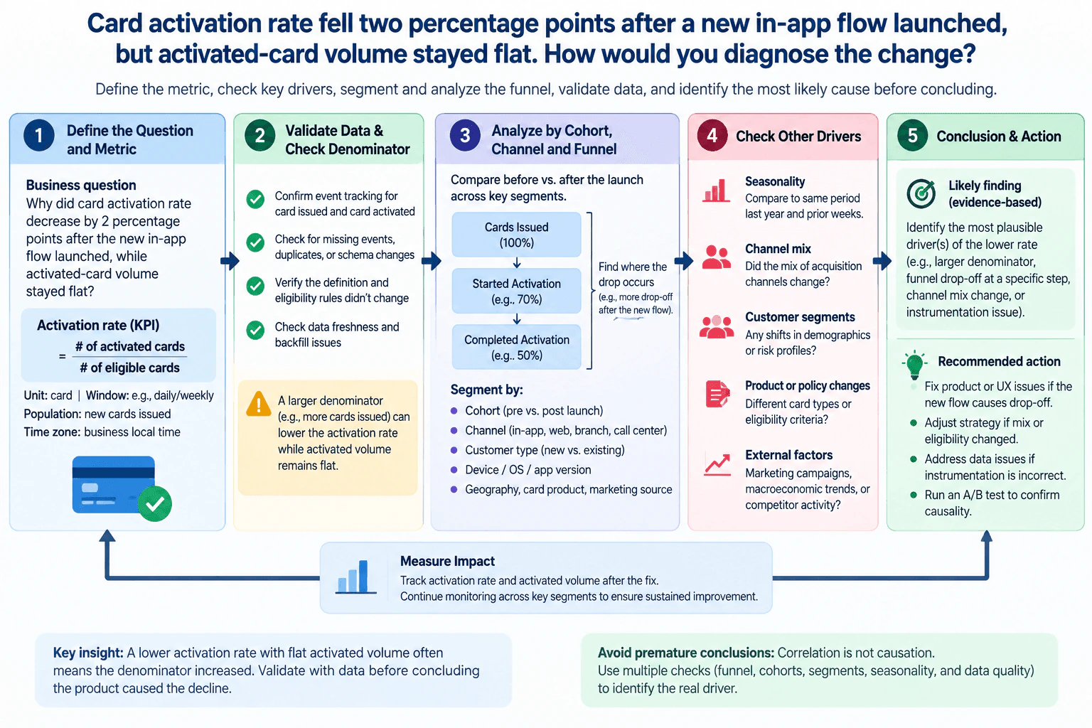
Card activation rate fell two percentage points after a new in-app flow launched, but activated-card volume stayed flat. How would you diagnose the change? diagram
How to Explain It in an Interview

I would structure the analysis from descriptive evidence to diagnosis and then to action.

First, I would define the KPI before interpreting it. Activation rate equals activated cards divided by eligible cards. I would use the card as the unit of analysis and keep the eligible population, reporting window, business reporting time zone, filters, and eligibility rules consistent before and after launch. I would inspect the numerator and denominator separately. Since activated-card volume stayed flat while the rate fell, an increase in eligible cards is mathematically consistent with what we observed. That is a hypothesis to test, not a conclusion.

Second, I would validate the data and instrumentation. I would confirm that events representing card issuance or eligibility and card activation are firing correctly and reconcile application events with the authoritative activation records where available. I would check for missing events, duplicate records, schema or event-name changes, delayed ingestion, backfills, freshness problems, and changes in eligibility logic. I would also compare basic control totals and row counts across the launch boundary. If measurement changed, the apparent KPI decline may be an instrumentation problem rather than a customer-behavior change.

Third, I would analyze the denominator and customer mix. I would compare the eligible-card population before and after launch by card-issue cohort, acquisition or activation channel, customer type, device or operating system, app version, geography, card product, and other relevant segments. This is segmentation analysis: breaking the total population into meaningful groups to see whether the aggregate decline comes from a real within-group change or from a different mix of groups. A larger share of historically lower-activation groups could reduce the overall rate even if each group's own activation rate stayed stable.

Fourth, I would run cohort and funnel analysis. Cohort analysis compares groups formed at a similar point, such as cards issued before versus after the launch, so I can see whether behavior changed for comparable populations. Funnel analysis compares conversion from one required step to the next. Consistent with the diagram, I would examine a flow such as eligible cards, activation flow viewed or started, verification or other required steps, and activation completed. I would compare step conversion before and after launch and break it down by cohort and channel. If the decline is concentrated at one new-flow step while comparable groups remain stable elsewhere, that strengthens the case that the flow is contributing to the problem.

Fifth, I would check other drivers. I would compare matched time windows and examine day-of-week and seasonal patterns. I would look for acquisition-channel shifts, marketing campaigns, customer demographic or risk-profile changes, card-type or eligibility-policy changes, fulfillment or operational changes, macroeconomic conditions, competitor activity, and other concurrent events. I would also check for outliers and sparse segments that could distort the aggregate. These checks matter because a change that happens after a launch is correlated with the launch in time, but correlation alone does not establish causation.

Then I would form the conclusion from the evidence. If the lower rate is explained by denominator growth or a shift toward lower-activation cohorts or channels, I would describe it as a denominator or mix effect rather than a product failure. If the decline remains within comparable cohorts and is concentrated at a specific step introduced by the new flow, I would identify that step as the leading product-related hypothesis. If instrumentation is inconsistent, I would correct the measurement issue before making a product decision.

The recommended action should match the diagnosed driver. If the new flow creates a clear step-level drop-off, I would address that UX or required step. If the denominator or channel mix changed, I would adjust targeting, expectations, or reporting instead of changing the flow unnecessarily. If the data is wrong, I would repair the tracking and recompute the KPI. If causal confidence is important and a controlled experiment is feasible, I would run an A/B test rather than relying only on a before-versus-after comparison.

Finally, I would measure impact. I would track activation rate and activated-card volume together after the action, along with the affected funnel-step conversion rates, by the important cohorts and channels. I would compare them with the same baseline logic used in the diagnosis. If the expected improvement does not appear, I would revisit the hypothesis and continue the feedback loop rather than treating the first explanation as final.

Technical Approach
  1. Define the business decision: determine whether the observed activation-rate decline is caused by the new in-app flow or by another factor.
  2. Define activation rate as activated cards divided by eligible cards, and lock the eligible population, card-level grain, reporting window, business reporting time zone, filters, and baseline.
  3. Reconcile numerator and denominator separately, checking whether the eligible-card denominator increased while activated-card volume stayed flat.
  4. Validate instrumentation, event definitions, eligibility logic, missing or duplicate records, data freshness, delayed ingestion, backfills, and control totals.
  5. Compare pre- and post-launch cohorts and segment the KPI by acquisition or activation channel, customer type, device or OS, app version, geography, card product, and other relevant dimensions.
  6. Analyze the activation funnel step by step: eligible cards, flow viewed or started, verification or required steps, and activation completed; identify where conversion changed.
  7. Check matched time periods, seasonality, day-of-week patterns, marketing campaigns, product or policy changes, customer-segment shifts, macroeconomic or competitive factors, and other concurrent changes.
  8. Separate observed facts from hypotheses and rank the most plausible drivers.
  9. Take an action proportional to the evidence: correct tracking, address a funnel step, or adjust targeting, expectations, or reporting.
  10. If stronger causal evidence is needed and feasible, run a controlled experiment; then monitor activation rate, activated-card volume, and step-level conversion by cohort and channel.
Practical Insights

The main cost is analytical rather than computational. The work requires reconciling eligibility, activation, event, cohort, channel, and segment data and grouping it repeatedly across time and dimensions. More segmentation can reveal the real driver but may create small groups with noisy rates. A simple pre/post comparison is fast but weak for causal conclusions. Cohort and funnel drill-downs take more work but show where the change occurred. A controlled experiment can provide stronger causal evidence, but it requires enough eligible traffic, time, operational support, and appropriate safeguards. The practical tradeoff is speed versus confidence: start with denominator, instrumentation, cohort, channel, and funnel checks, then deepen the analysis where the evidence points.

Why Interviewers Ask This

This tests whether the candidate can distinguish a rate change from a volume change, define the KPI and denominator correctly, validate instrumentation, diagnose denominator and mix effects, use cohort and funnel analysis, consider alternative explanations, and separate correlation from causal evidence before recommending an action.

Common interview mistakes

Common mistakes are blaming the new flow simply because the decline followed the launch; looking only at the activation-rate percentage without reconciling numerator and denominator; comparing different populations, reporting windows, or time zones; ignoring eligibility-rule changes; trusting front-end events without validating instrumentation; analyzing only the aggregate instead of cohorts, channels, and segments; skipping step-level funnel analysis; ignoring seasonality, marketing, product, policy, or external changes; treating a mix shift as a within-segment performance decline; and claiming causation without controlled evidence or sufficiently strong supporting analysis.

Interview tip

Lead with the denominator insight, then give a disciplined sequence: define the KPI, validate data and eligibility, decompose denominator and mix, inspect cohorts and funnel steps, check seasonality and concurrent drivers, and only then discuss causality and action. Explicitly state that flat activated-card volume plus a lower rate is consistent with a larger denominator or mix shift, not proof that the new flow reduced activations.

Interviewer may ask next
What if the overall activation rate fell, but every major cohort's activation rate stayed roughly unchanged?

I would investigate composition before blaming the product. If within-cohort rates are stable but the aggregate falls, the likely explanations are a shift toward cohorts or channels with lower baseline activation rates or a change in the eligible-card denominator. I would calculate each group's share of the eligible population before and after launch and verify that cohort definitions, eligibility logic, time windows, and instrumentation are consistent. I would also look for new or smaller groups omitted from the first breakdown. Unless further evidence shows a within-group decline tied to the new flow, I would describe the result as a denominator or mix effect.

What would you do if the funnel suggests the new flow is hurting activation, but you cannot run an A/B test?

I would strengthen the observational evidence without overstating causality. I would compare matched pre- and post-launch cohorts, use unaffected channels or populations as benchmarks only when they are genuinely comparable, inspect the exact funnel step where conversion changed, and verify that instrumentation and eligibility definitions are stable. I would check seasonality and concurrent business changes and test whether the conclusion holds across reasonable windows and segment definitions. If the same step-level deterioration persists across comparable groups and alternative explanations are weak, I would call the flow the leading hypothesis rather than a proven cause, take a reversible or limited action if justified, and monitor activation rate, activated-card volume, and funnel conversion after the change.

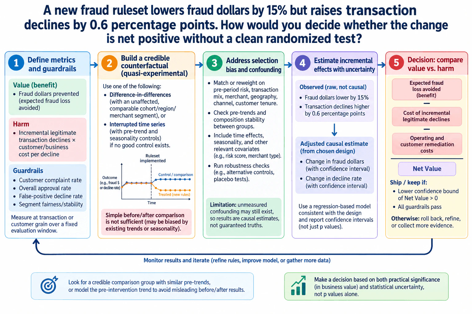
4. A new fraud ruleset lowers fraud dollars by 15% but raises transaction declines by 0.6 percentage points. How would you decide whether the change is net positive without a clean randomized test?Statistics And ExperimentationHardCapital One

Question Details

Define value and harm metrics, identify guardrails, propose a causal or quasi-experimental approach, address selection bias, and state the decision rule.

Short Interview Answer (30-60 seconds)

I would not treat the observed 15% fraud reduction and 0.6 percentage-point increase in declines as causal by themselves. I would define the benefit as expected fraud loss avoided and the harm as incremental legitimate declines multiplied by their customer or business cost, with approval rate, complaints, false-positive declines, and segment fairness as guardrails. Then I would build a counterfactual using difference-in-differences with a comparable unaffected cohort when possible, or interrupted time series if no good control exists. I would adjust for selection bias and confounding, report confidence intervals, and keep the ruleset only if the lower confidence bound of net value is above zero and every guardrail passes.

Detailed Explanation

The task is to decide whether the fraud ruleset creates more business value than harm when there is no clean randomized experiment. The reported 15% drop in fraud dollars and 0.6 percentage-point increase in transaction declines are observed changes, not automatically causal effects. I would first define the value, harm, population, grain, time window, and guardrails. Then I would estimate what would have happened without the ruleset using a credible comparison group or pre-period trend, address selection bias and confounding, quantify uncertainty, and make a conservative decision based on adjusted net value and guardrails.

Useful Questions to Ask the Interviewer
  1. Was the ruleset introduced everywhere at once, or only for certain regions, merchants, channels, customers, or risk segments?
  2. Is there an unaffected cohort with similar pre-change fraud and decline trends that could serve as a comparison group?
  3. How should we value a prevented fraud dollar versus an incremental legitimate decline, including lost revenue, customer friction, and remediation cost?
  4. Which guardrails are mandatory, such as approval rate, customer complaint rate, false-positive decline rate, or segment fairness?
  5. What evaluation window is appropriate, and were there concurrent policy, seasonality, fraud-pattern, pricing, or operational changes?
  6. At what grain should the analysis be performed: transaction, customer, merchant, or another stable unit?
A new fraud ruleset lowers fraud dollars by 15% but raises transaction declines by 0.6 percentage points. How would you decide whether the change is net positive without a clean randomized test? diagram
How to Explain It in an Interview
1. Define the decision, population, grain, and estimands

The decision is whether the new ruleset should be kept, refined, or rolled back. I would define the population exposed to the ruleset, choose a consistent transaction or customer grain, and use a fixed evaluation window so that benefit and harm use compatible denominators and periods.

The main estimands are the incremental change in fraud dollars and the incremental change in legitimate transaction declines attributable to the ruleset relative to the counterfactual outcome that would have occurred without it.

2. Separate observed changes from causal effects

The supplied facts are that fraud dollars are 15% lower and transaction declines are 0.6 percentage points higher. These are raw observed changes. A simple before-and-after comparison is insufficient because fraud patterns, seasonality, transaction mix, customer composition, merchant composition, or other operational changes may have changed at the same time.

So I would treat the 15% and 0.6 percentage-point changes as observations to explain, not proof that the ruleset caused them.

3. Define value, harm, and guardrails

The benefit metric is expected fraud loss avoided. The harm metric is incremental legitimate transaction declines multiplied by the customer or business cost per decline. When defensible business estimates are available, that cost can include lost contribution, customer friction, and remediation effects.

The decision framework is:

Net Value = Expected fraud loss avoided - Cost of incremental legitimate declines - Operating and customer remediation costs.

I would also define guardrails that can block adoption even when estimated net value is positive. Consistent with the diagram, these include customer complaint rate, overall approval rate, false-positive decline rate, and segment fairness or stability.

4. State the hypotheses in decision terms

The null hypothesis is that, after estimating the counterfactual and accounting for uncertainty, the ruleset does not produce positive incremental net value. The alternative hypothesis is that it produces positive incremental net value while all required guardrails remain acceptable.

A p value alone does not answer the business question. Statistical significance concerns whether an estimated effect is distinguishable from sampling variation under the model. Practical significance asks whether the estimated benefit is large enough to outweigh customer harm and operating cost. The decision therefore needs effect sizes, confidence intervals, business value, and guardrails rather than statistical significance alone.

5. Build a credible counterfactual

My preferred approach would be difference-in-differences if I can find an unaffected comparison cohort, region, merchant segment, or other group with similar pre-intervention trends. I would compare how outcomes changed over time in the treated group versus how they changed in the comparison group.

The key identifying assumption is that, without the ruleset, the treated and comparison groups would have followed sufficiently similar outcome trends. I would inspect multiple pre-periods and composition stability rather than relying on a single pre-period value.

If no credible comparison group exists, I would use interrupted time series with enough pre-intervention history to model the existing trend and seasonality, then estimate whether the outcome level or trend changes after implementation. This approach is vulnerable when another event occurs at the same time, so I would state that limitation explicitly.

6. Address selection bias and confounding

Selection bias matters if the ruleset was deployed disproportionately to higher-risk customers, merchants, channels, geographies, or transaction types. A direct exposed-versus-unexposed comparison could then mix pre-existing risk differences with the ruleset effect.

I would match or reweight groups using pre-treatment characteristics such as prior risk, transaction mix, merchant or geography, channel, and customer tenure when those variables are available. I would use a regression model consistent with the chosen design, including relevant time effects, seasonality, and observed covariates that were determined before treatment.

I would then check pre-trends and composition stability and run robustness checks such as alternative comparison groups, placebo intervention dates or outcomes when appropriate, and alternative model specifications. These checks make the result more credible but do not guarantee that unmeasured confounding is absent.

7. Estimate incremental effects with uncertainty

I would estimate the adjusted change in fraud dollars and the adjusted change in decline rate from the chosen quasi-experimental design. For both effects I would report confidence intervals at a pre-specified confidence level rather than reporting only p values.

A confidence interval gives a range of effect values that are reasonably compatible with the observed data and model assumptions. Because this is not a clean randomized experiment, I would also discuss model uncertainty and possible residual bias from unmeasured confounding.

I would propagate the uncertainty in the component estimates into the net-value calculation so that the business decision is based on an uncertainty range for net value, not only a point estimate.

8. Validate the analysis

Before interpreting the result, I would validate transaction or customer grain, exposure timing, row counts, duplicate handling, missing values, outcome definitions, denominators, and consistency across treated and comparison periods. I would check that the evaluation window is long enough to observe the relevant fraud and decline outcomes and that sparse segments are not producing unstable estimates.

I would also check whether the sample provides enough precision for the decision. More data can narrow sampling uncertainty, but additional sample size does not remove confounding in a non-randomized design.

9. Apply the decision rule

I would calculate net value using the adjusted incremental effects rather than directly plugging the raw 15% fraud decrease and 0.6 percentage-point decline increase into the decision.

I would ship or keep the ruleset only if the lower confidence bound of Net Value is above zero and every required guardrail passes. This matches the diagram's conservative rule: the estimated benefit must remain positive even at the lower end of the uncertainty interval, and customer-harm constraints must still be satisfied.

If net value is negative, a guardrail fails, or the result is highly sensitive to reasonable design or modeling choices, I would roll back or refine the ruleset. If the evidence remains inconclusive, I would collect more evidence or create a stronger targeted holdout or controlled rollout when operationally possible.

10. State the limitation and monitoring loop

The main limitation is unmeasured confounding. Matching, reweighting, regression controls, fixed effects, pre-trend checks, and placebo tests can reduce or reveal some biases, but they cannot prove that every important confounder has been measured.

After a decision, I would keep monitoring fraud loss, decline rate, approval rate, customer complaints, false-positive declines, and segment-level stability. If fraud patterns, transaction mix, model behavior, or guardrails drift, I would refine the rules, improve the model, or gather more data and repeat the evaluation.

Technical Approach
  1. Define the exposed population, analysis grain, evaluation window, fraud outcome, legitimate-decline outcome, business-value inputs, and guardrails.
  2. Treat the observed 15% fraud decrease and 0.6 percentage-point decline increase as raw associations rather than causal effects.
  3. Define Net Value as expected fraud loss avoided minus the cost of incremental legitimate declines minus operating and customer-remediation costs.
  4. Use difference-in-differences with a comparable unaffected cohort when credible; otherwise use interrupted time series with pre-trend and seasonality controls if appropriate.
  5. Check pre-trends, composition stability, exposure timing, and data quality.
  6. Match or reweight on pre-treatment characteristics and use regression consistent with the chosen design to address observed selection bias and confounding.
  7. Run robustness checks such as alternative controls, placebo tests, and alternative specifications.
  8. Estimate adjusted fraud and decline effects with confidence intervals and propagate uncertainty into net value.
  9. Ship or keep the ruleset only if the lower confidence bound of net value is above zero and all guardrails pass; otherwise roll back, refine, or gather stronger evidence.
  10. Monitor results and repeat the analysis if conditions change.
Practical Insights

The main cost is analytical rather than computational. You need enough historical data to establish pre-trends, a credible comparison group or stable time series, consistent transaction or customer-level data, and defensible business inputs for valuing fraud and legitimate declines. Matching, weighting, regression controls, confidence intervals, placebo tests, and sensitivity checks require more analysis effort but reduce the chance of making a decision from a misleading before-and-after comparison. The largest remaining limitation is that a sophisticated observational model can adjust for measured differences but cannot eliminate bias from important unmeasured confounders.

Why Interviewers Ask This

This tests whether the candidate can separate an observed before-and-after change from a credible causal estimate, translate fraud reduction and customer friction into comparable business value, identify selection bias and confounding, quantify uncertainty, enforce guardrails, and make a decision no stronger than the evidence supports.

Common interview mistakes

Common mistakes are treating the observed 15% fraud reduction as caused by the ruleset without a credible counterfactual; treating the 0.6 percentage-point decline increase as automatically unacceptable without valuing the benefit; relying on a simple before-and-after comparison despite seasonality or existing trends; choosing a comparison group with different pre-trends; ignoring selection bias from how the ruleset was deployed; controlling for variables affected by treatment instead of pre-treatment confounders; reporting only p values instead of effect sizes and confidence intervals; ignoring false-positive declines, approval rate, complaints, or segment fairness; mixing incompatible denominators or time windows; claiming that matching or regression eliminates all confounding; and approving the ruleset because the point estimate of net value is positive even when the lower confidence bound is not above zero or a guardrail fails.

Interview tip

Present the answer in this order: observed facts, value and harm metrics, guardrails, counterfactual design, selection-bias checks, uncertainty, and decision rule. Explicitly say that the 15% and 0.6 percentage-point changes are raw observations until a credible quasi-experimental design supports a causal interpretation. Finish with the rule shown in the diagram: ship only when the lower confidence bound of net value is above zero and every guardrail passes.

Interviewer may ask next
What would you do if the treated and comparison groups have clearly different pre-intervention trends?

I would not trust a basic difference-in-differences estimate because the comparison group would not provide a credible counterfactual. I would look for a better comparison cohort, refine matching or weighting using pre-treatment characteristics, or use another defensible design such as interrupted time series if there is enough stable pre-period history. I would run placebo and sensitivity checks and weaken the causal claim if the identifying assumptions remain doubtful. If no design produces credible evidence, I would recommend collecting stronger evidence, ideally through a targeted holdout or staged controlled rollout.

What if the estimated net value is positive but its confidence interval includes zero?

I would treat the result as inconclusive rather than call the ruleset net positive. The point estimate suggests potential value, but the uncertainty range still includes no benefit or a loss. Under the diagram's decision rule, I would not ship solely on that point estimate because the lower confidence bound is not above zero. I would identify which component drives the uncertainty, check model sensitivity and guardrails, collect more data if useful, or refine the ruleset. If the business must act before uncertainty is resolved, I would describe that as a risk-managed business decision rather than a statistically supported net-positive conclusion.

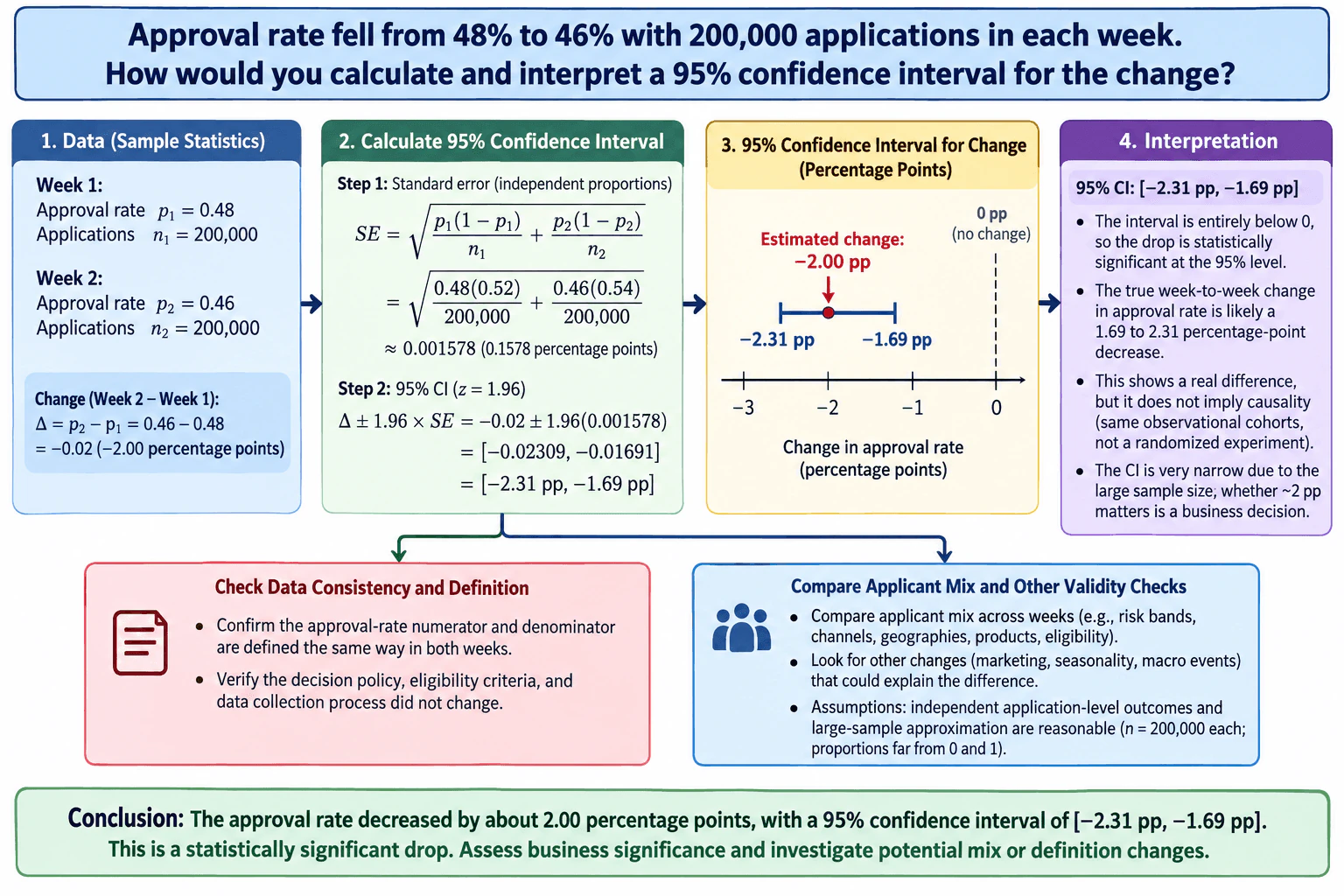
5. Approval rate fell from 48% to 46% with 200,000 applications in each week. How would you calculate and interpret a 95% confidence interval for the change?Statistics And ExperimentationMediumCapital One

Question Details

State the formula or method, assumptions, interpretation, practical significance, and checks for definition or applicant-mix changes.

Short Interview Answer (30-60 seconds)

I would define the change as Week 2 minus Week 1, so the estimate is 46% - 48% = -2.00 percentage points. Assuming independent weekly samples, the standard error is sqrt[0.48(0.52)/200,000 + 0.46(0.54)/200,000] ≈ 0.001578. The 95% confidence interval is -0.02 ± 1.96 × 0.001578, which is about [-2.31, -1.69] percentage points. Since zero is not in the interval, the decline is statistically significant. I would separately assess whether a roughly two-point drop matters to the business and verify that the approval definition and applicant mix did not change.

Detailed Explanation

The task is to estimate how much the approval rate changed from one week to the next and quantify the uncertainty around that estimate. Week 1 has a sample approval rate of 48% from 200,000 applications, and Week 2 has 46% from 200,000 applications. The observed change is therefore -2.00 percentage points. I would use a confidence interval for the difference between two proportions, assuming the weekly application outcomes are sufficiently independent. Then I would interpret the interval, separate statistical significance from business importance, and check whether definitions or applicant composition changed.

Useful Questions to Ask the Interviewer
  1. Are the two weeks made up of different applicants, or can the same applicant appear in both weeks?
  2. Was an approval defined exactly the same way in both weeks, with the same numerator and denominator rules?
  3. Did eligibility criteria, decision policy, data collection, or application processing change between the weeks?
  4. Did the applicant mix change by important characteristics such as risk band, geography, product, or acquisition channel?
  5. Is there a business threshold for what size approval-rate change would be considered practically important?
Approval rate fell from 48% to 46% with 200,000 applications in each week. How would you calculate and interpret a 95% confidence interval for the change? diagram
How to Explain It in an Interview

First, define the estimand clearly. Let p1 represent the underlying Week 1 approval probability and p2 the underlying Week 2 approval probability. The sample estimates are p̂1 = 0.48 and p̂2 = 0.46. Define the change as Δ = p2 - p1, so the sample estimate is Δ̂ = 0.46 - 0.48 = -0.02, which is a decrease of 2.00 percentage points.

For a two-sided significance framing, the null hypothesis is H0: Δ = 0, meaning no difference in the underlying approval rates, and the alternative hypothesis is H1: Δ ≠ 0. The confidence interval addresses the same comparison while also showing the plausible magnitude of the difference.

Assuming the two weekly samples can be treated as independent, the standard error for the difference in sample proportions is:

SE(Δ̂) = sqrt[p̂1(1-p̂1)/n1 + p̂2(1-p̂2)/n2].

Substituting the supplied values:

SE = sqrt[0.48(0.52)/200,000 + 0.46(0.54)/200,000] ≈ 0.001578.

That is about 0.1578 percentage points. For a 95% confidence interval, use the large-sample critical value 1.96:

Δ̂ ± 1.96 × SE = -0.02 ± 1.96(0.001578) ≈ -0.02 ± 0.00309 = [-0.02309, -0.01691].

Expressed in percentage points, the 95% confidence interval is approximately [-2.31, -1.69] percentage points. The point estimate is -2.00 percentage points, which lies at the center of that interval.

Because the entire interval is below zero, the observed decrease is statistically significant at the 5% two-sided level under the stated assumptions. A careful frequentist interpretation is that if we repeatedly sampled in the same way and constructed intervals using this procedure, about 95% of those intervals would contain the true Week 2 minus Week 1 difference. I would not say there is a 95% probability that this one fixed population difference lies inside this particular interval.

The interval is narrow largely because each week contains 200,000 applications. Statistical significance, however, is not the same as practical significance. Whether a decrease of roughly two percentage points matters depends on business impact, risk objectives, customer impact, and any predefined materiality threshold. Those inputs are not supplied, so I would not invent a business conclusion.

I would also avoid a causal claim. The question describes two weekly cohorts, not a randomized experiment. A statistically significant difference shows a measurable week-to-week association under the model assumptions, but it does not prove that a particular policy, product change, or other intervention caused the decline.

The most important validity checks are definition consistency and applicant-mix consistency. I would confirm that the approval-rate numerator and denominator were defined the same way in both weeks and that eligibility criteria, decision policy, and data collection were unchanged. I would compare applicant distributions across relevant segments such as risk bands, channels, geographies, or products if those fields are available. A change in applicant composition can move the aggregate approval rate even when within-segment approval behavior is stable.

The calculation also assumes application-level outcomes are sufficiently independent and that the large-sample normal approximation is reasonable. With n = 200,000 in each week and approval proportions far from 0 and 1, the normal approximation is appropriate. If the same applicants can appear repeatedly, observations are clustered, or the weeks are otherwise dependent, I would use a method that accounts for that dependence rather than the simple independent-samples formula.

If applicant-mix differences are material, I would not treat the raw two-proportion interval as the whole story. I could stratify the comparison using comparable segments or fit an appropriate regression model to estimate an adjusted week association while controlling for measured applicant characteristics. That can address observed composition differences, but it still does not turn an observational comparison into a randomized causal estimate.

Finally, I would validate the result by reproducing the numerator, denominator, and sample counts for both weeks, checking for duplicate or repeated applications when relevant, confirming the metric definition, and independently recalculating the interval. My conclusion would be: the observed approval rate fell by 2.00 percentage points, with a 95% confidence interval of approximately -2.31 to -1.69 percentage points. That is statistically significant under the stated assumptions, while practical significance and the reason for the decline require separate investigation.

Technical Approach

1. Define the direction of change as Week 2 minus Week 1. 2. Record p̂1 = 0.48, p̂2 = 0.46, and n1 = n2 = 200,000. 3. Calculate Δ̂ = p̂2 - p̂1 = -0.02. 4. Assuming independent weekly samples, calculate SE = sqrt[p̂1(1-p̂1)/n1 + p̂2(1-p̂2)/n2] ≈ 0.001578. 5. Construct the 95% interval as Δ̂ ± 1.96 × SE, giving approximately [-0.02309, -0.01691], or [-2.31, -1.69] percentage points. 6. Check whether zero is inside the interval to assess two-sided statistical significance. 7. Separately evaluate practical significance. 8. Validate the approval definition, denominator, policy, data collection process, independence assumption, and applicant mix before drawing an operational conclusion.

Practical Insights

Once the two weekly approval rates and sample sizes are known, the confidence-interval calculation itself is constant work because it needs only a few arithmetic operations. The more important cost is validation. If raw application-level data must be checked for duplicates, repeated applicants, definition consistency, or segment mix, that work generally grows with the number of application records. With only the supplied aggregate rates and sample sizes, the calculation is fast but cannot by itself detect data-quality or composition changes.

Why Interviewers Ask This

This tests whether the candidate can calculate uncertainty for a difference in proportions, interpret a confidence interval correctly, distinguish statistical significance from practical significance, and recognize that a week-over-week comparison can be distorted by definition changes, applicant-mix shifts, selection bias, or other confounding factors.

Common interview mistakes

Common mistakes are subtracting in the wrong direction and then interpreting the sign incorrectly; reporting a 2% relative decline when the observed difference is 2 percentage points; using only one proportion's variance instead of both; treating the confidence interval as a 95% probability statement about the fixed true parameter; claiming causality from a non-randomized week-over-week comparison; assuming statistical significance automatically means business importance; ignoring repeated applicants or dependence between weeks; and failing to check whether the approval definition, eligibility rules, decision policy, denominator, or applicant mix changed.

Interview tip

State the direction first: 'Week 2 minus Week 1.' Then give the estimate, standard-error formula, and interval in percentage points. Say clearly that the interval is entirely below zero, so the decrease is statistically significant under the independence and large-sample assumptions. Finish by separating business significance from statistical significance and naming the two most important validity checks: consistent approval definitions and comparable applicant mix.

Interviewer may ask next
What would you do if some applicants appeared in both weeks, so the two samples were not independent?

I would not use the simple independent-proportions standard error without adjustment because repeated applicants create dependence. I would identify applicants across weeks and choose a method that matches the data structure. If outcomes are naturally paired for the same units, I would use a paired method based on the joint outcomes. If applicants can contribute multiple correlated observations, I could use an appropriate regression model with cluster-robust standard errors at the applicant level or another repeated-measures method. I would first quantify how much overlap exists because the uncertainty estimate must reflect the actual dependence structure.

What if the overall approval rate fell by two percentage points, but the applicant mix changed substantially between the two weeks?

The raw confidence interval would still describe the difference between the two observed weekly aggregate rates, but it might not represent a like-for-like change. I would compare the applicant distributions across relevant segments, calculate within-segment approval rates, and determine whether composition shifts explain part of the aggregate decline. If appropriate fields are available, I could standardize the mix or use a regression model to estimate an adjusted week association while controlling for measured characteristics. I would report the unadjusted and adjusted views when useful, and I would still avoid a causal interpretation unless the study design supports one.

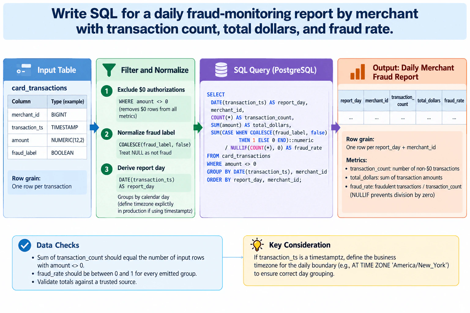
6. Write SQL for a daily fraud-monitoring report by merchant with transaction count, total dollars, and fraud rate.Sql And DatabasesEasyCapital One

Question Details

Use card_transactions(merchant_id, transaction_ts, amount, fraud_label). Exclude $0 authorizations, treat a null fraud label as not fraud, and prevent division by zero.

Short Interview Answer (30-60 seconds)

I would filter out amount = 0 rows first, derive the reporting day from transaction_ts, and group by that day and merchant_id. COUNT() gives the transaction count, SUM(amount) gives total dollars, and a CASE expression converts fraud_label into 1 for fraud and 0 otherwise, with COALESCE treating NULL as not fraud. I would cast the fraud count to numeric and divide by NULLIF(COUNT(), 0) so the rate uses decimal division and cannot divide by zero. I would also confirm the business timezone before defining a day.

Detailed Explanation

See the Code while reading this explanation.

The goal is to produce one daily report row for each merchant from card_transactions. Each input row represents one transaction. First, remove $0 authorizations because they should not count in any metric. Then convert transaction_ts to a reporting day and group by that day plus merchant_id. Count the remaining transactions, sum their amount, and count fraud by treating only true fraud_label values as fraud while treating NULL as not fraud. Finally, divide fraud count by transaction count using numeric division and NULLIF for defensive zero-denominator handling. The result grain is one row per report_day and merchant_id.

Useful Questions to Ask the Interviewer
  1. What timezone defines the reporting day if transaction_ts includes timezone information?
  2. Is amount guaranteed to use one currency, or should currencies be separated before summing dollars?
  3. Can the source contain duplicate transaction rows that must be removed before aggregation?
Write SQL for a daily fraud-monitoring report by merchant with transaction count, total dollars, and fraud rate. diagram
How to Explain It in an Interview

Start with the grain. The input grain is one row per transaction. The required output grain is one row per report_day plus merchant_id. There is only one source table, so no JOIN is required and there is no join-related row multiplication to manage.

The first rule is to exclude $0 authorizations. Applying WHERE amount <> 0 before aggregation means those rows are excluded consistently from transaction_count, total_dollars, and the fraud-rate denominator.

Next, derive the reporting day with DATE(transaction_ts). That creates the daily grouping key shown in the diagram. If transaction_ts is a timestamptz, I would first confirm the business timezone because converting a timestamp to a date under the wrong timezone can place a transaction on the wrong reporting day.

Then GROUP BY DATE(transaction_ts), merchant_id. COUNT() counts the remaining non-$0 transactions. SUM(amount) gives the total dollars for that merchant and day.

For fraud, use CASE WHEN COALESCE(fraud_label, false) THEN 1 ELSE 0 END. COALESCE makes the required null rule explicit: a NULL fraud_label is treated as not fraud. Summing this CASE expression produces the number of fraudulent transactions in the group.

Fraud rate is fraudulent transactions divided by transaction count. Cast the fraud-count sum to numeric so PostgreSQL performs decimal division rather than integer division. Use NULLIF(COUNT(), 0) as the denominator so a zero count would produce NULL rather than a division-by-zero error. With this grouped query, every emitted group has at least one post-filter row, so the denominator is positive for emitted groups; NULLIF remains a defensive safeguard.

ORDER BY report_day, merchant_id makes the returned report deterministic and easy to inspect. It does not change the calculations. The output columns are report_day, merchant_id, transaction_count, total_dollars, and fraud_rate.

For validation, I would check that the sum of transaction_count across all output groups equals the number of source rows where amount <> 0. I would check that every emitted fraud_rate is between 0 and 1, and I would compare report totals with a trusted control source. I would also verify the reporting timezone and investigate duplicate source rows if the table does not guarantee transaction-level uniqueness.

Technical Approach

1. Confirm the reporting timezone and that the source grain is one transaction per row. 2. Filter card_transactions to amount <> 0. 3. Derive report_day from transaction_ts. 4. Group by report_day and merchant_id. 5. Calculate COUNT() as transaction_count. 6. Calculate SUM(amount) as total_dollars. 7. Convert fraud_label to a 1/0 indicator with CASE and COALESCE, then sum it. 8. Cast the fraud count to numeric and divide by NULLIF(COUNT(), 0) for fraud_rate. 9. Order by report_day and merchant_id. 10. Validate row counts, fraud-rate bounds, totals, duplicates, and date boundaries.

Practical Complexity & Trade-offs

The query scans the qualifying transaction rows and groups them by day and merchant. Conceptually, the work grows with the number of transactions being reported. GROUP BY needs memory or temporary storage for the merchant-day groups, and ORDER BY can add sorting work. For a large table, restricting the query to the required reporting period would usually reduce the amount of data processed. Specific index or partition recommendations depend on the actual workload and table design, which are not provided.

Example

PostgreSQL implementation matching the diagram. It excludes zero-dollar authorizations before aggregation, treats NULL fraud labels as false, preserves one row per report day and merchant, uses numeric division for the fraud rate, and protects the denominator with NULLIF.

Code
SELECT
  DATE(transaction_ts) AS report_day,
  merchant_id,
  COUNT(*) AS transaction_count,
  SUM(amount) AS total_dollars,
  CAST(
    SUM(
      CASE
        WHEN COALESCE(fraud_label, FALSE) THEN 1
        ELSE 0
      END
    ) AS NUMERIC
  ) / NULLIF(COUNT(*), 0) AS fraud_rate
FROM
  card_transactions
WHERE
  amount <> 0
GROUP BY
  DATE(transaction_ts),
  merchant_id
ORDER BY
  report_day,
  merchant_id;
Where it is used

This pattern is useful for daily fraud monitoring, merchant risk reporting, operational dashboards, reconciliation reports, and other analyst reports that aggregate transaction-level data into one row per business entity and day.

Why Interviewers Ask This

This tests whether you can translate reporting rules into correct SQL while preserving the required data grain, filters, null behavior, aggregation, denominator logic, and date boundaries. The interviewer wants to see that you can produce one reliable daily row per merchant and validate the result instead of only writing syntactically valid SQL.

Common interview mistakes

Including amount = 0 authorizations in the metrics; using COUNT(fraud_label), which counts both true and false non-NULL labels rather than fraudulent rows; allowing NULL fraud labels to propagate instead of treating them as not fraud; using integer division for fraud_rate; forgetting defensive zero-denominator handling; grouping by merchant without the reporting day; assuming DATE(transaction_ts) uses the intended business timezone; or adding joins that multiply transaction rows unnecessarily.

Interview tip

State the input and output grain before writing SQL. Then explain the query in the same order as the diagram: filter, normalize NULL fraud labels, derive the day, aggregate, calculate the rate, and validate the totals. Mention the timezone boundary because it shows you are thinking about production reporting, not only syntax.

Interviewer may ask next
What would you change if transaction_ts is a timestamptz and the business day must follow a specific local timezone?

I would convert transaction_ts to the agreed business timezone before deriving the date, then group by that timezone-adjusted date. The exact expression depends on how the timestamp is stored and the chosen timezone. I would use the same expression consistently in SELECT and GROUP BY and test transactions around midnight and daylight-saving transitions to confirm the reporting boundary.

What would you do if duplicate transaction rows are possible in card_transactions?

I would first identify the transaction's true unique key or documented deduplication rule. Then I would deduplicate at the transaction grain before the GROUP BY, for example in a CTE using that key and an appropriate deterministic rule. I would not invent a key from merchant_id, transaction_ts, amount, and fraud_label because different legitimate transactions can share those values. After deduplication, I would rerun the same merchant-day aggregation and compare counts and totals with a trusted control source.

7. Write SQL to calculate seven-day credit-card account conversion by acquisition channel.Sql And DatabasesHardCapital One

Question Details

Cohort customers by their first campaign exposure, deduplicate repeated exposures, count an account opened within seven days, and exclude customers who already had a card account before exposure.

Short Interview Answer (30-60 seconds)

I would first reduce campaign_exposures to one row per customer using ROW_NUMBER() ordered by exposure_ts and exposure_id. Then I would exclude anyone with a card_accounts row opened before that first exposure. For each remaining customer, I would use EXISTS to flag whether at least one account opened in the half-open window from first_exposure_ts through, but not including, first_exposure_ts + 7 days. Finally, I would GROUP BY acquisition_channel and calculate eligible customers, converted customers, and conversion rate.

Detailed Explanation

See the Code while reading this explanation.

The goal is to measure what share of newly eligible customers open a credit-card account within seven days of their first campaign exposure, grouped by the channel of that first exposure. The key is to keep exactly one cohort row per customer before looking at accounts. Repeated exposures must not increase the denominator, and multiple account rows must not increase the numerator. Customers who already had a card account before exposure are removed. The seven-day window is handled as [first exposure, first exposure + 7 days), then the customer-level flags are aggregated by channel.

Useful Questions to Ask the Interviewer
  1. Are exposure_ts and opened_ts stored in the same time zone and comparable timestamp type?
  2. Does card_accounts contain only credit-card accounts, or is a product filter required?
  3. Should an account opened exactly seven days after exposure count? I would use a half-open window, so it would not.
  4. Can channel be NULL, and should NULL be reported as its own group or excluded?
  5. If two exposures have the same exposure_ts, is exposure_id the accepted deterministic tie-breaker?
Write SQL to calculate seven-day credit-card account conversion by acquisition channel. diagram
How to Explain It in an Interview

Start with grain. campaign_exposures has one row per exposure, so a customer can appear many times. card_accounts has one row per account, so a customer can also appear many times there. The required cohort grain is one row per customer, and the final result grain is one row per acquisition channel.

First, rank campaign exposures within each customer using ROW_NUMBER(). Ordering by exposure_ts and then exposure_id makes the first exposure deterministic when timestamps tie. Keep only rn = 1, retain the corresponding acquisition_channel, and rename exposure_ts to first_exposure_ts. This creates the first_exposure CTE with exactly one row per customer.

Second, create eligible_customers by removing anyone who already had a card account before first_exposure_ts. NOT EXISTS is appropriate because this is a yes-or-no eligibility test. It avoids joining every prior account row to the customer and therefore prevents row multiplication from the one-to-many relationship between customers and card accounts.

Third, create customer_conversion and keep one row per eligible customer. Use EXISTS to check whether at least one card_accounts row satisfies opened_ts >= first_exposure_ts and opened_ts < first_exposure_ts + INTERVAL '7 days'. This is the half-open interval [first exposure, first exposure + 7 days). An account opened exactly at first exposure counts; an account opened exactly seven days later does not. EXISTS returns one Boolean result regardless of how many qualifying accounts exist, so each customer contributes at most one conversion. A CASE expression turns that result into converted_flag = 1 or 0.

Finally, GROUP BY acquisition_channel. COUNT() is the eligible-customer denominator because customer_conversion remains one row per eligible customer. SUM(converted_flag) is the converted-customer numerator. The conversion rate is 1.0 * SUM(converted_flag) / COUNT(). The output grain is one row per acquisition channel.

Before trusting the result, validate the grain at each stage. first_exposure should have at most one row per customer. eligible_customers should contain no customer with a card account opened before first_exposure_ts. customer_conversion should still contain exactly one row per eligible customer. Check for unexpected NULL values in customer_id, exposure_ts, opened_ts, or channel because NULL comparisons can evaluate to unknown and change eligibility or conversion behavior. Confirm that both timestamps use compatible time-zone semantics. Reconcile eligible and converted totals against a trusted source or an independently computed control total. If card_accounts includes products other than credit cards, apply the same credit-card product filter consistently in both the prior-account exclusion and conversion checks.

Technical Approach

1. Define the source grain: campaign_exposures is one row per exposure and card_accounts is one row per account. 2. Rank each customer's exposures with ROW_NUMBER() ordered by exposure_ts, exposure_id. 3. Keep rn = 1 to produce one first-exposure row per customer and retain that row's acquisition channel. 4. Exclude customers for whom a card_accounts row exists with opened_ts < first_exposure_ts. 5. For each eligible customer, set converted_flag = 1 when any account exists with opened_ts >= first_exposure_ts and opened_ts < first_exposure_ts + INTERVAL '7 days'; otherwise set it to 0. 6. GROUP BY acquisition_channel and compute eligible customers, converted customers, and conversion rate. 7. Validate row uniqueness, exclusion logic, NULL handling, timestamp boundaries, and control totals.

Practical Complexity & Trade-offs

The main costs are ranking exposure rows and searching account rows by customer and time. ROW_NUMBER() can require sorting exposures within each customer. The two EXISTS checks are useful because they test whether a qualifying account exists without returning every matching account row. On large tables, performance depends on the actual query plan and available indexes, especially access paths involving customer_id and timestamps. Index recommendations should be confirmed with the real schema and EXPLAIN plan rather than assumed.

Example

PostgreSQL implementation matching the approved diagram: rank and deduplicate first exposure, exclude pre-existing cardholders with NOT EXISTS, flag seven-day conversion with EXISTS, and aggregate by acquisition channel. The query preserves one row per customer before the final GROUP BY, so repeated exposures and multiple matching account rows cannot inflate the denominator or numerator.

Code
WITH
  ranked_exposures AS (
    SELECT
      customer_id,
      channel AS acquisition_channel,
      exposure_ts,
      exposure_id,
      ROW_NUMBER() OVER (
        PARTITION BY
          customer_id
        ORDER BY
          exposure_ts,
          exposure_id
      ) AS rn
    FROM
      campaign_exposures
  ),
  first_exposure AS (
    SELECT
      customer_id,
      acquisition_channel,
      exposure_ts AS first_exposure_ts
    FROM
      ranked_exposures
    WHERE
      rn = 1
  ),
  eligible_customers AS (
    SELECT
      fe.customer_id,
      fe.acquisition_channel,
      fe.first_exposure_ts
    FROM
      first_exposure fe
    WHERE
      NOT EXISTS (
        SELECT
          1
        FROM
          card_accounts ca
        WHERE
          ca.customer_id = fe.customer_id
          AND ca.opened_ts < fe.first_exposure_ts
      )
  ),
  customer_conversion AS (
    SELECT
      e.customer_id,
      e.acquisition_channel,
      e.first_exposure_ts,
      CASE
        WHEN EXISTS (
          SELECT
            1
          FROM
            card_accounts ca
          WHERE
            ca.customer_id = e.customer_id
            AND ca.opened_ts >= e.first_exposure_ts
            AND ca.opened_ts < e.first_exposure_ts + INTERVAL '7 days'
        ) THEN 1
        ELSE 0
      END AS converted_flag
    FROM
      eligible_customers e
  )
SELECT
  acquisition_channel,
  COUNT() AS eligible_customers,
  SUM(converted_flag) AS converted_customers,
  1.0 * SUM(converted_flag) / COUNT() AS conversion_rate
FROM
  customer_conversion
GROUP BY
  acquisition_channel
ORDER BY
  acquisition_channel;
Where it is used

This pattern is useful for campaign attribution, acquisition-channel reporting, onboarding funnels, trial-to-paid conversion, and other analyses where each person must be assigned to a first event, prior participants must be excluded, and conversion is measured within a fixed post-event window.

Why Interviewers Ask This

This tests whether the candidate can define the correct cohort and row grain, use a window function to select each customer's first campaign exposure, exclude pre-existing cardholders without multiplying rows, apply an exact seven-day timestamp boundary, and aggregate a trustworthy conversion rate by acquisition channel.

Common interview mistakes

Common mistakes are counting every campaign exposure instead of only the first, using a non-deterministic tie when exposure timestamps match, directly joining one-to-many account rows and multiplying customers, excluding customers based on accounts opened after exposure, using an inconsistent seven-day boundary, ignoring NULL timestamp behavior, filtering credit-card products in only one of the two account checks, or aggregating before restoring one row per customer.

Interview tip

State the row grain before writing SQL: one row per exposure, one row per account, then one row per customer before the final aggregation. That makes the ROW_NUMBER(), NOT EXISTS, EXISTS, CASE, and GROUP BY choices easy to justify.

Interviewer may ask next
What would you change if an account opened exactly seven days after the first exposure should count as a conversion?

I would change only the upper-bound predicate from ca.opened_ts < e.first_exposure_ts + INTERVAL '7 days' to ca.opened_ts <= e.first_exposure_ts + INTERVAL '7 days'. I would also confirm that exposure_ts and opened_ts use compatible timestamp types, precision, and time-zone semantics so the inclusive boundary is interpreted consistently.

What if card_accounts contains checking, savings, and credit-card accounts instead of only credit-card accounts?

I would add the same explicit credit-card product predicate inside both account checks: the NOT EXISTS block that excludes pre-existing cardholders and the EXISTS block that flags seven-day conversion. Applying the product filter in only one place would create an inconsistent cohort, so the credit-card definition must be identical for eligibility and conversion.

8. Write SQL to return every neighborhood that currently has zero users.Sql And DatabasesEasyCapital One

Question Details

Assume neighborhoods(neighborhood_id, neighborhood_name) and users(user_id, neighborhood_id). Preserve neighborhoods with no matching users and explain how nulls affect the query.

Short Interview Answer (30-60 seconds)

I would start from neighborhoods because every neighborhood row must remain eligible for the result. Then I would LEFT JOIN users on neighborhood_id and filter with u.neighborhood_id IS NULL. A LEFT JOIN keeps an unmatched neighborhood and fills the users-side columns with NULL, so that NULL test identifies neighborhoods with no matching user row. I would test the joined neighborhood_id rather than assume user_id is non-null, because the supplied schema does not declare key constraints.

Detailed Explanation

See the Code while reading this explanation.

The task is to return neighborhood rows for which no user row matches the same neighborhood_id. Start from neighborhoods because those are the rows that must be preserved. A LEFT JOIN keeps every left-side neighborhood row even when no users row matches it. For an unmatched neighborhood, the columns contributed by users are NULL. Filtering on u.neighborhood_id IS NULL therefore keeps only those unmatched rows. The output grain is neighborhood rows from neighborhoods that have no matching users. No sample values, primary keys, foreign keys, uniqueness rules, or active-status fields are supplied, so they should not be assumed.

Useful Questions to Ask the Interviewer
  1. Should duplicate rows in neighborhoods be returned as stored, or should the output represent unique neighborhoods?
  2. Is neighborhood_id the intended relationship between the two tables, as shown in the supplied schema?
  3. Does "currently" simply mean the present contents of users, or is there an active-status or date field that is not shown?
Write SQL to return every neighborhood that currently has zero users. diagram
How to Explain It in an Interview

First explain the join grain. neighborhoods provides the rows we need to preserve. users may contain multiple rows with the same neighborhood_id, so a matching neighborhood can produce multiple joined rows before filtering. Those matched rows have a non-NULL u.neighborhood_id and are removed by the WHERE clause. A neighborhood with no matching users produces one LEFT JOIN row whose users-side columns are NULL.

The query is:

SELECT n.neighborhood_id,
       n.neighborhood_name
FROM neighborhoods AS n
LEFT JOIN users AS u
    ON n.neighborhood_id = u.neighborhood_id
WHERE u.neighborhood_id IS NULL;

The ON condition matches rows only when n.neighborhood_id = u.neighborhood_id evaluates to true. If no users row matches, LEFT JOIN still keeps the neighborhood and supplies NULL for the users-side fields. The WHERE clause then keeps exactly those rows where the joined users.neighborhood_id is NULL.

NULL handling matters because SQL uses three-valued logic. A comparison such as column = NULL does not evaluate to true; use IS NULL to test for NULL. Testing u.neighborhood_id is robust for this anti-join because it is the column used in the equality join: any row that actually satisfies n.neighborhood_id = u.neighborhood_id must have a non-NULL u.neighborhood_id for that matched row. If n.neighborhood_id itself is NULL, it cannot equality-match a users row, so that neighborhood row is treated as having no matching user under this join condition.

An INNER JOIN would be wrong because it removes neighborhoods with no matches, which are exactly the rows requested. GROUP BY and HAVING could solve the problem, but they add unnecessary aggregation for this direct anti-join. NOT EXISTS is another valid formulation, but LEFT JOIN plus IS NULL matches the diagram's requested preservation flow directly.

For validation, verify that every returned neighborhood row has no users row satisfying users.neighborhood_id = neighborhoods.neighborhood_id. Also check whether neighborhoods contains duplicates if the business expects one unique output row per real-world neighborhood, because the supplied schema does not declare a uniqueness constraint.

Technical Approach
  1. Start from neighborhoods so all neighborhood rows remain eligible for the result.
  2. LEFT JOIN users on n.neighborhood_id = u.neighborhood_id.
  3. Keep rows where u.neighborhood_id IS NULL.
  4. Select n.neighborhood_id and n.neighborhood_name.
  5. Validate that each returned row has no matching users.neighborhood_id and clarify duplicate-neighborhood expectations if uniqueness matters.
Practical Complexity & Trade-offs

The SQL is simple, but physical cost depends on the database engine, table sizes, available indexes, and execution plan, none of which are supplied. Conceptually, the database must determine whether each neighborhood has a matching users row. An index on users.neighborhood_id may help some engines, but it is not required for correctness and should not be claimed as present. The LEFT JOIN form is easy to read and does not require GROUP BY, HAVING, or DISTINCT for the stated logic.

Example

Use neighborhoods as the preserved left side, LEFT JOIN users on neighborhood_id, then filter on the joined users.neighborhood_id being NULL. This follows the diagram directly and does not assume that user_id is a primary key or non-null column.

Code
SELECT
  n.neighborhood_id,
  n.neighborhood_name
FROM
  neighborhoods AS n
  LEFT JOIN users AS u ON n.neighborhood_id = u.neighborhood_id
WHERE
  u.neighborhood_id IS NULL;
Where it is used

This anti-join pattern is useful for finding reference or dimension rows with no related records, such as neighborhoods with no users, customers with no orders, products with no sales records, or accounts with no associated events.

Why Interviewers Ask This

This tests whether the candidate understands outer joins, row grain, anti-join logic, and SQL NULL behavior well enough to preserve missing matches instead of accidentally removing them.

Common interview mistakes

Using INNER JOIN, which removes neighborhoods with no matches; writing = NULL instead of IS NULL; filtering on an unrelated nullable users column; assuming primary-key, foreign-key, or uniqueness constraints that were not provided; adding DISTINCT automatically instead of deciding whether duplicate neighborhood rows should remain; or adding GROUP BY/HAVING when a direct anti-join is sufficient.

Interview tip

Explain the row grain before the SQL: start with neighborhoods, preserve them with LEFT JOIN, then use NULL on the joined users.neighborhood_id as the signal that no users row matched. Mention that you are not assuming undeclared key constraints.

Interviewer may ask next
What happens if neighborhoods.neighborhood_id itself is NULL?

With the equality join n.neighborhood_id = u.neighborhood_id, a NULL neighborhood_id does not match a users row because equality involving NULL is not true. The LEFT JOIN therefore preserves that neighborhood row with NULL users-side columns, and WHERE u.neighborhood_id IS NULL returns it. Whether that is desirable is a data-quality or schema question to clarify if NULL neighborhood IDs are possible.

Would you ever prefer NOT EXISTS instead of LEFT JOIN plus IS NULL?

Yes. An equivalent formulation is SELECT n.neighborhood_id, n.neighborhood_name FROM neighborhoods AS n WHERE NOT EXISTS (SELECT 1 FROM users AS u WHERE u.neighborhood_id = n.neighborhood_id). NOT EXISTS expresses the anti-match directly. The better-performing form depends on the database optimizer, indexes, and data distribution, so I would compare execution plans rather than claim that one is always faster.

9. How would you model a Snowflake fact table for a credit-card spend dashboard without double-counting transactions or active cards?Business Intelligence ToolsMediumCapital One

Question Details

Specify the fact grain, keys, customer/card/merchant/MCC/date dimensions, useful degenerate dimensions, and how measures remain consistent across dashboard filters.

Short Interview Answer (30-60 seconds)

I would model Fact_Card_Spend at one row per credit-card transaction at the agreed business state, such as posted or settled. The fact would carry date_key, customer_key, card_key, merchant_key, and mcc_key, plus transaction_id as a degenerate business identifier and optional authorization_id. I would deduplicate transactions before loading the fact rather than relying on Snowflake standard-table PK, FK, or UNIQUE constraints to enforce uniqueness. Total Spend would be SUM(spend_amount), while Active Cards would be COUNT(DISTINCT card_key) after the selected date and qualifying status filters. Both measures would use the same conformed dimensions and be validated against trusted source totals.

Detailed Explanation

The main design decision is the fact grain: one row should represent one credit-card transaction at the agreed business state, such as posted or settled. That atomic grain keeps spend additive and gives every dashboard slice the same base rows. Customer, card, merchant, MCC, and date descriptions belong in dimensions, while transaction identifiers can remain in the fact as degenerate dimensions. Duplicate business transactions must be removed before loading the fact. Then Total Spend and Active Cards should be governed semantic measures so customer, card, merchant, MCC, and date filters all apply consistently.

Useful Questions to Ask the Interviewer
  1. Which transaction state is the reporting source of truth: authorization, posted, settled, or another state?
  2. What fields define the trusted transaction business key, and can the same transaction be resent or restated?
  3. What qualifies a card as active: any qualifying activity during the selected period, or an additional status rule?
  4. How should refunds, reversals, fees, and rewards be represented in the reporting fact?
  5. Which source system or control total should be used to reconcile transaction count and total spend?
How would you model a Snowflake fact table for a credit-card spend dashboard without double-counting transactions or active cards? diagram
How to Explain It in an Interview

I would start with the grain because every key, relationship, and measure depends on it. Fact_Card_Spend should contain one row per credit-card transaction at the agreed reporting state. For example, if posted or settled transactions are the reporting event, each qualifying transaction appears once in the fact.

The fact would contain foreign keys for date_key, customer_key, card_key, merchant_key, and mcc_key. These connect to Dim_Date, Dim_Customer, Dim_Card, Dim_Merchant, and Dim_MCC through one-to-many relationships from each dimension to the fact. The fact also holds transaction-level measures such as spend_amount, transaction_count, fees_amount, and rewards_amount when those measures are part of the approved reporting scope.

The dimensions own descriptive attributes. Dim_Customer can contain customer_key, the natural customer identifier, customer segment, age group, and region. Dim_Card can contain card_key, the natural card identifier, customer_key, product name, open date, and status. Dim_Merchant can contain merchant_key, the natural merchant identifier, merchant name, city, state, and country. Dim_MCC can contain mcc_key, MCC code, description, group, and category. Dim_Date can contain date_key, date, day of week, week, month, quarter, and year.

I would keep transaction_id directly in the fact as a degenerate dimension because it identifies the business transaction without requiring a separate descriptive dimension table. authorization_id can also be kept there when it is needed for tracing or reconciliation.

Preventing double-counting starts before the fact is loaded. I would deduplicate on the agreed transaction business key. The diagram shows transaction_id, potentially together with card_id and post_date, as an example pattern, but the exact key must come from the source contract. I would not rely on Snowflake standard-table PK, FK, or UNIQUE declarations as the mechanism that removes duplicates; the load transformation should explicitly produce one fact row per business transaction.

For dashboard metrics, Total Spend is a governed measure defined as SUM(spend_amount). Because the fact is already at transaction grain, each qualifying transaction contributes its amount once. If transaction_count is stored as 1 for every qualifying fact row, SUM(transaction_count) can provide a transaction count. COUNT(DISTINCT transaction_id) is another defensive option when the business identifier is the required counting definition.

Active Cards must not be handled as an additive measure. A card may appear in many transactions, dates, merchants, or MCC categories, so adding lower-level card counts would double-count it. I would define Active Cards as COUNT(DISTINCT card_key) over the qualifying fact rows after the current date and status filters have been applied. A card with ten qualifying transactions in the selected period is therefore counted once in that filter context.

The semantic layer or BI tool should own these reusable measures rather than allowing every visual to implement its own calculation. That keeps Total Spend and Active Cards consistent when users slice by customer, card, merchant, MCC, or date. Conformed dimensions also prevent uncontrolled many-to-many or detail-to-detail joins from multiplying fact rows.

I would validate the model against a trusted source. For the same reporting scope, I would reconcile transaction count and total spend to the source system or control total. I would separately verify active-card counts by independently calculating the distinct qualifying card keys for representative date and status filters. I would also test duplicate business keys, missing dimension keys, refunds or reversals, and boundary dates.

The main tradeoff is performance versus atomic detail. A transaction-grain fact can be large, but it gives the cleanest reconciliation and the most flexible filtering. I would keep the atomic fact as the source of truth and optimize only after measuring dashboard performance. If needed, I could add governed aggregate structures for common queries, but they must reconcile back to the atomic fact and must never be used to sum already-distinct active-card counts across overlapping groups.

Technical Approach
  1. Define the reporting transaction state and set Fact_Card_Spend to one row per qualifying credit-card transaction.
  2. Identify the trusted transaction business key and deduplicate source records before loading the fact.
  3. Store date_key, customer_key, card_key, merchant_key, and mcc_key as foreign keys in the fact.
  4. Keep transaction_id and, when useful, authorization_id as degenerate dimensions in the fact.
  5. Put descriptive attributes in Dim_Customer, Dim_Card, Dim_Merchant, Dim_MCC, and Dim_Date with one-to-many relationships into the fact.
  6. Define Total Spend as SUM(spend_amount).
  7. Define Active Cards as COUNT(DISTINCT card_key) over qualifying fact rows after the current date and status filters.
  8. Reconcile transaction count and total spend against a trusted source.
  9. Independently verify distinct active-card counts under representative dashboard filters.
  10. Measure dashboard performance before introducing any aggregate optimization, and require aggregates to reconcile to the atomic fact.
Practical Insights

The largest cost is scanning transaction-level data because the atomic fact may contain many rows. SUM(spend_amount) is straightforward, while COUNT(DISTINCT card_key) can be more expensive on large filtered datasets. Keeping transaction grain is still valuable because it preserves correct totals, drill-down, and reconciliation. If performance becomes a problem, I would measure the slow dashboard queries first and then consider governed aggregate structures or other Snowflake and semantic-layer optimizations without changing the authoritative transaction grain.

Why Interviewers Ask This

This tests whether the candidate can define the correct transaction grain, build a defensible dimensional model, prevent duplicate transaction rows, and create reusable measures that remain correct as dashboard filters change. It also tests whether they understand that spend is additive at the transaction grain while active cards require a distinct-count calculation over the current filter context.

Common interview mistakes

Common mistakes are mixing several business events in one fact grain; loading duplicate transactions and expecting declared keys alone to remove them; joining detail tables in a way that multiplies transaction rows; storing descriptive attributes in the fact when they belong in dimensions; summing daily, merchant-level, or category-level active-card counts; using COUNT(card_key) instead of COUNT(DISTINCT card_key) for active cards; defining slightly different spend or active-card logic in separate dashboard visuals; applying inconsistent date or status filters between measures; and publishing without reconciling transaction count and total spend to a trusted source.

Interview tip

Explain the design in this order: grain, keys and dimensions, deduplication, measures, filter behavior, and validation. Emphasize that spend is additive at the transaction grain, while active cards require a distinct count over the current qualifying filter context. That sequence shows that the model prevents double-counting structurally rather than trying to repair totals inside each dashboard visual.

Interviewer may ask next
What would you do if the source sends multiple records for the same transaction as its status changes?

I would first confirm which status represents the reporting transaction, because Fact_Card_Spend still needs one clearly defined grain. I would use the stable transaction business identifier plus source status or event metadata to transform the lifecycle records into the single row representing the approved reporting state. If users also need lifecycle analysis, I would model those status events separately at their own event or snapshot grain instead of mixing them into the spend fact. I would then test for duplicate transaction business keys and reconcile transaction count and spend to the trusted source.

How would you support very fast active-card reporting across several years without changing the transaction source of truth?

I would keep the transaction-grain fact as the authoritative model and first measure the actual COUNT(DISTINCT card_key) workload. If performance is insufficient, I could add a governed aggregate structure at a clearly defined grain, such as card-by-period activity, for the high-frequency dashboard path. The aggregate must reconcile to the atomic fact, and the final Active Cards metric must still use a distinct-card calculation appropriate to the requested reporting level. I would never sum active-card counts across overlapping dates, merchants, or MCC groups because the same card can appear in more than one group.

10. Describe a time when you helped a colleague who had gone off track.BehavioralMediumCapital One

Interview tip:

Use STAR to structure your answer: briefly explain the Situation and Task, make Action the most detailed part, and finish with the Result. For example, describe a project where a colleague misunderstood an analysis requirement, how you recognized the issue, discussed it respectfully, helped confirm the correct business question, and worked with them to get the analysis back on track.

Situation

During a previous project, a colleague and I were preparing analysis for a business partner. I noticed that the colleague had started answering a broader question than the one the business partner had asked. The work itself was careful, but the filters and assumptions no longer matched the decision the analysis was supposed to support.

Task

I wanted to help my colleague correct the direction without making the situation feel like criticism. My responsibility was also to protect the quality of the final analysis and make sure we gave the business partner an answer that matched the original requirement.

Action

I first reviewed the request and the analysis so I could understand exactly where they had moved apart. Then I spoke with my colleague privately and asked them to walk me through their interpretation of the request. This helped me understand that the problem came from an unclear requirement, not from careless work. I showed them the specific part of the request that pointed to a narrower business question and explained why that difference mattered for the final decision. Instead of asking them to restart everything, I helped identify which parts of their work were still useful. We adjusted the filters, checked the main assumptions, and reviewed the results together. I also suggested that we write down the business question and key definitions before continuing. That gave both of us a simple reference point and reduced the chance of drifting again. Before we shared the analysis, we checked it against the original request one more time and made sure the explanation was clear for the business partner.

Result

We brought the analysis back to the correct scope and presented a result that matched the business question. My colleague was able to keep much of the useful work they had already completed, and our working relationship stayed positive. I learned that when someone goes off track, it is better to understand how they interpreted the problem first, then correct the direction with clear evidence and shared expectations.

Why Interviewers Ask This

Interviewers ask this question to understand how a candidate handles a teammate who is moving in the wrong direction. A strong answer shows that the candidate can recognize a problem early, communicate respectfully, protect the quality of the work, and help a colleague improve without creating unnecessary conflict.

Interviewer may ask next
How did your colleague react when you told them the analysis was going in the wrong direction?

They were open to the conversation because I did not begin by telling them they were wrong. I asked them to explain how they understood the request, then we compared that interpretation with the original business question. Once we saw where the difference came from, we focused on fixing the work together rather than assigning blame.

What would you do differently if a similar situation happened again?

I would try to prevent the issue earlier by confirming the business question, important definitions, and expected output with the team before the analysis begins. I would also add a short check during the work so we can confirm that the analysis still supports the original decision before too much work is completed.

Disclaimer: This interview guide is for educational and informational purposes only. It is designed to help readers prepare, but it does not guarantee any interview result, hiring decision, offer, or outcome. Interview questions, hiring criteria, and preferred answers can vary by employer, interviewer, industry, location, and time. All answers, examples, and explanations in this guide are suggested examples for interview preparation, not definitive answers or instructions for professional practice. They are based on research and judgment, are provided without warranties of any kind, and should be adapted to the question, role, and applicable laws and professional requirements. Diagrams are simplified illustrations intended to highlight the main concepts and their relationships; actual situations, systems, and practices may be more complex. Alternative approaches may be equally valid or better suited to a particular question, context, or interviewer. To the fullest extent permitted by applicable law, the contributors and publisher are not liable for decisions made, actions taken, or losses incurred based on this guide.

State Laws and Professional Responsibilities: Laws and requirements governing an occupation vary by state and jurisdiction. You are responsible for checking the current laws, licensing requirements, and scope-of-practice rules that apply to your location and role, and for ensuring that your answers and actions comply with them. Adapt examples in this guide to those requirements. This guide is not legal advice.

Company Notice: This guide is an independent educational resource and is not affiliated with, endorsed by, sponsored by, or approved by the company named in this guide. Company names identify reported interview experiences or the employer context of clearly labeled original practice exercises. Interview practices can change without notice, and inclusion of company-specific content does not mean these questions are official, complete, or guaranteed to be asked. To the fullest extent permitted by law, the author, contributors, and publisher are not responsible for outcomes related to use of this material.

Content Accuracy and Verification: To the fullest extent permitted by applicable law, we do not represent or warrant that interview guides, questions, answers, examples, or diagrams are accurate, complete, current, error-free, or suitable for any particular purpose. You are responsible for independently reviewing and verifying the information before relying on it.