12 Amazon Data Scientist Interview Questions & Answers

amazon icon

Questions with Detailed ExplanationsWith Detailed Explanations

(Last Updated: September 8, 2026)

1. How would you combine automatic and human evaluation for an NLP classifier?Model Evaluation And ValidationEasyAmazon

Question Details

A text classifier returns a probability distribution over mutually exclusive labels. Define an untouched evaluation population and compare cross-entropy, accuracy, and class-specific precision and recall with a human review protocol. Specify the annotation rubric, blinded sampling, multiple-rater agreement, adjudication, subgroup and error-slice analysis, confidence intervals, and the acceptance evidence needed when automatic metrics and human judgments disagree.

Short Interview Answer (30-60 seconds)

I would keep a representative evaluation population completely untouched, compute cross-entropy, accuracy, and per-class precision and recall, then run blinded multi-rater human review with a clear rubric and adjudication. I would compare both views with confidence intervals and subgroup analysis before making the acceptance decision.

Detailed Explanation

I would evaluate the classifier from two complementary views. Automatic metrics measure performance consistently over the untouched evaluation population, while human review checks whether predictions make sense under a clear labeling rubric. Because the classifier returns probabilities over mutually exclusive labels, I would measure cross-entropy as well as accuracy and class-specific precision and recall. I would then review a blinded sample with multiple independent raters, measure agreement, adjudicate disagreements, inspect important subgroups and error slices, report confidence intervals, and require clear evidence before accepting the model.

Useful Questions to Ask the Interviewer
  1. What population should the untouched evaluation set represent, including the important subgroups?
  2. Which label errors are most important, so I know which class-specific precision and recall deserve the most attention?
  3. Is there already an annotation rubric, or should I define label rules, examples, and edge cases?
  4. What acceptance criteria should be agreed before looking at the final results?
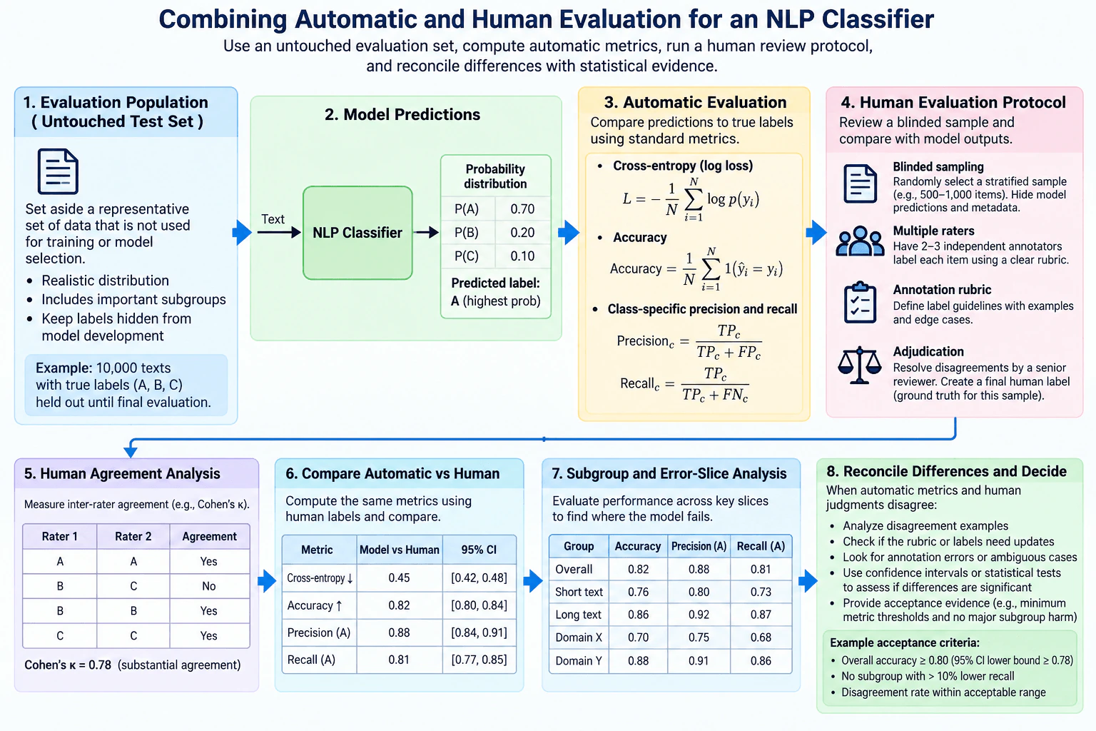
How would you combine automatic and human evaluation for an NLP classifier? diagram
How to Explain It in an Interview

Start with the evaluation population. I would set aside a representative collection of texts that is not used for training or model selection. The diagram uses an illustrative example of 10,000 texts with true labels A, B, and C. The important point is not the number 10,000; it is that the final population stays untouched and contains the important subgroups we care about.

Next, run the classifier on every text. For each text, the model returns a probability distribution over the mutually exclusive labels. The diagram shows an example with P(A) = 0.70, P(B) = 0.20, and P(C) = 0.10, so A is the predicted class because it has the highest probability.

Then compute automatic metrics. Cross-entropy, also called log loss, uses the probability assigned to the true class. For N examples, it can be written as L = -(1/N) * sum(log(p(y_i))), where p(y_i) is the probability assigned to the true label of example i. Lower cross-entropy is better. Accuracy is the fraction of examples whose predicted class equals the true class. I would also report precision and recall separately for each class. Precision for class c is TP_c / (TP_c + FP_c), and recall for class c is TP_c / (TP_c + FN_c). Per-class metrics matter because overall accuracy can hide a weak class.

In parallel, I would create a human review protocol. I would define an annotation rubric with clear label definitions, examples, and edge cases. I would draw a random or appropriately stratified sample from the untouched evaluation population. The diagram gives 500 to 1,000 items only as an example sampling size, not as a universal requirement. Reviewers should be blinded to model predictions and unnecessary model metadata so that the model does not influence their judgment.

I would have multiple independent annotators review each sampled item. The diagram uses two to three raters as an example. For two raters, Cohen's kappa is one reasonable agreement statistic because it adjusts observed agreement for chance agreement. The diagram's kappa value of 0.78 is an illustrative result, not a claimed experiment result. If more than two raters are evaluated jointly, I would use an agreement statistic designed for multiple raters instead of treating a two-rater Cohen's kappa as the joint agreement measure.

Disagreements should go through adjudication. A senior reviewer examines the disputed cases using the same rubric and creates a final human label for the reviewed sample. I would keep the disagreement examples because they often expose ambiguous language, rubric gaps, noisy reference labels, or systematic model errors.

After adjudication, I would compare the classifier with the adjudicated human labels on the reviewed sample. I would compute the relevant metrics and report uncertainty, such as 95% confidence intervals. The values shown in the diagram, including cross-entropy 0.45, accuracy 0.82, precision for A of 0.88, recall for A of 0.81, and their intervals, are illustrative examples rather than measured results from a supplied dataset.

I would then perform subgroup and error-slice analysis. The diagram illustrates slices such as short text, long text, Domain X, and Domain Y. The real slices should come from the actual evaluation population. I would compare accuracy and per-class precision and recall across those slices and inspect recurring error types. A strong overall metric does not compensate for a severe failure in an important subgroup.

Finally, I would reconcile disagreements between automatic metrics and human judgments instead of choosing whichever result looks better. I would inspect disagreement examples, check whether the rubric or reference labels need correction, look for ambiguous inputs, and use confidence intervals or appropriate statistical tests to determine whether differences are meaningful. If the human rubric changes, I would document that change and re-evaluate rather than silently moving the target.

The acceptance rule should be agreed before examining the final results. The diagram gives illustrative criteria: overall accuracy at least 0.80 with the 95% confidence-interval lower bound at least 0.78, no subgroup having more than 10% lower recall, and a disagreement rate within an agreed acceptable range. Those numbers are examples, not universal thresholds. The real decision should require acceptable automatic metrics, credible human-review evidence, sufficient rater agreement, no unacceptable subgroup harm, and a documented explanation for meaningful disagreements. If that evidence is not strong enough, I would refine the rubric or model and evaluate again without repeatedly tuning against the untouched final population.

Technical Approach
  1. Define a representative untouched evaluation population and keep it out of training and model selection.
  2. Run the classifier on that population and retain the complete probability distribution and predicted class for each text.
  3. Compute cross-entropy, overall accuracy, and precision and recall separately for each class.
  4. Define a human annotation rubric with label definitions, examples, and edge cases.
  5. Draw a blinded random or appropriately stratified review sample from the same evaluation population.
  6. Have multiple annotators label each sampled text independently without seeing the model prediction.
  7. Measure inter-rater agreement and send disagreements through adjudication to obtain final human labels for the reviewed sample.
  8. Compare model predictions with the adjudicated human labels and report confidence intervals for the important metrics.
  9. Break results down by important subgroups and error slices and inspect disagreement examples.
  10. If automatic and human evidence disagree, investigate label quality, ambiguity, rubric gaps, and model failure modes rather than relying on one metric alone.
  11. Apply predeclared acceptance criteria using automatic performance, uncertainty, human agreement, subgroup behavior, and the explanation of disagreements.
  12. If the evidence is insufficient, update the rubric or model as appropriate and re-evaluate without repeatedly tuning on the untouched final population.
Practical Insights

Automatic evaluation is cheap and repeatable once predictions and labels exist, so it scales well to the full evaluation population. Human evaluation is slower and more expensive because several people may review the same item and disagreements need adjudication. A larger human sample usually gives narrower uncertainty intervals but increases annotation cost. More raters can provide stronger agreement evidence but also increase time and cost. Cross-entropy uses the full probability distribution and can expose overconfident mistakes, while accuracy only checks the final class. Per-class precision and recall expose class-specific errors that an overall score may hide. Subgroup analysis adds more comparisons, so small slices may have wide confidence intervals and need cautious interpretation.

Why Interviewers Ask This

This tests whether I can design a trustworthy final evaluation instead of relying on one score. I should understand probability-based and label-based metrics, protect an untouched evaluation population, design reproducible human annotation, measure rater agreement, examine important subgroups and error slices, quantify uncertainty, and make a defensible acceptance decision when automatic metrics and human judgments do not tell the same story.

Common interview mistakes

Common mistakes are using the final evaluation population during model selection; reporting only accuracy; ignoring the probability distribution and therefore cross-entropy; reporting aggregate results without class-specific precision and recall; letting human reviewers see model predictions; using an unclear rubric; relying on one annotator; using an agreement statistic that does not match the number of raters; failing to adjudicate disputed labels; ignoring subgroup and error-slice failures; presenting example thresholds or metric values as universal requirements; omitting confidence intervals; and accepting the model simply because automatic metrics are strong when human review reveals a systematic problem.

Interview tip

Present this as one evidence pipeline: untouched population, automatic metrics, blinded human review, agreement and adjudication, subgroup analysis, uncertainty, then a predeclared acceptance decision. Make it explicit that the human and automatic evaluations complement each other rather than compete.
Interviewer may ask next
What would you do if the annotators have low agreement on the human-review sample?

I would not treat the human labels as reliable ground truth yet. I would inspect the disagreement cases and check whether the label definitions are ambiguous, important edge cases are missing, or the task itself has genuinely subjective examples. I would refine the rubric using those findings, train or calibrate the annotators on the clarified rules, and repeat an independent blinded agreement check. Disputed evaluation items would still go through adjudication. I would document the rubric version because changing the rubric changes what the evaluation target means.

What if overall accuracy is acceptable but human review finds poor recall for one important subgroup?

I would not accept the model based on overall accuracy alone. I would quantify the subgroup recall and its uncertainty, inspect the false negatives, and determine whether the gap is caused by model behavior, label quality, ambiguous text, or an unsuitable rubric. I would compare the result with the predeclared subgroup acceptance rule. If the subgroup failure is outside the acceptable range, the evidence is not sufficient for acceptance even when the aggregate metric looks good. I would correct the underlying issue and re-evaluate without tuning repeatedly on the untouched final population.

2. Evaluate threshold choices for a severely imbalanced classifier on twelve scored examples.NEWModel Evaluation And ValidationMediumAmazon

Question Details

The scored records (id,label,score) are A(1,.92), B(0,.90), C(0,.88), D(0,.70), E(1,.62), F(0,.58), G(0,.55), H(0,.54), I(1,.53), J(0,.50), K(0,.20), and L(0,.10). Treat score greater than or equal to the threshold as positive. Compute precision, recall, and F1 at 0.90, 0.60, and 0.50; identify the F1-maximizing threshold; explain how asymmetric costs could change it; compare PR and ROC interpretation at about 1% prevalence; and compute precision@2 and recall@2 while distinguishing ranking from probability calibration.

Short Interview Answer (30-60 seconds)

At 0.90, 0.60, and 0.50, the F1 scores are 0.40, 0.50, and about 0.46, so 0.60 is best among those choices. Lower thresholds favor recall, higher thresholds are more selective, and top-2 precision and recall are 0.50 and about 0.33.

Detailed Explanation

Each record has a binary label and a model score. The task is to turn those scores into positive or negative decisions using score >= threshold, then compare three thresholds with precision, recall, and F1. There are three actual positives: A, E, and I. I will count TP, FP, FN, and TN at each threshold, choose the best F1 among the requested values, and then explain why business error costs may prefer another threshold. I will also compare PR with ROC at about 1% prevalence and separate top-k ranking from probability calibration.

Useful Questions to Ask the Interviewer
  1. Are false negatives and false positives equally costly, or is one type of error more important?
  2. Is the main goal a binary decision, a ranked review queue, or reliable probability estimates?
  3. Should I treat the stated 1% prevalence as the deployment prevalence rather than the prevalence of this twelve-record toy example?
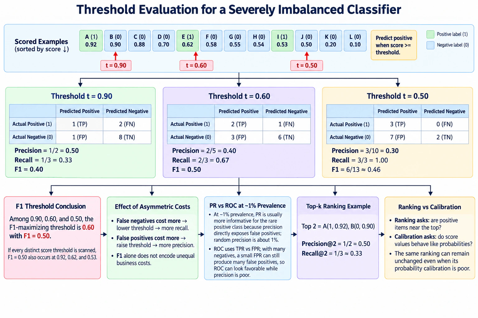
Evaluate threshold choices for a severely imbalanced classifier on twelve scored examples. diagram
How to Explain It in an Interview

The records are already sorted from highest score to lowest score: A(1,.92), B(0,.90), C(0,.88), D(0,.70), E(1,.62), F(0,.58), G(0,.55), H(0,.54), I(1,.53), J(0,.50), K(0,.20), L(0,.10).

There are 3 actual positives, A, E, and I, and 9 actual negatives. The prediction rule is score >= threshold means predicted positive.

At threshold 0.90, the predicted positives are A and B. A is a true positive and B is a false positive. E and I are false negatives. Therefore TP=1, FP=1, FN=2, and TN=8. Precision = TP/(TP+FP) = 1/2 = 0.50. Recall = TP/(TP+FN) = 1/3 ≈ 0.33. F1 = 2PR/(P+R) = 0.40.

At threshold 0.60, the predicted positives are A, B, C, D, and E. A and E are true positives. B, C, and D are false positives. I is the only false negative. Therefore TP=2, FP=3, FN=1, and TN=6. Precision = 2/5 = 0.40. Recall = 2/3 ≈ 0.67. F1 = 0.50.

At threshold 0.50, the predicted positives are A through J because J has score exactly 0.50 and the rule uses >=. A, E, and I are true positives. The other seven predicted-positive records are false positives. Therefore TP=3, FP=7, FN=0, and TN=2. Precision = 3/10 = 0.30. Recall = 3/3 = 1.00. F1 = 2 × 0.30 × 1.00 / (0.30 + 1.00) = 6/13 ≈ 0.46.

Among the three requested thresholds, 0.60 maximizes F1 with F1 = 0.50. If every distinct score is also considered as a possible threshold, the maximum F1 is still 0.50 but is not unique. It also occurs at thresholds 0.92, 0.62, and 0.53. Threshold 0.60 produces the same predicted-positive set as 0.62 because there is no score between 0.60 and 0.62.

The best threshold can change when false-positive and false-negative costs are unequal. F1 balances precision and recall but does not directly encode a business cost ratio. If false negatives are more costly, I would generally lower the threshold so that more records are predicted positive and recall can increase. This usually accepts more false positives. If false positives are more costly, I would generally raise the threshold to make positive predictions more selective, usually trading some recall for better precision. If the costs are known, I would select the threshold using expected cost or expected utility instead of F1 alone.

At about 1% positive prevalence, the precision-recall view is especially useful for understanding the rare positive class. Precision answers: of the records predicted positive, what fraction is actually positive? At 1% prevalence, predicting every record positive gives about 1% precision, so roughly 1% is the natural no-skill precision level. ROC instead compares true-positive rate with false-positive rate. ROC is still useful for discrimination, but when negatives greatly outnumber positives, even a small false-positive rate can create many false positives. That means ROC performance can appear strong while operational precision remains poor.

For top-k ranking, the top two records are A(1,.92) and B(0,.90). One of those two records is actually positive, so precision@2 = 1/2 = 0.50. There are three positives in the full set and the top two contain one of them, so recall@2 = 1/3 ≈ 0.33.

Ranking and probability calibration answer different questions. Ranking asks whether positive records appear near the top when records are ordered by score. Calibration asks whether score values behave like probabilities when the scores are intended to represent probabilities. For example, among many cases assigned a calibrated probability near 0.80, about 80% should actually be positive. A monotonic transformation can preserve the ordering of all records while changing the numerical score values, so ranking can remain unchanged even when probability calibration is poor.

Technical Approach
  1. Keep the records sorted from highest score to lowest score.
  2. For each requested threshold, predict positive for every record with score >= threshold.
  3. Count TP, FP, FN, and TN.
  4. Compute precision = TP/(TP+FP), recall = TP/(TP+FN), and F1 = 2PR/(P+R).
  5. Compare F1 across 0.90, 0.60, and 0.50.
  6. Separately consider whether unequal false-positive and false-negative costs justify a different threshold.
  7. At severe class imbalance, interpret PR together with ROC and pay close attention to precision.
  8. For top-k evaluation, inspect the first k ranked records and compute precision@k and recall@k.
  9. Evaluate ranking and probability calibration as separate properties.
Practical Insights

For twelve records, the computation is tiny. More generally, sorting n records by score costs O(n log n). After sorting, threshold statistics can be updated in one O(n) scan. The important tradeoff is statistical rather than computational. Lowering the threshold can increase recall because more records are called positive, but it can also add false positives. Raising the threshold is more selective and can reduce false positives, but it can miss positives. F1 is useful when precision and recall should receive similar importance, but it does not represent unequal error costs. With about 1% prevalence, false positives can dominate the predicted-positive set, making precision especially important. Calibration also requires enough observations across score ranges to judge whether probability values match observed frequencies.

Why Interviewers Ask This

This question tests whether I can convert continuous model scores into thresholded decisions, calculate precision, recall, and F1 correctly, and reason about severe class imbalance. It also tests whether I understand that the best operating threshold depends on error costs, that PR and ROC emphasize different aspects of classifier performance, and that ranking quality is different from probability calibration.

Common interview mistakes

Common mistakes are using score > threshold instead of the required score >= threshold rule; forgetting that A, E, and I are the only three positives; excluding J at exactly 0.50; miscounting the predicted-positive records at 0.60; comparing thresholds using accuracy instead of the requested precision, recall, and F1; saying 0.60 is the unique global F1 optimum even though other distinct score thresholds also achieve F1=0.50; assuming precision must move monotonically when the threshold changes; treating F1 as if it already represents unequal error costs; saying ROC is invalid for imbalanced data instead of explaining why PR is often more operationally informative; confusing precision@2 with threshold precision; and assuming good ranking automatically means the scores are well calibrated probabilities.

Interview tip

Start with TP, FP, FN, and TN for each threshold, then calculate the three requested metrics. State that 0.60 wins among the requested thresholds. Finish by separating thresholded classification, asymmetric business costs, PR versus ROC under rare prevalence, top-k ranking, and probability calibration.

Interviewer may ask next
If you can choose any distinct score as the threshold instead of only 0.90, 0.60, and 0.50, is 0.60 still the unique F1-maximizing threshold?

No. The maximum F1 is still 0.50, but it is not unique. At threshold 0.92, only A is predicted positive, so precision=1.00, recall=1/3, and F1=0.50. At threshold 0.62, A through E are predicted positive, giving TP=2, FP=3, precision=2/5, recall=2/3, and F1=0.50. At threshold 0.53, A through I are predicted positive, giving TP=3, FP=6, precision=1/3, recall=1.00, and F1=0.50. Threshold 0.60 also gives F1=0.50 because it creates the same predictions as threshold 0.62.

If a false negative costs ten times as much as a false positive, which of the three requested thresholds would you prefer?

Using the simple relative cost function 10 × FN + 1 × FP, threshold 0.90 has cost 10×2 + 1 = 21. Threshold 0.60 has cost 10×1 + 3 = 13. Threshold 0.50 has cost 10×0 + 7 = 7. Under that stated cost rule, I would choose 0.50 even though its F1 is lower than 0.60, because avoiding false negatives is much more valuable.

3. Design an end-to-end NLP classification system for routing customer messages.Machine Learning System DesignEasyAmazon

Question Details

Define the label taxonomy, observation unit, prediction-time boundary, rare-class costs, and whether predictions automate an action or enter human review. Design ingestion, annotation and adjudication, leakage-safe text preprocessing, baselines and candidate models, versioned features and datasets, training and calibration, registry and approval gates, online or batch serving, thresholds and abstention, latency and fallback behavior, per-class and human evaluation, error analysis, feedback and retraining, drift and label-quality monitoring, privacy, access control, audit logs, reliability, and cost.

Short Interview Answer (30-60 seconds)

I would classify one customer message when it arrives, using only information available at that time. I would build versioned, adjudicated labels, compare a TF-IDF plus logistic-regression baseline with a fine-tuned pretrained transformer, calibrate confidence, and apply class-specific thresholds. High-confidence cases auto-route, while uncertain cases abstain to human review, with monitoring and feedback driving future retraining.

Detailed Explanation

The prediction unit is one customer message, and the goal is to route it to the correct team when the message arrives. I would define a versioned routing taxonomy, especially rare or critical classes where a wrong route has higher cost. Human annotation and adjudication create trustworthy labels. The labeled data is then split safely before fitting learned transforms or models. Preprocessing uses only prediction-time-available fields and stays aligned with the chosen model. I would compare a simple baseline with a pretrained transformer, calibrate confidence, and use class-specific thresholds so uncertain cases go to human review.

Useful Questions to Ask the Interviewer
  1. What routing labels exist today, and are any classes rare, critical, or especially costly to misroute?
  2. Is the prediction unit exactly one incoming customer message, or can the model use earlier conversation context?
  3. Should high-confidence predictions automatically route messages, or should predictions always enter human review?
  4. What text and metadata are guaranteed to be available when the message arrives, and which fields are sensitive?
  5. Is the primary serving path real-time online inference, or is separate batch inference also required?
  6. What end-to-end latency, availability, and reliability expectations should the routing path meet?
  7. How quickly do human-reviewed or downstream routing outcomes become available for evaluation and retraining?
  8. What privacy, retention, access-control, and audit requirements apply?
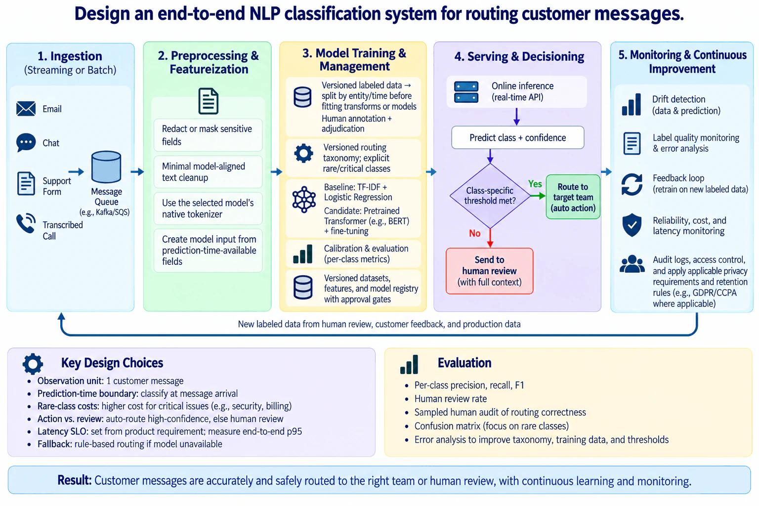
Design an end-to-end NLP classification system for routing customer messages. diagram
How to Explain It in an Interview
1. Define the prediction unit and decision

I would define one observation as one customer message. The prediction-time boundary is message arrival. The model may use the message text and permitted metadata that already exist at that moment, but it must not use information created after routing, such as a later human resolution.

The model returns a routing class and confidence. The business action is separate from that prediction. If the confidence meets the threshold for the predicted class, the message is automatically routed to the target team. Otherwise, the system abstains and sends the message with its available context to human review.

Rare or critical classes need explicit treatment because their mistakes can have different costs. A critical class may need a more conservative decision threshold than a common low-risk class. I would therefore choose thresholds by class rather than assume one global cutoff is appropriate for every route.

2. Ingest messages through a stable contract

Messages may arrive through channels such as email, chat, support forms, or transcribed calls. A queue or equivalent buffering layer can decouple producers from downstream processing and support streaming or batch ingestion.

Each accepted record should preserve a message identifier, event time, permitted content, and the fields required by the model and audit trail. Duplicate, empty, malformed, or unsupported records should be detected before inference so they do not silently create duplicated predictions or inconsistent training examples.

3. Create trustworthy, versioned labels

The routing taxonomy should be versioned because business definitions and team ownership can change. Annotation guidance should define each class clearly, including ambiguous boundaries and rare or critical classes.

Human annotators label examples, and disagreements go through adjudication. This produces a controlled labeled dataset instead of assuming that every historical route is perfect ground truth. Label-quality monitoring should continue after launch because inconsistent annotation can reduce model quality even when the incoming text distribution has not changed.

4. Prevent leakage and training-serving skew

After labeling, I would split the versioned dataset by the appropriate entity or time boundary before fitting learned transforms or models. This prevents duplicate entities or future information from leaking into validation or test data.

Before modeling, I would redact or mask sensitive fields that should not be exposed to the model. Text cleanup should be minimal and model-aligned rather than applying a generic rule such as unconditional lowercasing. For a pretrained transformer, I would use that selected model's native tokenizer.

The final model input should contain only fields available at prediction time. The same preprocessing and feature definitions should be used in training and serving so the system does not create training-serving skew.

5. Build a baseline and a stronger candidate

I would start with a TF-IDF plus logistic-regression baseline. It is fast, inexpensive, interpretable, and gives a useful reference point.

Then I would compare it with a fine-tuned pretrained transformer such as BERT when better language understanding may justify additional complexity. I would not choose the transformer simply because it is more sophisticated. The candidate must improve the routing evaluation that matters while still fitting latency, reliability, and cost requirements.

Datasets, feature definitions, preprocessing configuration, model artifacts, and evaluation results should be versioned. The approved artifact should be stored in a model registry with its lineage so serving loads a known model version rather than an untracked file.

6. Calibrate, evaluate, and approve

Training produces class scores or probabilities, but raw probabilities are not automatically reliable confidence estimates. I would evaluate calibration and calibrate the selected model when needed before using confidence to control automatic routing.

Evaluation should be per class, not just one aggregate number. I would inspect precision, recall, and F1 for each route, with special attention to rare or critical classes. A confusion matrix shows which classes are being mixed up. I would also measure the human-review rate because stricter thresholds usually reduce risky automation but increase manual workload.

A sampled human audit of routing correctness provides another check that offline metrics reflect the real task. Error analysis should look for mislabeled examples, ambiguous taxonomy boundaries, new language patterns, model limitations, preprocessing problems, and threshold mistakes.

The model should pass an approval gate using this broader evidence. I would not deploy a model based only on a training metric.

7. Serve online with class-specific thresholds

The audited design uses online inference as the primary routing path. The service receives prediction-time-safe input and returns a class plus confidence. It then evaluates the threshold for that predicted class.

If the threshold is met, the system routes the message automatically to the target team. If it is not met, the system abstains and sends the case to human review. This is safer than forcing every message into a class.

If the product also requires batch inference, I would implement it as a separate execution path using the same approved model and preprocessing contract. I would not mix batch and online execution semantics into one path.

8. Treat latency as an end-to-end requirement

The latency SLO should come from the product requirement rather than be invented during system design. I would measure end-to-end p95 latency because queueing, preprocessing, network calls, model inference, thresholding, and downstream routing all contribute to the time the customer-facing workflow experiences.

Model execution time is therefore only one part of latency. Monitoring should distinguish a slow model from queueing, dependency, or routing delays.

9. Design safe fallback behavior

If the model path is unavailable, the diagram uses rule-based routing as the fallback. If a rule cannot route the message safely, the system should fall back to human review rather than pretend an ML prediction succeeded.

Timeouts, overload, missing model artifacts, and dependency failures are service-health problems. They should be handled separately from model-quality problems. Keeping a previous approved model artifact in the registry also supports recovery if a newly approved version causes operational or quality problems.

10. Monitor the full production loop

I would monitor data and prediction drift, label quality, routing errors, human-review rate, reliability, latency, and cost. Drift should trigger investigation, not automatically imply that prediction quality declined.

Human review, customer feedback, and production outcomes create new labeled evidence. Those outcomes should be joined back to the original message and prediction using the correct message identifier and time boundary so feedback is not attached to the wrong example.

Error analysis can then determine whether the main issue is taxonomy design, label quality, changed language, model limitations, or thresholds. Retraining should use versioned new labeled data and repeat evaluation, calibration, registry, and approval before a new model replaces the current approved artifact.

11. Protect sensitive data and control access

Sensitive information should be minimized, redacted, or masked when appropriate. Access to raw messages, labeled datasets, model artifacts, and audit records should follow applicable privacy and retention requirements. Access controls should restrict who or what can view or modify protected resources, and audit logs should record important accesses and changes.

Applicable privacy requirements depend on the deployment context. Regulations such as GDPR or CCPA should be followed where they apply rather than assumed to apply universally.

12. Balance quality, automation, reliability, and cost

Cost comes from ingestion, storage, annotation, training, inference, monitoring, and human review. A transformer may improve difficult classifications but require more compute and increase latency or serving cost. Conservative class-specific thresholds can reduce incorrect automatic routes but increase the human-review workload.

The final design therefore balances per-class routing quality, automation rate, human-review cost, end-to-end latency, reliability, privacy, and infrastructure cost instead of optimizing one model metric in isolation.

Technical Approach
  1. Define one customer message as the prediction unit, the routing taxonomy, prediction-time boundary, rare-class costs, and the auto-route versus human-review policy.
  2. Ingest messages through a stable streaming or batch contract and handle duplicate, empty, malformed, or unsupported inputs explicitly.
  3. Create a versioned routing taxonomy and produce labels through human annotation and adjudication.
  4. Split the versioned labeled data by the appropriate entity or time boundary before fitting learned transforms or models.
  5. Redact or mask sensitive fields, apply minimal model-aligned text cleanup, use the selected model's native tokenizer, and restrict model inputs to prediction-time-available fields.
  6. Train a TF-IDF plus logistic-regression baseline and compare it with a fine-tuned pretrained transformer.
  7. Evaluate per-class precision, recall, F1, confusion patterns, human-review rate, and sampled human routing correctness; calibrate confidence when needed.
  8. Version datasets, features, preprocessing configuration, model artifacts, and evaluation evidence, and register only models that pass approval gates.
  9. Serve the approved model through the primary online inference path; use a separate batch inference path only when the product requires asynchronous scoring.
  10. Apply class-specific thresholds: auto-route when the threshold is met and abstain to human review otherwise.
  11. Measure end-to-end latency and reliability, and use rule-based routing or human review when the model path is unavailable.
  12. Monitor drift, label quality, routing errors, human-review rate, latency, reliability, privacy controls, audit logs, and cost.
  13. Join reviewed outcomes and feedback to the original message and prediction, retrain on versioned new labeled data, and repeat calibration, evaluation, registry, and approval before promotion.
Practical Complexity & Trade-offs

The TF-IDF plus logistic-regression baseline is usually cheaper to train and serve and is easier to inspect. A pretrained transformer can understand language better in difficult cases, but it usually needs more compute and can increase serving latency and cost. Conservative class-specific thresholds reduce risky automatic routing but send more messages to human review, which raises manual cost. Looser thresholds increase automation but may increase misroutes. Annotation, versioning, privacy controls, monitoring, and audit logs also add storage and maintenance work, but they make the system safer and reproducible. End-to-end latency matters more than model time alone because queueing, preprocessing, networking, and routing also consume time.

Where it is used

This design is useful when incoming customer messages must be assigned to different support or operations teams from text. It fits systems receiving email, chat, support-form messages, or transcribed calls. It is especially useful when some routing classes are rare or expensive to misclassify, when uncertain cases can be reviewed by people, and when those reviews can later become labeled feedback for model improvement.

Why Interviewers Ask This

This question tests whether I can design the complete lifecycle of an NLP classifier rather than focus only on model training. I need to define the prediction unit and decision boundary, create reliable labels, prevent leakage, choose a sensible baseline and candidate model, calibrate confidence, design safe serving and abstention, evaluate rare classes, and close the loop with monitoring and human feedback. It also tests operational judgment around latency, fallback behavior, privacy, access control, auditability, reliability, model approval, and cost.

Common interview mistakes

Common mistakes are using one global confidence threshold for classes with very different error costs; forcing every message into a class instead of allowing abstention; splitting data in a way that leaks duplicate entities or future information; fitting learned preprocessing before the train-validation split; using fields unavailable when the message arrives; applying generic lowercasing or tokenization that does not match the selected pretrained model; evaluating only aggregate accuracy; ignoring rare-class precision and recall; treating historical routes as perfect labels without adjudication; promoting a model from training metrics alone; measuring only model execution time instead of end-to-end latency; treating drift as proof that model quality declined; retraining without correctly joining feedback to the original prediction; and ignoring privacy, access control, audit logs, human-review cost, or safe fallback behavior.

Interview tip

Start with the decision boundary: one message arrives, the model predicts a route and confidence, and uncertain cases go to a person. Then walk left to right through labels, leakage-safe preprocessing, baseline and candidate models, calibration, approval, serving, monitoring, and feedback. Emphasize class-specific error costs and explain why abstention, human review, and fallback behavior are part of the ML system rather than afterthoughts.

Interviewer may ask next
How would you handle a rare but high-cost routing class with very little labeled data?

I would first make the class definition and annotation guidance precise because label noise is especially harmful when examples are scarce. I would examine per-class precision and recall rather than rely on aggregate metrics, manually review confusion patterns, and use adjudication for ambiguous examples. For serving, I would choose a conservative class-specific threshold that reflects the higher cost of an incorrect automatic route. If confidence does not meet that threshold, the system should abstain to human review. Those reviewed cases then become carefully labeled feedback for future retraining.

What would you change if the transformer improves routing quality but makes the online path too slow or expensive?

I would compare the quality gain with the end-to-end latency and cost impact instead of selecting the transformer automatically. The TF-IDF plus logistic-regression baseline remains a valid production option if it meets the routing requirement. I could also reduce model complexity or keep more uncertain cases in human review, depending on the product constraint. The final choice should consider per-class quality, human-review workload, latency, reliability, and cost together. Any replacement model would still need calibration, evaluation, registry versioning, and approval before it becomes the serving artifact.

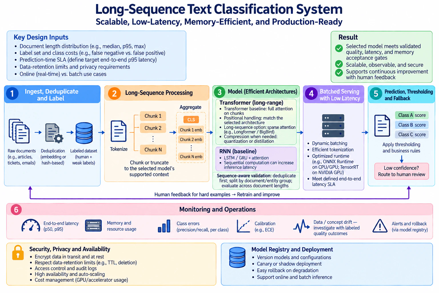
4. Design a long-sequence text-classification system under strict latency and memory limits.Machine Learning System DesignMediumAmazon

Question Details

Define document length distribution, label set, prediction-time SLA, class costs, data-retention limits, and online versus batch use. Design text ingestion, deduplication and labeling; truncation, chunking or hierarchical aggregation; RNN and Transformer baselines with positional and long-range handling; training and sequence-aware validation; model compression or sparse attention where needed; registry, rollout and rollback; tokenization and batched serving; thresholding and fallback; monitoring of latency, memory, class errors, calibration and drift; human feedback and retraining; privacy, security, availability, and accelerator cost.

Short Interview Answer (30-60 seconds)

I would first define document lengths, class costs, retention rules, and the end-to-end p95 latency target. Then I would deduplicate, tokenize, chunk or truncate long documents, compare efficient Transformer and RNN baselines, validate by document groups, serve with dynamic batching and optimized runtimes, and use thresholding, human fallback, monitoring, rollback, and retraining.

Detailed Explanation

The main challenge is preserving useful information from long documents while meeting strict latency and memory limits. I would first measure the document-length distribution and define the label set, class costs, end-to-end p95 prediction latency target, retention rules, and whether predictions are online or batch. Then I would build one consistent pipeline: ingest and deduplicate documents, create labels, tokenize text, chunk or truncate to the selected model's supported context, aggregate chunk evidence when needed, validate without document leakage, and deploy only models that pass quality, latency, and memory acceptance gates.

Useful Questions to Ask the Interviewer
  1. What does the document-length distribution look like at the median, p95, and maximum?
  2. What labels are required, and how do the costs of false negatives and false positives differ by class?
  3. What is the required end-to-end p95 prediction latency, including tokenization and preprocessing?
  4. Which use cases require online predictions, and which can run in batch?
  5. What data-retention and privacy restrictions apply to raw text, labels, predictions, and feedback?
  6. What availability target and accelerator-cost boundary should the design respect?
  7. Is human review an acceptable fallback for low-confidence predictions?
Design a long-sequence text-classification system under strict latency and memory limits. diagram
How to Explain It in an Interview

Start with the design inputs because they determine the architecture. Measure median, p95, and maximum document lengths rather than assuming every document fits one context window. Define the label set and class costs before choosing thresholds. Also define the end-to-end latency SLA, retention limits, privacy requirements, online versus batch use, availability requirements, and accelerator-cost boundary.

For data ingestion, accept raw documents, validate them, and deduplicate them before training or validation. Deduplication reduces the risk that identical or near-identical documents appear on both sides of a split. Keep label provenance when labels come from humans or weak-labeling processes. The prediction remains at document level even if a long document is later divided into chunks.

Next, tokenize with the exact tokenizer expected by the selected model. If a document exceeds the model's supported context, choose between truncation, chunking, or hierarchical aggregation. Truncation is cheapest but can remove important evidence. Chunking retains more text but requires combining chunk-level information. In a hierarchical design, each chunk produces a representation or score and an aggregation step combines those signals into one document-level prediction. Training and serving must use the same tokenization, chunking, and aggregation rules to avoid training-serving skew.

For modeling, establish multiple baselines. A Transformer baseline can use full attention within each chunk. Positional handling must match the selected architecture rather than being added arbitrarily. If long-range information is important and dense attention is too expensive, evaluate a sparse-attention long-sequence architecture such as Longformer or BigBird. If latency or memory is still too high, evaluate compression such as quantization or distillation and revalidate quality. Keep an LSTM or GRU with attention as an RNN baseline. Its recurrent computation is sequential, so it provides less parallelism and can increase inference latency.

Validation must be sequence-aware. Deduplicate first, then split by document or entity group so chunks derived from one source cannot leak across training and validation. Evaluate across document-length slices instead of looking only at an overall average. Measure the quality metrics appropriate to the labels and class costs, including per-class precision and recall, and check calibration, such as expected calibration error when suitable. Do not deploy based only on a training metric. The selected model must pass validated quality, end-to-end latency, and memory acceptance gates.

For serving, keep tokenization and chunking identical to training. Use dynamic batching when the latency budget permits it; batching can improve utilization and throughput, but waiting for a batch can add latency. Use an optimized runtime appropriate to the hardware, such as ONNX Runtime on CPU or GPU, or TensorRT on NVIDIA GPU. Separate model execution time from end-to-end request latency, which also includes tokenization, chunking, aggregation, queueing, and runtime overhead. Online inference should respect the prediction-time SLA, while batch inference can favor larger batches when immediate response is unnecessary.

After inference, apply class thresholds and business rules to the model scores. Thresholds should be chosen from validation results and class costs rather than an arbitrary constant. If confidence is too low and human review is allowed, route the document to review instead of forcing an unreliable automated decision. This creates a safe fallback for hard examples.

Version the model and serving configuration in a model registry. A new model can be introduced through canary or shadow deployment when appropriate. Keep the previous known-good artifact ready so the system can roll back quickly if quality, latency, memory, or service health degrades. The registry and deployment path should support both online and batch inference where the product requires both.

Monitoring should separate service health from model quality. Track end-to-end p50 and p95 latency, memory and resource usage, class-level precision and recall, and calibration. Monitor text and label distributions for data or concept drift, but do not treat drift by itself as proof that model quality has declined. Investigate drift using labeled quality outcomes when they become available. Alerts should connect to operational response and rollback through the model registry when production behavior falls outside accepted limits.

Human-reviewed hard examples can feed back into the labeled dataset. Join feedback to the correct original document and prediction before retraining. The retraining pipeline must repeat deduplication, sequence-aware splitting, document-length evaluation, and the same quality, latency, and memory gates before a new version can be registered and deployed.

Finally, protect the data and service. Encrypt data in transit and at rest, enforce access controls and audit logging, respect retention and deletion requirements, and design serving for high availability and scaling. Accelerator use should be justified by measured latency, memory, throughput, and cost. The final decision is not simply to choose the model with the longest context. Choose the least costly architecture that preserves enough document information while passing validated quality, latency, memory, privacy, security, availability, and operational requirements.

Technical Approach
  1. Measure the document-length distribution and define the label set, class costs, end-to-end p95 latency target, retention rules, privacy requirements, availability needs, online versus batch use, and accelerator-cost boundary.
  2. Ingest documents, validate inputs, deduplicate them, and retain label provenance.
  3. Tokenize with the production tokenizer. For over-length documents, choose truncation, chunking, or hierarchical aggregation based on how much distant context matters.
  4. Train a full-attention Transformer-on-chunks baseline and an RNN baseline. Add a sparse-attention long-sequence option when long-range information is important. Test quantization or distillation only when needed for latency or memory.
  5. Deduplicate before splitting. Split by document or entity group and evaluate across document-length ranges so chunks from one document cannot leak between training and validation.
  6. Select a model using validated model quality, per-class errors, calibration, end-to-end latency, and memory acceptance gates rather than training score alone.
  7. Register the selected model and serving configuration. Use canary or shadow deployment when appropriate and keep the previous version available for rollback.
  8. Serve with consistent tokenization and chunking, dynamic batching where the latency budget permits it, and an optimized runtime such as ONNX Runtime on CPU or GPU or TensorRT on NVIDIA GPU. Keep online and batch inference paths explicit.
  9. Apply validated class thresholds and business rules. Route low-confidence cases to human review when that fallback is permitted.
  10. Monitor end-to-end latency, memory, resource use, class errors, calibration, availability, and drift. Join human feedback to the original prediction and retrain through the same validation gates.
Practical Complexity & Trade-offs

Long text creates a quality-versus-cost tradeoff. Dense self-attention becomes increasingly expensive as sequence length grows, so processing every token together can consume too much memory and time. Chunking reduces the size of each model call, but important evidence can cross chunk boundaries and aggregation adds work. Sparse attention can process longer sequences more efficiently, but it adds architecture complexity. RNN recurrence is sequential and can limit inference parallelism. Dynamic batching can improve hardware utilization and throughput, but waiting to form a batch can increase latency. Quantization can reduce model memory and may improve inference efficiency, while distillation can create a smaller model, but both require quality validation. Human fallback protects difficult cases but adds operational cost and delay. Accelerators can reduce model latency but may increase serving cost. The right choice is the least expensive configuration that still passes the required quality, end-to-end latency, memory, availability, privacy, and security gates.

Where it is used

This design is useful when one prediction must classify a document that may be much longer than a normal model context, such as long reports, support histories, contracts, research documents, policy text, or multi-section records. It is especially useful when some requests require low-latency online predictions while larger offline workloads can run in batches, and when the system must control memory use, accelerator cost, privacy, retention, availability, and low-confidence failures.

Why Interviewers Ask This

This question tests whether a candidate can turn a text classifier into a complete production system when long documents conflict with strict latency and memory limits. It evaluates requirement definition, long-sequence preprocessing, model selection, leakage-resistant validation, serving efficiency, thresholding and fallback, deployment and rollback, monitoring, privacy, availability, and accelerator-cost tradeoffs. A strong answer connects model quality to end-to-end system behavior instead of choosing an architecture only from offline accuracy.

Common interview mistakes

Common mistakes are choosing a long-context model before measuring the document-length distribution; inventing a fixed latency target instead of defining the SLA; allowing duplicate or related documents to cross train-validation boundaries; splitting chunks from the same document independently; using different tokenization or chunking logic in training and serving; truncating without checking whether important evidence is lost; treating ONNX itself as an inference runtime instead of distinguishing the model format from ONNX Runtime; implying TensorRT is a CPU runtime instead of an NVIDIA GPU inference SDK; evaluating only aggregate accuracy while ignoring class costs, per-class errors, calibration, and long-document slices; measuring only model execution time rather than end-to-end latency; forcing a prediction when confidence is too low; treating drift alone as proof of quality loss; deploying without a registry, staged rollout, and rollback path; and collecting human feedback without joining it to the correct original document and prediction.

Interview tip

Lead with the constraints, then make every architecture choice trace back to them. Explain why you chose chunking, sparse attention, compression, batching, thresholds, and fallback instead of listing them independently. Finish with the validation gates, monitoring signals, and rollback path.

Interviewer may ask next
What would you do if the most important evidence often appears in two distant parts of the same document, so independent chunk processing loses context?

I would first verify the failure with error analysis and document-length validation slices. If cross-chunk dependencies are causing the quality loss, simple truncation is not acceptable. I would compare hierarchical aggregation against a sparse-attention long-sequence Transformer such as Longformer or BigBird. A hierarchical model can encode chunks separately and combine their representations into one document-level prediction. A sparse-attention model can connect information across a longer sequence without using dense attention everywhere. I would choose between them using the same validated quality, end-to-end latency, memory, and accelerator-cost gates, while keeping preprocessing identical between training and serving.

What would you change if the latency budget became much tighter but the current model was already close to the required quality?

I would first break end-to-end latency into tokenization, queueing, chunk processing, aggregation, and model execution so I know the real bottleneck. Then I would tune dynamic batching within the new latency budget, use an optimized runtime, and test quantization. If model execution remains the bottleneck, I would compare distillation or a smaller model against the current version. I would reduce the number of processed chunks only if validation shows quality still passes the required gate. Low-confidence predictions can continue to use human review. Every new configuration must pass the same per-class quality, calibration, end-to-end latency, and memory gates before rollout, with the previous model retained for rollback.

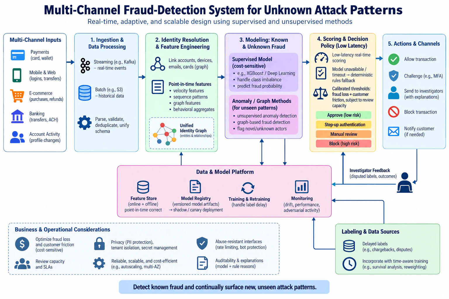
5. Design a multi-channel fraud-detection system that can identify previously unseen attack patterns.Machine Learning System DesignHardAmazon

Question Details

Define transactions and accounts across channels, delayed and disputed labels, review capacity, fraud loss, customer-friction costs, and action tiers. Design streaming and batch ingestion, identity and graph linkage, point-in-time velocity and sequence features, supervised cost-sensitive models plus anomaly or graph methods for unknown actors, calibration and threshold policies, registry and shadow or canary rollout, low-latency scoring and deterministic rules fallback, investigator feedback, drift and adversarial monitoring, retraining under label delay, explanation and auditability, privacy, tenant and secret isolation, abuse-resistant interfaces, reliability, and cost.

Short Interview Answer (30-60 seconds)

I would unify events across channels, resolve accounts and devices into an identity graph, and build point-in-time velocity, sequence, and graph features. I would combine a cost-sensitive supervised model with anomaly and graph methods, then use calibrated thresholds to allow, challenge, review, or block while learning from delayed outcomes.

Detailed Explanation

The system should score activity across payments, mobile and web, e-commerce, banking, and account activity while also finding fraud patterns that were not present in past labels. The key design is to combine known-pattern learning with methods that can surface unusual actors or relationships. Decisions must balance fraud loss against customer friction and limited investigator capacity. Because labels may arrive later through disputes or chargebacks, training and evaluation must respect event time. The serving path must stay low latency, degrade safely when models fail, and keep decisions explainable and auditable.

Useful Questions to Ask the Interviewer
  1. What exactly is the decision unit: each transaction, an account event, or both depending on channel?
  2. Which channels must share identity and risk information, and what identifiers are available for linking accounts, devices, cards, emails, or other entities?
  3. How delayed or disputed are fraud outcomes, and which outcomes are trusted enough to become training labels?
  4. How much manual-review capacity is available, and how should fraud loss be traded against customer friction from challenges or false blocks?
  5. What latency and availability expectations apply to the real-time decision path, without assuming a specific numeric target?
  6. Which privacy, tenant-isolation, secret-management, and audit requirements constrain storage, features, explanations, and interfaces?
Design a multi-channel fraud-detection system that can identify previously unseen attack patterns. diagram
How to Explain It in an Interview
1. Define the prediction and action contract

Treat each incoming transaction or account event as a scoring request at its own event time. The request carries channel-specific information needed for risk assessment plus identifiers that can be linked to the same customer, account, device, card, email, or related entity when available. The output is an action tier: allow, step-up authentication, manual review, or block. Customer notification can follow when appropriate.

Thresholds should minimize expected fraud loss and customer-friction cost while respecting finite review capacity. A manual-review threshold cannot be chosen independently of the number of cases investigators can handle. The supervised risk score should be calibrated before it is used as a probability-like input to the threshold policy.

2. Ingest both live and historical data

Use a streaming path for real-time events and a batch path for historical data. The diagram shows Kafka as an example streaming technology and S3 as an example historical store, but the important design idea is the separation of live and offline flows.

At ingestion, parse and validate records, deduplicate events, and normalize channel-specific schemas. Keep source event time because fraud features and labels are time dependent. Duplicate or invalid events must not silently create extra transactions, graph edges, or inflated velocity counts.

3. Resolve identity across channels

Create a unified identity graph that links entities such as accounts, devices, emails, cards, and other supported identifiers. This graph lets the system recognize shared devices, suspicious connections, or groups of related entities even when a new actor has little direct history.

Identity resolution must be conservative. An incorrect merge can spread risk from one real person or account to another. Store linkage evidence and make graph construction reproducible so training and serving use the same entity definitions.

4. Build point-in-time features

Create velocity features such as recent counts or amounts, sequence features that summarize behavioral ordering, graph features that describe relationships, and broader behavioral aggregates. Every offline training row must use only information that was available at that row's event time. This is a point-in-time join.

That rule prevents leakage. A later chargeback, a future graph edge, or a transaction that happened after the scored event cannot appear in its training features. The online feature path should use the same feature definitions as offline training so the model does not suffer from training-serving skew. The feature store in the diagram represents online and offline access while preserving point-in-time correctness.

5. Combine known-pattern and unknown-pattern detection

Use a supervised cost-sensitive model for fraud patterns represented in historical labels. The diagram uses XGBoost or deep learning as examples. The exact algorithm is less important than training it with class imbalance and decision costs in mind and validating it on time-respecting data.

Run anomaly and graph methods alongside the supervised model to surface previously unseen patterns. Unsupervised anomaly detection can highlight behavior that differs strongly from learned normal patterns. Graph-based detection can expose suspicious networks, shared devices, coordinated actors, or novel relationships. A high anomaly score is evidence for additional risk, not proof of fraud, so it should feed the risk policy rather than automatically force a block.

6. Calibrate scores and choose thresholds by business cost

Calibrate the supervised risk output and combine the available supervised, anomaly, graph, and rule signals through a defined decision policy. Thresholds should reflect fraud loss, customer-friction cost, and review capacity.

Low-risk events can be allowed. Events requiring additional confidence can receive step-up authentication. Uncertain cases that fit investigator capacity can be routed to manual review. Very high-risk cases can be blocked. These tiers should be evaluated using business outcomes, not only model metrics from training.

7. Serve with safe degradation

The online path must perform low-latency real-time scoring using current point-in-time features. Model time is only one part of end-to-end latency; feature retrieval, identity lookup, graph access, request handling, and policy evaluation also contribute.

If the required model is unavailable or scoring times out, use deterministic rules as the fallback rather than pretending the model succeeded. Also define behavior for stale or missing features. A safe fallback should be intentionally conservative and observable because overusing it can either increase fraud loss or create excessive customer friction.

8. Train, validate, register, and deploy safely

Training uses historical events joined to delayed fraud outcomes at the correct entity and time. Version data, code, feature definitions, configuration, model artifacts, and evaluation results needed to reproduce an approved model. The model registry stores versioned model artifacts; deployment is a separate step.

Do not promote a model because of one training metric. Validate it on time-separated data using predictive quality, calibration, business-cost behavior, and the effect on review volume. Introduce a new model through shadow evaluation or a canary rollout so its decisions and operational behavior can be compared before broader exposure. Keep the prior approved artifact available so a bad canary can be rolled back without rebuilding the model.

9. Handle delayed and disputed labels correctly

Fraud outcomes may arrive later through chargebacks, disputes, investigator decisions, or other confirmed outcomes. Store label time separately from event time. Join the eventual outcome back to the original prediction at the correct transaction or account-event grain.

Recent apparently legitimate events may simply be unlabeled because the observation window is incomplete. Retraining must account for that label delay instead of treating every not-yet-disputed event as a clean negative. Time-aware training, mature-label windows, reweighting, or other delay-aware methods can be considered according to the observed label process.

10. Close the investigator feedback loop

Investigators receive selected cases together with explanations or reason codes. Their reviewed decisions, disputed labels, and eventual outcomes flow back into the data and model platform. Feedback must retain the original request, feature or feature-version context, prediction, action, event time, and later outcome so learning and audits stay correctly joined.

Investigator feedback can improve labels, rules, thresholds, and future models, but reviewer decisions should not be treated as automatically perfect. Disagreements and disputed outcomes should remain represented rather than being silently overwritten.

11. Monitor the system in separate layers

Monitor service health such as latency, errors, timeouts, and fallback usage separately from data quality, feature freshness, drift, model quality, adversarial activity, and business outcomes. Drift alone does not prove that model quality has fallen; it is a signal that needs investigation.

For fraud specifically, monitor emerging clusters, changes in graph structure, unusual feature distributions, sudden channel shifts, and behavior that may indicate attackers adapting to the system. Retraining should be driven by mature new labels and demonstrated need, not by drift alerts alone.

12. Make decisions explainable, secure, and auditable

Record reason codes or model explanations for investigator-facing and audit use. Keep an audit trail connecting the request, feature versions, prediction, threshold policy, final action, and eventual outcome.

Protect personally identifiable information, encrypt sensitive data as required by the environment, isolate tenants and secrets, and restrict access to training and serving assets. External and internal scoring interfaces should be abuse resistant through controls such as authentication, authorization, request validation, rate limiting, and bot protection so attackers cannot freely probe the decision boundary.

13. Design for reliability and cost

Scale streaming ingestion, feature computation, graph access, and scoring independently because their workloads differ. Keep online state limited to what is needed for low-latency decisions and move heavier historical work to batch processing where possible. This controls cost without weakening the real-time path.

Reliability includes handling overload, stale features, unavailable models, timeouts, and downstream failures with explicit degradation paths. The final design is successful when it reduces expected fraud loss without creating unacceptable customer friction, stays within review capacity, and continues to surface new attack patterns that supervised labels alone would miss.

Technical Approach
  1. Define the scoring grain, channel inputs, identity keys, delayed-label semantics, action tiers, fraud-loss cost, customer-friction cost, and manual-review capacity.
  2. Ingest live events through a streaming path and historical records through a batch path; validate schemas, deduplicate events, and retain event time.
  3. Resolve identities across accounts, devices, cards, emails, and other supported entities into a unified graph without unsafe merges.
  4. Build shared point-in-time velocity, sequence, behavioral, and graph features for offline training and online serving.
  5. Train a cost-sensitive supervised model for known fraud while using anomaly and graph methods to surface unseen patterns and unknown actors.
  6. Validate on time-separated, label-mature data; check calibration, predictive quality, business cost, and expected manual-review volume rather than relying on a training metric alone.
  7. Register versioned model artifacts and deploy new versions through shadow evaluation or a canary rollout.
  8. During online serving, fetch current features, score with the available models, apply calibrated cost- and capacity-aware thresholds, and return allow, step-up, review, or block.
  9. If a model is unavailable or times out, route the request through the deterministic-rules fallback and record the degraded decision path.
  10. Join delayed chargebacks, disputes, confirmed outcomes, and investigator feedback back to the original predictions at the correct entity and event time.
  11. Monitor service health, data quality, drift, model quality, adversarial behavior, review load, customer friction, and fraud outcomes separately.
  12. Retrain with mature delayed labels when evidence supports it, maintain lineage and auditability, and protect the system with privacy, tenant isolation, secret isolation, and abuse-resistant interfaces.
Time & Space Complexity

The real-time path is expensive because every event may require identity lookup, fresh velocity features, graph information, one or more model scores, and policy evaluation before an action is returned. Graph features can be especially costly if they require large neighborhood traversals, so precomputed or bounded features are often safer for online use. More anomaly sensitivity may find novel attacks earlier but can also increase false alarms and investigator load. Lower thresholds can reduce fraud loss but create more customer friction. Higher thresholds reduce friction but may allow more fraud. Manual review is a hard capacity constraint, so thresholds must control review volume. Keeping online and offline features consistent adds engineering work but prevents leakage and training-serving skew. Delayed labels slow evaluation and retraining because recent examples may not yet have trustworthy outcomes. Shadow and canary rollout increase operational complexity but reduce deployment risk. Privacy controls, audit logs, tenant isolation, secret isolation, and abuse protection add storage and compute cost, but they are necessary parts of a production fraud system.

Where it is used

This design is useful anywhere risk must be assessed across several interaction channels and attackers can change behavior faster than confirmed labels arrive. Examples include payment authorization, account takeover detection, suspicious transfers, refund or return abuse, login and device-risk assessment, and coordinated fraud involving multiple accounts or shared devices.

Why Interviewers Ask This

This question tests whether a candidate can design an end-to-end fraud ML system rather than only choose a model. The interviewer is looking for correct handling of cross-channel identity, delayed labels, point-in-time features, unknown fraud patterns, cost-sensitive decisions, human review capacity, low-latency serving, safe fallback behavior, feedback, retraining, monitoring, explainability, security, reliability, and operational cost.

Common interview mistakes

Common mistakes are using only a supervised classifier and therefore missing novel patterns; treating anomaly scores as proof of fraud; training with features or labels that were unavailable at prediction time; failing to deduplicate events or resolve identities consistently across channels; choosing thresholds from model metrics without fraud-loss, customer-friction, and review-capacity costs; treating recent unlabeled events as legitimate despite label delay; using a model registry as if it were the deployment system; deploying directly without shadow or canary evaluation; letting a scoring timeout fail without an explicit deterministic fallback; mixing service-health, data-quality, drift, model-quality, and business-outcome monitoring into one signal; assuming drift proves quality loss; losing the join between investigator feedback and the original prediction; and ignoring privacy, tenant isolation, secret isolation, auditability, interface abuse, reliability, or operating cost.

Interview tip

Start with the decision and label timing, then draw one left-to-right path: channels to ingestion, identity and point-in-time features, known-plus-unknown modeling, calibrated action tiers, and feedback. Explicitly call out review capacity, delayed labels, deterministic fallback, and why anomaly or graph methods complement rather than replace the supervised model.

Interviewer may ask next
How would you train and evaluate the system when fraud labels arrive late and recent transactions have not had enough time to become disputed?

Keep event time and label time separate. Build training and evaluation sets from examples whose outcome windows are mature enough to be trustworthy, and perform every feature join as of the original event time. Do not treat a recent transaction with no dispute yet as a confirmed negative. Join later chargebacks, disputes, confirmed outcomes, and investigator feedback back to the original prediction grain. For model comparison, use time-separated validation and examine calibration, predictive quality, expected fraud loss, customer friction, and review volume. Retrain when enough mature new labels exist or when other evidence shows the current model needs updating; drift by itself is not proof that retraining will improve quality.

What would you change if the anomaly detector starts sending more cases to investigators but confirmed fraud does not increase?

First separate the signals: check data quality, feature freshness, identity-link changes, drift, service behavior, and the anomaly method itself. A higher anomaly rate does not prove that fraud increased. Measure how those alerts affect confirmed fraud capture, false positives, customer friction, and manual-review capacity. Recalibrate or raise the policy threshold for anomaly-driven review if the marginal cases are not valuable, while keeping the supervised and graph signals available. I would not simply disable unknown-pattern detection, because it still provides coverage against attacks absent from labeled history. Any policy change should be tested through shadow evaluation or a controlled canary before broader rollout.

6. Calculate regional revenue and rank the top three customers in each region.Data EngineeringEasyAmazon

Question Details

Use customers(customer_id, name, region) with unique customer_id and sales(sale_id, customer_id, product_id, order_date, amount) with unique sale_id. Write SQL that first aggregates each matched customer’s total spend, then returns one row per ranked customer containing region, regional total revenue, customer_id, customer total spend, and spend_rank. Use RANK() within each region ordered by customer spend descending, so ties share a rank and a region may return more than three rows when rank 3 is tied. Keep ranks 1 through 3, use an inner join as in the reported task, and avoid a many-to-many inflation. With customers (1,Alice,East), (2,Bob,West), (3,Carol,East) and sales (101,1,P1,2023-01-10,120), (102,2,P2,2023-01-11,250), (103,1,P3,2023-01-12,80), Alice spends 200 in East and Bob spends 250 in West.

Short Interview Answer (30-60 seconds)

I would first aggregate matched sales to one row per customer, calculate regional revenue from those totals, rank customers within each region using RANK() ordered by spend descending, and keep spend_rank <= 3. Ties share a rank, so a region may return more than three rows.

Detailed Explanation

See the Code while reading this explanation.

We need to find how much each customer spent, how much money each region earned, and which customers were the biggest spenders in their region. The customer list tells us where each person belongs, while the sales list tells us how much each purchase was worth. We first add together all purchases for each customer who has a matching sale. Then we add those customer amounts to get each region's total. Finally, we order customers from highest to lowest spending inside their region and keep the first three positions, including ties.

Useful Questions to Ask the Interviewer
  1. Should customers without matching sales be excluded? The task specifies an inner join, so I would exclude them.
  2. Should every customer tied at rank 3 be returned? The task specifies RANK(), so yes.
  3. Should regional revenue use the same matched-customer population as the ranking? I would assume yes because both values come from the same inner-joined sales.
How to Explain It in an Interview

The key is to establish the correct grain before calculating the regional total or ranking. customers has one row per customer_id, while sales has one row per sale_id. I inner join them on customer_id because the task explicitly asks for an inner join. Since customer_id is unique in customers, each matched sale joins to at most one customer row, so the join does not create a many-to-many multiplication.

Next, I group by region and customer_id and sum amount. That produces exactly one row per matched customer, with the customer's total spend. This customer-level result is the safe input for both later calculations.

I calculate regional revenue with SUM(customer_spend) OVER (PARTITION BY region). Because each matched customer appears once at this stage, summing the customer totals produces the matched sales revenue for that region without duplicating values.

I calculate spend_rank with RANK() OVER (PARTITION BY region ORDER BY customer_spend DESC). RANK() gives customers with equal spending the same rank. It can leave gaps after ties, which is the required behavior. Filtering with spend_rank <= 3 therefore keeps ranks 1, 2, and 3 rather than forcing exactly three rows. If several customers tie at rank 3, all of them remain.

The final grain is one row per ranked customer. Each row contains region, regional_revenue, customer_id, customer_spend, and spend_rank.

For the supplied example, Alice has East sales of 120 and 80, so her customer spend is 200. Bob has one West sale of 250, so his customer spend is 250. Carol has no matching sale and is excluded by the inner join. East regional revenue is 200 and Alice is rank 1 in East. West regional revenue is 250 and Bob is rank 1 in West.

No streaming, event-time, watermark, checkpoint, retry, serialization, backfill, partition-storage, retention, or recovery behavior is required for this SQL question. The relevant contracts are the unique customer_id in customers, unique sale_id in sales, the join through customer_id, and the customer-level grain created before the window calculations.

Technical Approach

1. Inner join customers and sales on customer_id. 2. Group by region and customer_id and sum amount to create one row per matched customer. 3. Calculate regional_revenue with a windowed SUM partitioned by region. 4. Calculate spend_rank with RANK() partitioned by region and ordered by customer spend descending. 5. Filter to spend_rank <= 3. 6. Return the requested five columns at one-row-per-ranked-customer grain.

Practical Insights

The join processes the matching customer and sales rows, and the first aggregation combines all sales belonging to each customer. If there are N matched sales, this aggregation processes roughly N sale rows. After aggregation, suppose there are C matched customers. Ranking requires ordering those C customer totals within their regions, which typically costs about O(C log C) overall, although database optimizers may execute it differently by partition. Memory is needed for grouping and window processing. The query is straightforward to maintain because each stage has one clear grain and purpose.

Code
WITH
  customer_spend AS (
    SELECT
      c.region,
      c.customer_id,
      -- Establish the required grain: one row per matched customer.
      -- customer_id is unique in customers, so each sale matches at most one customer row.
      SUM(s.amount) AS customer_spend
    FROM
      customers AS c
      INNER JOIN sales AS s
      -- Use the task's required inner join, excluding customers with no matched sales.
      ON s.customer_id = c.customer_id
    GROUP BY
      c.region,
      c.customer_id
  ),
  ranked_customers AS (
    SELECT
      region,
      customer_id,
      customer_spend,
      -- Customer totals are already at one-row-per-customer grain,
      -- so their sum gives matched regional revenue without duplicate inflation.
      SUM(customer_spend) OVER (
        PARTITION BY
          region
      ) AS regional_revenue,
      -- RANK preserves ties as required; tied rank-3 customers all remain eligible.
      RANK() OVER (
        PARTITION BY
          region
        ORDER BY
          customer_spend DESC
      ) AS spend_rank
    FROM
      customer_spend
  )
SELECT
  region,
  regional_revenue,
  customer_id,
  customer_spend,
  spend_rank
FROM
  ranked_customers
  -- Keep ranking positions 1 through 3, not an arbitrary three physical rows.
WHERE
  spend_rank <= 3
  -- This final ordering is only for deterministic, readable presentation of the result.
ORDER BY
  region,
  spend_rank,
  customer_id;
Why Interviewers Ask This

This question tests whether the candidate can preserve the correct data grain, aggregate customer spending without duplication, calculate a regional total from customer-level results, and use a SQL window function correctly. It also tests understanding of RANK() tie behavior and why filtering to ranks 1 through 3 can return more than three customers in a region.

Common interview mistakes

Common mistakes include ranking individual sale rows before calculating each customer's total spend; joining at a grain that duplicates sales and inflates revenue; using ROW_NUMBER(), which breaks ties instead of sharing a rank; using DENSE_RANK(), whose rank sequence differs from the required RANK() behavior after ties; applying a global LIMIT 3 instead of ranking within each region; using a left join even though the task requires an inner join; and assuming every region must return exactly three rows even when rank 3 is tied.

Interview tip

State the grain first: aggregate to one row per matched customer before applying window calculations. Then explain that regional revenue and RANK() both operate on those customer totals, and explicitly mention that rank-3 ties can produce more than three rows.

Interviewer may ask next
How would the query change if the interviewer wanted exactly three customers per region even when spending amounts are tied?

I would use ROW_NUMBER() instead of RANK() and add a deterministic tie-breaker, such as ORDER BY customer_spend DESC, customer_id ASC. Then filtering to row number <= 3 would return at most three customers per region. The extra tie-breaker makes the selection predictable when customers have equal spend.

How would you include customers who have no sales?

I would change the inner join to a left join and calculate customer spend with COALESCE(SUM(s.amount), 0). That keeps customers with no matching sales and gives them zero spend. Regional revenue and ranking would then be calculated from this expanded customer population. This changes the original requirement, so I would only do it if the interviewer explicitly asks for customers without sales to be included.

7. Count distinct Morse-code representations of lowercase words.CodingEasyAmazon

Question Details

Using Python 3.14, implement def unique_morse_representations(words: list[str]) -> int. Map letters a through z to ['.-','-...','-.-.','-..','.','..-.','--.','....','..','.---','-.-','.-..','--','-.','---','.--.','--.-','.-.','...','-','..-','...-','.--','-..-','-.--','--..']. words contains 0 to 1,000 lowercase-English strings, each of length 0 to 20. Translate each word by concatenating its letter codes and return the number of distinct translations. Do not mutate the input; use only the standard library; target O(total input characters) expected time. Inputs outside this contract need not be handled. Example: unique_morse_representations(['gin','zen','gig','msg']) returns 2.

Short Interview Answer (30-60 seconds)

I would map each lowercase letter to its Morse code and translate every word by concatenating those codes. I would store each completed translation in a Python set because a set keeps only distinct values. After processing all words, I return the size of the set. For the example, gin and zen share one translation, and gig and msg share another, so the answer is 2. The expected time is O(T), with O(T) auxiliary space.

Detailed Explanation

See the Code while reading this explanation.

We receive a list of lowercase English words. Each letter has one fixed Morse-code representation. For every word, we replace its letters with their Morse codes and join those codes into one string. Different words can produce the same final Morse string, so we only want to count each final string once. A set is a good fit because it automatically keeps unique values. After all words are translated, the number of values in the set is the answer.

Useful Questions to Ask the Interviewer
  1. Can I assume every input word contains only lowercase English letters, as stated?
  2. Should an empty input return 0, and should an empty word translate to the empty string?
  3. Can I use Python's standard set type to store distinct translations?
Count distinct Morse-code representations of lowercase words. diagram
How to Explain It in an Interview
1. Understand the input and required output

The input is words: list[str]. There can be from 0 to 1,000 words. Each word has length from 0 to 20 and contains lowercase English letters. We must return one integer: the number of distinct Morse-code translations. We do not change the input list.

2. Choose the algorithm and data structure

I use the given 26-entry Morse-code table. The position of a letter tells me which Morse string to use. I also use a set named seen. Each item in seen is one complete Morse translation of a word. The important rule is that after processing each word, seen contains exactly the distinct translations of all words processed so far.

3. Initialize the state

I create the Morse-code list in a through z order. Then I create seen = set(). Before any word is processed, the set is empty because no translation has been created yet.

4. Walk through the example

The input is ['gin', 'zen', 'gig', 'msg'].

For gin, the letters are translated as g -> --., i -> .., and n -> -.. Concatenating them gives --...-.. The set changes from empty to { '--...-.' }, so its size becomes 1.

For zen, the letters are z -> --.., e -> ., and n -> -.. The final translation is also --...-.. Because that value is already in the set, the set stays the same and its size remains 1.

For gig, the letters are g -> --., i -> .., and g -> --.. The translation is --...--.. This is new, so it is added to the set. The set size becomes 2.

For msg, the letters are m -> --, s -> ..., and g -> --.. Its translation is also --...--.. That value is already present, so the set size remains 2.

The set-size sequence is 0 -> 1 -> 1 -> 2 -> 2. Therefore the function returns 2.

5. Explain why the result is correct

After each word, the set contains exactly one copy of every different Morse translation seen so far. Adding a duplicate translation does not change the set. After the last word, the size of the set is therefore exactly the number of distinct Morse-code representations.

6. Explain the Python implementation

For each character, ord(ch) - ord('a') converts a lowercase letter into an index from 0 to 25. That index selects the correct Morse code. I collect the codes for one word, join them into one string, and add that string to seen. After all words are processed, I return len(seen).

7. Explain complexity and edge cases

Let T be the total number of input characters. Every character is translated once. Building and hashing each completed translation takes time proportional to that word's encoded length, so the total expected time is O(T). The stored translated strings can use O(T) auxiliary space in the worst case. An empty words list returns 0. An empty word translates to ''. Repeated words or different words with the same Morse translation count only once.

Key Insight / Why This Solution Works

The key idea is to convert every word into one complete Morse string and use a set to remove duplicates automatically. The Morse list is stored in a through z order, so ord(ch) - ord('a') gives the correct index for each lowercase letter. After a word is fully translated, its completed string is inserted into seen. The central invariant is that after each word, seen contains exactly the distinct Morse translations of all words processed so far. Therefore len(seen) is the required answer after all words are processed.

Code
def unique_morse_representations(words: list[str]) -> int:
    # Store Morse codes in the same order as letters a through z.
    morse = [
        ".-",
        "-...",
        "-.-.",
        "-..",
        ".",
        "..-.",
        "--.",
        "....",
        "..",
        ".---",
        "-.-",
        ".-..",
        "--",
        "-.",
        "---",
        ".--.",
        "--.-",
        ".-.",
        "...",
        "-",
        "..-",
        "...-",
        ".--",
        "-..-",
        "-.--",
        "--..",
    ]

    # Keep only distinct completed Morse translations.
    seen: set[str] = set()

    # Translate every input word without changing the input list or strings.
    for word in words:
        translated = []

        # Convert each lowercase letter to its Morse code using its alphabet index.
        for ch in word:
            translated.append(morse[ord(ch) - ord("a")])

        # Join the letter codes and add the complete translation to the set.
        seen.add("".join(translated))

    # The set size is exactly the number of distinct translations.
    return len(seen)
Time & Space Complexity

Let T be the total number of characters across all input words. Each character is converted to its Morse code once. Building each completed translation and hashing it for insertion into the set takes time proportional to that word's encoded length. Across all words, the total expected time is O(T). Python set lookup and insertion are O(1) on average once the key's hash is available, but computing the hash of each newly built string takes time proportional to its length. The stored translated strings can use O(T) auxiliary space in the worst case.

Where it is used

This pattern is useful when different inputs can be converted into a standard representation and we need to count or detect unique results. Examples include deduplicating normalized identifiers, grouping equivalent encodings, and counting distinct transformed strings.

Why Interviewers Ask This

This problem checks whether a candidate can translate a simple specification into correct code, choose a set for deduplication, map characters to fixed values, and reason clearly about string construction. It also tests duplicate handling, edge cases such as empty input, input-mutation discipline, and accurate complexity analysis. A strong answer should explain why the set represents exactly the distinct translations and why the expected running time grows with the total number of input characters.

Common interview mistakes

A common mistake is counting translated words in a list without removing duplicates, which would return the number of words instead of the number of distinct translations. Another mistake is using the wrong alphabet offset when indexing the Morse table. Candidates can also compare individual letter codes instead of concatenating the full word translation. It is also easy to claim guaranteed O(T) time even though the solution relies on average-case Python set behavior. Finally, changing values inside the original words list would violate the no-mutation requirement.

Interview tip

State the invariant early: after each word, the set contains exactly the distinct complete translations seen so far. Then walk through the set sizes 0 -> 1 -> 1 -> 2 -> 2 for the given example. This makes both the duplicate handling and the final answer easy to explain.

Interviewer may ask next
How would the solution change if the input contained a very large number of words?

The same set-based algorithm still works. Each word can be translated as it arrives and its completed Morse string can be inserted into the set immediately. The expected processing time remains O(T), where T is the total number of characters processed. The main limitation is memory because the set must keep every distinct translation. In the worst case, the auxiliary space remains O(T).

What is the worst-case behavior of using a Python set here?

Python sets are hash based, so their usual lookup and insertion performance is average-case behavior rather than a strict worst-case guarantee. The stated solution therefore has O(T) expected time. In a pathological case with many hash collisions, set operations can take longer. The algorithm's correctness does not change, but its expected-time guarantee is not the same as a guaranteed worst-case linear-time bound.

8. Return all dictionary sentences that can be formed from a string.CodingMediumAmazon

Question Details

Using Python 3.14, implement def word_break_all(s: str, word_dict: list[str]) -> list[str]. s is a lowercase-English string of length 0 to 20. word_dict contains at most 1,000 unique nonempty lowercase-English words and may be reused; words may be selected more than once. Return every sentence whose space-separated words concatenate exactly to s, in any order, with no duplicates. Return [] when s is empty or no segmentation exists. Do not mutate inputs; use only the standard library. Inputs outside the contract need not be handled. Example: word_break_all('catsanddog', ['cat','cats','and','sand','dog']) may return ['cat sand dog','cats and dog'] in either order.

Short Interview Answer (30-60 seconds)

I would use depth-first search with memoization. I define dfs(i) as all valid sentences that can be formed from s[i:]. At each index, I try every dictionary word that matches there, recursively solve the remaining suffix, and prepend the chosen word. I cache each index so shared suffixes are solved once. The total time and space are output-sensitive and can be exponential because the problem may return exponentially many sentences. The recursion depth is at most O(n).

Detailed Explanation

See the Code while reading this explanation.

We need to split the string into dictionary words and return every valid sentence. The words in each sentence must join together to recreate the original string exactly. A dictionary word may be used more than once. If the string is empty, or no full split works, we return an empty list. For "catsanddog", the two shown answers are "cat sand dog" and "cats and dog". The solution uses recursive search and saves results for each starting position so the same remaining suffix is not solved repeatedly.

Useful Questions to Ask the Interviewer
  1. Can the valid sentences be returned in any order? Yes. The problem allows any order.
  2. Can the same dictionary word be used more than once? Yes. Words may be reused.
  3. What should I return for an empty string or when no complete split exists? Return [].
Return all dictionary sentences that can be formed from a string. diagram
How to Explain It in an Interview
1. Understand the input and output

The function receives a lowercase string s and a list of unique nonempty lowercase dictionary words. We must return every sentence whose space-separated words concatenate exactly to s. We must not change either input.

For the diagram example, s = "catsanddog" and the dictionary contains "cat", "cats", "and", "sand", and "dog". One allowed return value is ["cat sand dog", "cats and dog"]. The opposite order is also valid.

2. Define the recursive state

The key state is dfs(i). It means: return every valid sentence that can be formed from the suffix s[i:].

At index i, the code tries every word in word_set. If s.startswith(word, i) is true, that word matches the string at the current position. The recursion then moves to i + len(word) and solves the remaining suffix.

The result for each index is memoized. This means if two branches reach the same suffix, that suffix is computed once and reused.

3. Handle the base case

Let n = len(s). When i == n, the recursion has consumed the entire string successfully. The function returns [""].

The empty string here is a success marker. It tells the previous recursive call that its current word reaches the end of the input. That previous call then appends only the word, without adding a trailing space.

The outer function separately handles s == "" by returning [], which matches the required contract.

4. Walk through the example

Start with dfs(0) on "catsanddog". Two words match at index 0: "cat" and "cats".

If we choose "cat", we move to dfs(3), whose suffix is "sanddog". The word "sand" matches, so we move to dfs(7). The suffix is now "dog". The word "dog" matches and moves to dfs(10). Index 10 is the end of the string, so dfs(10) returns [""]. The calls then build "dog", "sand dog", and finally "cat sand dog".

If we choose "cats" at index 0, we move to dfs(4), whose suffix is "anddog". The word "and" matches and moves to dfs(7). That state was already solved, so memoization reuses ["dog"]. This produces "and dog" and then "cats and dog".

5. Combine each word with valid suffix sentences

For each matching word, the recursive call returns every valid sentence for the remaining suffix. The code combines the current word with each returned suffix.

If the returned suffix is nonempty, it appends word + " " + suffix. If the returned suffix is empty, the current word is the last word, so the code appends only word.

This keeps spacing correct and produces complete sentences only.

6. Explain why the solution is correct

The invariant is: dfs(i) returns exactly the valid sentences that can be formed from s[i:].

Every branch chooses only a dictionary word that matches at the current index. It then combines that word only with valid sentences from the remaining suffix. The base case succeeds only after the whole string has been consumed. Because every possible matching next word is considered, every valid segmentation is generated. Since the dictionary words are unique and each recursive branch is determined by its sequence of matched words, the algorithm does not create duplicate sentences.

7. Explain complexity and edge cases

Memoization prevents the same starting index from being solved repeatedly, but the number of returned sentences can still be exponential in n. Therefore the total running time is output-sensitive and can be exponential. The stored memoized sentence lists are also output-sensitive and can require exponential space. The recursion depth is at most O(n), and the dictionary set uses additional space proportional to the dictionary contents.

Important cases are an empty input string, no valid segmentation, several valid sentences, and reuse of the same dictionary word.

Key Insight / Why This Solution Works

Use top-down depth-first search with memoization. The recursive state is one index i, where dfs(i) returns all valid sentences that can be formed from s[i:]. At each state, try every word in the dictionary set. If s.startswith(word, i) succeeds, recursively solve the suffix beginning at i + len(word). Then prepend the current word to every valid suffix sentence. The base case dfs(n) returns [""] to mark a successful complete segmentation. Memoization stores the completed result for each index, so shared states such as dfs(7) in the diagram are computed once and reused. The central invariant is that every sentence returned by dfs(i) is made only from dictionary words and concatenates exactly to s[i:].

Code
from functools import lru_cache


def word_break_all(s: str, word_dict: list[str]) -> list[str]:
    # The required contract says an empty input string returns no sentences.
    if not s:
        return []

    # Copy the unique dictionary words into a set without mutating the input.
    # Words remain available because the problem allows them to be reused.
    word_set = set(word_dict)
    n = len(s)

    @lru_cache(None)
    def dfs(i: int) -> list[str]:
        # Reaching the end means the current sequence of words formed all of s.
        # The empty suffix is a success marker for the previous recursive call.
        if i == n:
            return [""]

        # Collect every valid sentence that can be formed from s[i:].
        sentences = []

        # Try every dictionary word as the next word at this exact index.
        for word in word_set:
            if s.startswith(word, i):
                # Recursively generate all valid sentences after this word.
                for suffix in dfs(i + len(word)):
                    if suffix:
                        # More words follow, so add exactly one separating space.
                        sentences.append(word + " " + suffix)
                    else:
                        # This word reaches the end, so do not add a trailing space.
                        sentences.append(word)

        # Memoization stores this complete list for index i before reuse.
        return sentences

    # Build every valid sentence starting from the first character.
    return dfs(0)
Time & Space Complexity

Let n be the length of s. There are at most n + 1 memoized index states. At each reachable state, the code may test dictionary words with startswith, so memoization removes repeated work for the same suffix. However, this problem must return every valid sentence. The number of valid sentences can be exponential in n, and building those strings also takes time. Therefore the total time is output-sensitive and can be exponential. The memoized lists of sentences are also output-sensitive and can use exponential space. In addition, the recursion stack is at most O(n) deep, and word_set stores the dictionary words.

Where it is used

This pattern is useful when software must enumerate every valid way to split a sequence into known tokens. Examples include small dictionary-based tokenization tasks, ambiguous command parsing, phrase segmentation, and generating all legal decompositions of a string. Memoization is especially useful when different choices lead to the same remaining suffix, because that suffix can be solved once and reused.

Why Interviewers Ask This

This problem tests whether you can recognize a recursive decomposition problem with multiple valid answers. The interviewer can see whether you define a useful state, handle the end-of-string base case correctly, generate all results instead of only one, and memoize repeated suffix work. It also checks careful string matching, correct Python recursion, handling reusable dictionary words, avoiding duplicate results, and giving a realistic complexity analysis when the output itself can be exponential.

Common interview mistakes

A common mistake is returning after finding the first valid split even though the problem asks for every sentence. Another is forgetting the i == n success base case, which prevents valid recursive paths from producing an answer. Candidates may also add a space after the final word and create trailing whitespace. Recomputing the same suffix without memoization causes unnecessary repeated work. Removing a word after using it is also wrong because dictionary words may be reused. Finally, do not claim polynomial total time without accounting for the potentially exponential number of returned sentences.

Interview tip

Define dfs(i) before writing the recursion: it returns every valid sentence for s[i:]. Then use the example to point out that both branches eventually reach dfs(7). That makes the value of memoization clear and gives you a simple way to explain the whole solution.

Interviewer may ask next
What would change if you only needed to know whether at least one valid segmentation exists?

I would keep the same index-based recursive state, but dfs(i) would return a Boolean instead of a list of sentences. For each matching word, if the recursive suffix returns True, the current state can immediately return True. Memoization would store one Boolean per index. This removes the cost of constructing every sentence. The running time is bounded by the memoized word-matching work, while the extra state and recursion stack use O(n) index space in addition to the dictionary set. The tradeoff is that the function no longer returns the actual sentence.

What happens if the input has a very large number of valid sentences?

The algorithm still has to build and return all of them because that is the required output. Memoization removes repeated computation of the same suffix, but it cannot remove the cost of producing the results themselves. The number and total size of valid sentences can be exponential, so both total running time and memoized output storage can also become exponential. If the interface were allowed to change, a generator could yield sentences gradually to reduce the need to keep the complete final result in memory, but that would not match the required list[str] return type.

9. Return the Kth positive factor of an integer in ascending order.CodingHardAmazon

Question Details

Using Python 3.14, implement def kth_factor(n: int, k: int) -> int. Inputs satisfy 1 <= n <= 1012 and 1 <= k <= 109. Consider every positive divisor of n exactly once and order the divisors increasingly. Return the one-indexed kth divisor, or -1 when n has fewer than k divisors. Use only the Python standard library, do not mutate caller-owned data, avoid double-counting the square root when n is a perfect square, and target O(sqrt(n)) time with O(sqrt(n)) worst-case auxiliary storage or better. Inputs outside the contract need not be handled. Examples: kth_factor(12, 3) returns 3, and kth_factor(7, 3) returns -1.

Short Interview Answer (30-60 seconds)

I would scan possible divisors only up to the integer square root of n. When i divides n, I store i in a small list and its paired divisor n // i in a large list. I avoid storing the pair twice when n is a perfect square. The small divisors are already increasing, and reversing the large list gives the remaining divisors in increasing order. Then I return the one-indexed k-th factor, or -1. Time is O(sqrt(n)) and auxiliary space is O(sqrt(n)).

Detailed Explanation

See the Code while reading this explanation.

The function receives a positive integer n and a positive position k. We need to find every positive number that divides n with no remainder, place those divisors from smallest to largest, and return the divisor in position k. If there are fewer than k divisors, we return -1. We do not need to try every number up to n. Divisors come in pairs, so checking only through the square root is enough. This matches the required O(sqrt(n)) approach.

Useful Questions to Ask the Interviewer
  1. Can I assume n and k always satisfy the stated input bounds?
  2. Should k be treated as one-indexed, so k = 1 means the smallest divisor?
  3. Is O(sqrt(n)) time with extra storage for the discovered divisors acceptable?
Return the Kth positive factor of an integer in ascending order. diagram
How to Explain It in an Interview
1. Understand the input and required output

The function is kth_factor(n: int, k: int) -> int. The inputs satisfy 1 <= n <= 1012 and 1 <= k <= 109. We need every positive divisor exactly once and in increasing order. We return the divisor at one-indexed position k. If that position does not exist, we return -1.

2. Choose the divisor-pair method

A divisor at or below sqrt(n) has a matching divisor at or above sqrt(n). If i divides n, its pair is n // i. I keep the smaller divisors in small and the paired larger divisors in large. I scan i from 1 through isqrt(n). This avoids scanning all the way to n.

3. Build the ordered divisor lists

I set limit = isqrt(n). For each i from 1 through limit, I check n % i == 0. If true, I append i to small. Then I calculate j = n // i. I append j to large only when j != i. That condition prevents the square root from being counted twice when n is a perfect square.

4. Walk through n = 12 and k = 3

Here limit = isqrt(12) = 3. At i = 1, 12 % 1 == 0, so small = [1] and large = [12]. At i = 2, 12 % 2 == 0, so small = [1, 2] and large = [12, 6]. At i = 3, 12 % 3 == 0, so small = [1, 2, 3] and large = [12, 6, 4]. Reversing large gives [4, 6, 12]. Combining the lists gives [1, 2, 3, 4, 6, 12]. Since k - 1 = 2, factors[2] is 3.

5. Explain why the result is correct

Every positive divisor belongs to a pair i and n // i. Scanning through isqrt(n) finds the smaller member of every divisor pair. small is produced in increasing order. The paired values in large are produced in decreasing order, so reversing large makes them increasing. The j != i check prevents double-counting the square root for perfect squares. Therefore the combined list contains every positive divisor exactly once and in increasing order.

6. Explain the Python implementation

Python's math.isqrt gives the integer square-root boundary without using floating-point arithmetic. The loop finds divisor pairs. small + large[::-1] creates the complete ordered factor list. If k <= len(factors), the one-indexed answer is stored at index k - 1. Otherwise the function returns -1.

7. Explain complexity and edge cases

The loop checks at most about sqrt(n) candidate values, so the time complexity is O(sqrt(n)). The lists and copied reversed slice can use O(sqrt(n)) auxiliary space in the worst case. Important cases are n = 1, a perfect square where the square root must appear once, and k being larger than the total divisor count.

Key Insight / Why This Solution Works

The key insight is that divisors occur in pairs. If i divides n, then n // i is also a divisor. It is enough to test i from 1 through isqrt(n). The invariant is that after each loop iteration, small contains all discovered divisors from the lower side in increasing order, while large contains their distinct paired divisors in decreasing order. When i == n // i, the square-root divisor is stored only once. Reversing large and appending it to small therefore produces every positive divisor exactly once in increasing order.

Code
from math import isqrt


def kth_factor(n: int, k: int) -> int:
    # Store divisors found on the smaller side of each divisor pair.
    small = []

    # Store matching larger divisors. They are discovered in decreasing order.
    large = []

    # Test candidates only through the exact integer square root of n.
    limit = isqrt(n)

    for i in range(1, limit + 1):
        # A zero remainder means i is a positive divisor of n.
        if n % i == 0:
            small.append(i)

            # Compute the divisor paired with i.
            j = n // i

            # For a perfect square, store the square root only once.
            if j != i:
                large.append(j)

    # small is increasing. Reverse large before combining to keep ascending order.
    factors = small + large[::-1]

    # k is one-indexed, while Python list indices are zero-indexed.
    if k <= len(factors):
        return factors[k - 1]

    # Return -1 when n has fewer than k positive divisors.
    return -1


# Verified example from the diagram: kth_factor(12, 3) returns 3.
Time & Space Complexity

The loop checks integers only from 1 through isqrt(n), so the time complexity is O(sqrt(n)). The algorithm stores divisors in small and large. The expression large[::-1] also creates a reversed copy, and the final concatenation creates the complete factors list. All of this extra memory is still O(sqrt(n)) in the worst case. Therefore the auxiliary space complexity is O(sqrt(n)).

Where it is used

This divisor-pair pattern is useful when software needs to enumerate factors of an integer without checking every value up to n. It appears in number-theory utilities, factor-pair calculations, divisibility checks, and problems that need all positive divisors in sorted order.

Why Interviewers Ask This

This problem checks whether you recognize that divisors come in pairs and can reduce a direct scan from O(n) to O(sqrt(n)). It also tests careful ordering, correct handling of perfect squares, one-indexed versus zero-indexed access, and accurate complexity reasoning. The interviewer can see whether you can turn a mathematical observation into clear Python code while preserving the exact output contract and handling edge cases correctly.

Common interview mistakes

A common mistake is scanning all the way to n instead of stopping at the square root. Another is storing both i and n // i when they are equal, which counts a perfect-square root twice. Candidates may also forget that large is discovered in decreasing order and combine it without reversing it. Another mistake is using k directly as a Python list index instead of k - 1. Finally, returning something other than -1 when there are fewer than k divisors breaks the required output contract.

Interview tip

Explain the divisor-pair invariant before writing code. Say that every divisor at or below sqrt(n) gives a paired divisor at or above sqrt(n). Then explain why j != i handles perfect squares and why reversing large produces the final increasing order.

Interviewer may ask next
Can you reduce the auxiliary space if you only need the k-th factor and not the complete sorted divisor list?

Yes. We can avoid storing all divisors by using counting passes. First scan upward from 1 through isqrt(n) and count valid smaller divisors. If the k-th factor is in this lower half, return it when its count reaches k. Otherwise scan downward from isqrt(n) to 1 and consider the paired value n // i, skipping the duplicate square root when needed. Continue the count until position k is reached. This keeps O(sqrt(n)) time and reduces auxiliary space to O(1). The tradeoff is a slightly more complex counting implementation.

What changes when n is a perfect square?

The square root forms a divisor pair with itself. For example, if i * i == n, then i == n // i. That value must be included only once. The current solution already handles this with if j != i before appending j to large. The algorithm still uses O(sqrt(n)) time and O(sqrt(n)) worst-case auxiliary space.

10. Tell me about a time you faced a major difficulty at work. What did you do?BehavioralEasyAmazon

Question Details

Use a real work, internship, research, or academic-team situation. Explain what made the difficulty consequential, what outcome you personally owned, the facts you gathered, the options and trade-offs you considered, the actions you took, how and when you communicated with affected people, the measurable or observable result, and what you learned or would do differently. Keep other people and employers de-identified.

Interview tip:

Use STAR to structure your answer: briefly explain the Situation and Task, make Action the most detailed part, and finish with the Result. For example, describe a difficult analysis where unexpected data quality problems put an important delivery at risk, explain what outcome you personally owned, how you investigated the issue, compared possible solutions, communicated the risk early, chose a practical approach, and delivered a trustworthy result while learning how to detect similar problems sooner.

Situation

In my last role, I was working on an analysis that several stakeholders planned to use for an important business decision. During my final validation, I found that a key data source had inconsistent definitions across different time periods. The numbers looked reasonable at first, so the problem could easily have gone unnoticed, but using them as they were would have made the conclusions unreliable.

Task

I was responsible for determining whether the analysis could still be completed with enough confidence to support the decision. I needed to understand the size of the data problem, decide whether to repair the data or reduce the scope of the analysis, and communicate any impact before stakeholders relied on the results.

Action

I first separated the affected data from the rest of the dataset and traced how the important fields had been created over time. I compared distributions, missing values, and category definitions across periods to identify where the meaning had changed. I also checked the transformation logic so I could distinguish a processing error from a true source data change. Once I understood the issue, I considered two options. One option was to create assumptions that would map the older data into the newer definition. That would preserve more history, but it would add uncertainty that was difficult to validate. The other option was to use only the period where the definition was consistent. That reduced the amount of data but gave us a result I could defend. I recommended the second option because reliability mattered more than having a longer history. I explained the issue to the affected stakeholders as soon as I had enough evidence, showed what part of the analysis was still trustworthy, and made the tradeoff clear rather than simply reporting a delay. I then rebuilt the analysis using the consistent data, added validation checks around the problematic fields, and documented the limitation so the result would not be interpreted more broadly than the evidence supported.

Result

We were able to complete the analysis with a narrower but much more reliable scope, and the stakeholders could make their decision with a clear understanding of the data limitation. The experience taught me that a difficult situation is often best handled by making uncertainty visible instead of trying to hide it with extra assumptions. I also learned to add checks for definition changes earlier in the analysis so similar problems can be found before the final validation stage.

Why Interviewers Ask This

Interviewers ask this question to understand how a candidate behaves when an important piece of work becomes difficult or uncertain. A strong answer shows ownership, calm problem solving, sound judgment about tradeoffs, early communication, and the ability to protect the quality of a decision instead of taking shortcuts under pressure.

Interviewer may ask next
Why did you choose to reduce the scope instead of trying to repair the historical data?

I chose the narrower scope because I could validate it directly. Repairing the historical data would have required assumptions about how old definitions mapped to new ones, and I did not have enough evidence to prove those assumptions were correct. I felt it was better to give stakeholders a smaller result with clear confidence than a broader result with hidden uncertainty.

What would you do differently if you faced the same difficulty again?

I would test for changes in field definitions and data distributions much earlier. In this case, I found the problem during final validation. Now I would make those checks part of the initial data profiling step and confirm important business definitions with the data owners before doing the full analysis. That would surface the risk sooner and give the team more time to decide how to handle it.

More questions load as you scroll

Disclaimer: This interview guide is for educational and informational purposes only. It is designed to help readers prepare, but it does not guarantee any interview result, hiring decision, offer, or outcome. Interview questions, hiring criteria, and preferred answers can vary by employer, interviewer, industry, location, and time. The examples and explanations reflect the authors' research and judgment, are provided without warranties of any kind, and should not be treated as the only correct approach. Diagrams are simplified illustrations intended to highlight the main components and their interactions; actual systems and implementations may be more complex. Alternative approaches may be equally valid or better suited to a particular question, context, or interviewer. To the fullest extent permitted by applicable law, the author, contributors, and publisher are not liable for decisions made, actions taken, or losses incurred based on this guide.

Company Notice: This guide is an independent educational resource and is not affiliated with, endorsed by, sponsored by, or approved by the company named in this guide. Company names are used only to identify interview experiences commonly reported by candidates. Interview practices can change without notice, and inclusion of company-specific content does not mean these questions are official, complete, or guaranteed to be asked. To the fullest extent permitted by law, the author, contributors, and publisher are not responsible for outcomes related to use of this material.

Content Accuracy and Verification: To the fullest extent permitted by applicable law, we do not represent or warrant that interview guides, questions, answers, examples, or diagrams are accurate, complete, current, error-free, or suitable for any particular purpose. You are responsible for independently reviewing and verifying the information before relying on it.