1. What is the downside of evaluating a fitted model only with R-squared?
For a regression model, define the evaluation population, baseline mean prediction, and the exact R-squared calculation. Explain why a high value does not establish causal validity, calibrated errors, useful predictions, stable coefficients, or acceptable behavior under outliers and distribution shift, and why adding predictors can increase in-sample R-squared. Specify residual, holdout, subgroup, robustness, and business-loss checks that must accompany it, including cases where a lower R-squared model is the better production choice.
R-squared tells me how much squared prediction error the model removes relative to predicting the target mean, but it is only one signal. A high value does not prove causality, calibrated errors, stable coefficients, robustness, or good future performance. I would also check residuals, holdout MAE and RMSE, subgroups, outliers, distribution shifts, and business loss.
For a regression model, R-squared compares the model's squared prediction errors with a baseline that always predicts the mean target value in the evaluation population. If the actual targets are y_i, predictions are ŷ_i, and the evaluation-population mean is ȳ, then R² = 1 - Σ(y_i - ŷ_i)² / Σ(y_i - ȳ)². R² = 1 is a perfect fit, R² = 0 matches the mean baseline, and R² can be negative. The downside is that this single number hides many ways a fitted model can fail in practice.
- Which population should the model represent when we evaluate it: the training population, a separate holdout population, or the expected production population?
- Which prediction errors matter most to the real decision, and should MAE, RMSE, or a business-loss metric be the main companion to R-squared?
- Are there important subgroups, time periods, or population shifts that should be checked separately?
- Are outliers expected to be genuine production cases, data-quality problems, or both?
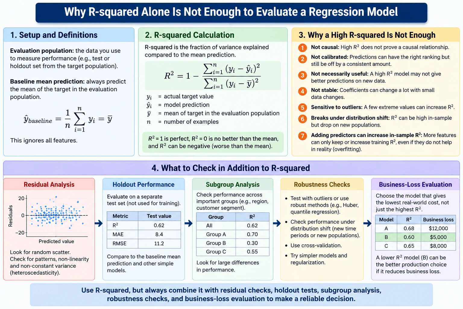
Start with the baseline. For the evaluation population, compute ȳ, the mean of the actual target values. A mean-only predictor ignores the features and returns ȳ for every example. R-squared compares the fitted model's residual sum of squares with the mean baseline's total sum of squares:
R² = 1 - Σ(y_i - ŷ_i)² / Σ(y_i - ȳ)².
Here, y_i is the actual target, ŷ_i is the model prediction, and ȳ is the mean target in the evaluation population. R² = 1 means perfect predictions on those observations. R² = 0 means the model is no better, by this squared-error comparison, than always predicting the mean. R² can also be negative when the model performs worse than that mean baseline.
A high R-squared still does not answer every evaluation question.
First, it does not establish causality. Features can be strongly associated with the target and produce a high R-squared without causing the outcome. Predictive fit and causal validity are different claims.
Second, it does not guarantee well-calibrated errors. A model can have a high R-squared while predictions are systematically too high or too low in part of the range. R-squared summarizes overall squared error relative to the mean baseline; it does not replace checking whether prediction errors have systematic bias or structure.
Third, a high R-squared does not guarantee useful predictions on unseen data. Evaluate a separate holdout or test set that was not used to fit the model. Alongside holdout R-squared, inspect MAE and RMSE. MAE gives the average absolute error, while RMSE gives more weight to large errors. Cross-validation can add evidence about how stable performance is across different train-validation partitions when that procedure is appropriate.
Fourth, inspect residuals, where a residual is actual value minus predicted value. Plot residuals against predicted values and look for random scatter around zero. Curves, changing spread, clusters, or extreme residuals can reveal missing non-linearity, non-constant variance, subgroup structure, or influential observations that one R-squared value hides.
Fifth, one overall R-squared can hide weak subgroup performance. Calculate relevant metrics separately for important groups, such as regions or customer segments when those groups are part of the real evaluation problem. Large differences can show that acceptable aggregate performance hides poor behavior for an important slice of the population.
Sixth, R-squared does not guarantee stable coefficients. In coefficient-based regression models, small data changes or strongly correlated predictors can make coefficient estimates change substantially even when predictive fit remains similar. That matters when coefficients are interpreted or when parameter stability is important.
Seventh, squared-error fitting and evaluation can be sensitive to outliers. Inspect extreme observations and decide whether they are genuine cases, data problems, or both. When appropriate, compare robust approaches such as Huber loss or quantile regression. These methods optimize different objectives, so they should be chosen because they match the prediction goal, not simply because they produce a preferred R-squared.
Eighth, performance can change under distribution shift. A model can perform well on one population or time period and then degrade when the feature distribution or the relationship between features and the target changes. Test plausible shifts, later time periods, or new populations when they represent realistic production conditions.
For nested ordinary least-squares linear regression models evaluated in-sample on the same observations, adding predictors cannot decrease ordinary training R-squared. The larger model can reproduce the smaller model and may reduce the residual sum of squares. Therefore, an added predictor can make training R-squared stay the same or increase even when it adds little real predictive value. A higher in-sample R-squared is not sufficient evidence of better generalization.
Finally, connect statistical evaluation to the real decision. Compare candidate models using residual behavior, holdout R-squared, MAE, RMSE, subgroup performance, robustness under outliers and distribution shift, and a business-loss function that represents the real cost of prediction errors. The best production model is not automatically the model with the highest R-squared. A model with lower R-squared can be the better choice when it gives lower business loss, fewer costly errors, more stable behavior, or better robustness.
- Define the evaluation population: the examples whose prediction quality matters for the decision.
- Compute the target mean ȳ on that evaluation population and use it as the mean-prediction baseline.
- Compute R² = 1 - Σ(y_i - ŷ_i)² / Σ(y_i - ȳ)² on the chosen evaluation data.
- Plot residuals against predicted values and inspect patterns, non-linearity, changing variance, and extreme residuals.
- Evaluate unseen holdout data with R-squared plus direct error metrics such as MAE and RMSE.
- Break the same evaluation down by important subgroups and look for large performance gaps.
- Test plausible outliers and distribution shifts, and use cross-validation or robust methods when they match the problem.
- Compare candidate models using the real business-loss function as well as statistical metrics.
- Choose the model with the most reliable and useful production behavior, even when another model has higher R-squared.
R-squared is cheap and easy to compute, so it is a useful summary metric, but relying on it alone creates evaluation risk. Residual plots, MAE, and RMSE add little computational cost. Holdout testing requires reserving data that cannot be used for fitting or tuning. Cross-validation costs more because the model is fitted several times. Subgroup and distribution-shift checks require enough representative data in each slice. Robust methods can reduce sensitivity to extreme values but optimize a different loss or modeling objective. Business-loss evaluation also requires a defensible way to translate prediction errors into real decision costs. The extra evaluation work is worthwhile because it exposes failures that one R-squared value can hide.
Interviewers want to see whether the candidate understands that one regression summary statistic cannot establish overall model quality. The question tests whether the candidate can define R-squared correctly, compare a fitted model with the mean-prediction baseline, separate statistical fit from causality and practical usefulness, detect residual and robustness problems, evaluate unseen data and important subgroups, and choose a production model using real error costs instead of automatically selecting the model with the highest R-squared.
Common mistakes are treating a high R-squared as proof that the model is causal, assuming it guarantees small or unbiased errors, reporting only training R-squared, ignoring residual patterns, failing to test unseen data, overlooking weak subgroup performance, ignoring outliers and distribution shift, and automatically selecting the model with the highest R-squared. Another mistake is assuming that a higher in-sample R-squared after adding predictors proves better generalization. For nested ordinary least-squares models evaluated on the same training observations, R-squared can only stay the same or increase when predictors are added, so holdout evidence is still required.
Define the evaluation population, mean baseline, and R-squared formula first. Then say clearly that R-squared measures only one part of model quality. Walk through residuals, holdout errors, subgroups, robustness, and business loss, and finish by explaining why a lower-R-squared model can still be the better production choice.