15 Netflix Data Scientist Interview Questions & Answers

netflix icon

Questions with Detailed ExplanationsWith Detailed Explanations

(Last Updated: September 8, 2026)

1. Which three metrics would you put on a streaming-service executive dashboard?Model Evaluation And ValidationEasyNetflix

Question Details

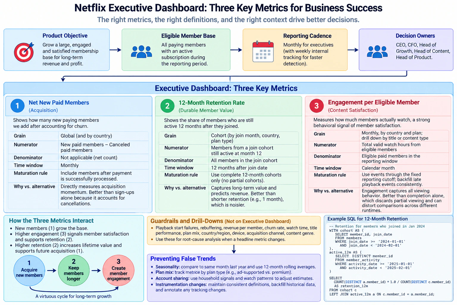
Define the product objective, eligible member base, reporting cadence, and decision owners before selecting exactly three metrics. For each metric, state its grain, numerator, denominator, time window, maturation or censoring rule, and why it represents acquisition, durable member value, content satisfaction, or service quality better than a nearby alternative. Explain how the three metrics interact, what guardrails or drill-downs remain available outside the headline dashboard, and how you would prevent seasonality, plan mix, account sharing, and instrumentation changes from creating false trends.

Short Interview Answer (30-60 seconds)

I would track Net New Paid Members, 12-Month Retention Rate, and Engagement per Eligible Member. Together they cover acquisition, durable member value, and content satisfaction. I would report them monthly with stable eligibility rules, mature cohorts where needed, and separate drill-downs for service quality and false-trend diagnosis.

Detailed Explanation

An executive dashboard should answer three simple questions: Are we growing the paid member base, are members staying, and are members engaging enough to show continued value from the service? I would first define the objective as growing a large, engaged, satisfied paid membership for long-term revenue and profit. The eligible base is paying members with an active subscription during the reporting period. I would use a monthly executive cadence, with weekly internal tracking for faster detection. The decision owners are the CEO, CFO, Head of Growth, Head of Content, and Head of Product.

Useful Questions to Ask the Interviewer
  1. Should the headline dashboard be global only, or should country and plan cuts be visible immediately below each metric?
  2. How should we define an eligible paid member when someone changes plan, pauses, cancels, or rejoins during a reporting period?
  3. Should the executive dashboard remain monthly while weekly internal monitoring is used only for early detection?
  4. Which service-quality measures should remain guardrails rather than become headline metrics?
Which three metrics would you put on a streaming-service executive dashboard? diagram
How to Explain It in an Interview

I would use exactly three headline metrics.

  1. Net New Paid Members — acquisition

This measures whether the paid membership base is growing after cancellations are considered.

  • Grain: Monthly at the global level, with country as an important drill-down.
  • Numerator: New paid members minus canceled paid members during the period.
  • Denominator: Not applicable because this is a net count, not a rate.
  • Time window: One calendar month.
  • Maturation rule: Include a new paid member only after payment has been successfully processed. Apply the same eligibility and cancellation definitions every month.
  • Why this metric: It measures paid acquisition momentum better than sign-ups alone because sign-ups can increase while cancellations offset the gain.

This answers the first executive question: are we adding paying members after accounting for losses?

  1. 12-Month Retention Rate — durable member value

This measures the share of members from a join cohort who are still active twelve months later.

  • Grain: Join-month cohort, with country and plan as drill-downs.
  • Numerator: Members from the join cohort who are still active at month 12.
  • Denominator: All eligible paid members in the original join cohort.
  • Time window: Twelve months after the join date.
  • Maturation rule: Use only cohorts that have completed the full twelve-month observation window. Do not mix partial recent cohorts with fully matured cohorts.
  • Why this metric: It represents durable member value better than short-term retention such as one-month retention, which can be noisy and does not show whether members continue to find value over a longer period.

This metric is delayed. A recent cohort cannot yet have a valid 12-month result, so incomplete cohorts should not be treated as final observations.

  1. Engagement per Eligible Member — content satisfaction

This measures how much eligible members actually watch and provides a behavioral signal of member satisfaction.

  • Grain: Monthly by country and plan, with title or content type available as drill-downs.
  • Numerator: Total valid watch hours from eligible members.
  • Denominator: Eligible paid members in the reporting window.
  • Time window: One calendar month.
  • Maturation rule: Use playback events through a fixed reporting cutoff and backfill late-arriving playback events consistently.
  • Why this metric: Engagement captures all valid viewing behavior. It is a stronger headline measure than completion alone because completion discards partial viewing and can distort comparisons when titles have different runtimes.

The three metrics tell one connected business story. Net new paid members show whether the base is growing. Engagement shows whether members are actively using the service and finding content worth watching. Higher engagement can support retention, while stronger retention increases durable member value and makes future acquisition more valuable. These are relationships to investigate, not automatic proof of causation.

I would keep several guardrails and drill-downs outside the three headline numbers. These include playback start failures, rebuffering, revenue per member, churn rate, watch time, title performance, plan mix, country or region, device, acquisition channel, and content genre. They are diagnostic measures. For example, if engagement falls while playback failures rise, the decline may reflect service quality rather than content demand.

I would also protect the dashboard from false trends. For seasonality, I would compare the same month with the prior year and use a rolling view when useful. For plan mix, I would inspect the metrics by plan so a shift between ad-supported and premium members does not look like a behavioral change. For account sharing, I would use consistent household or usage signals and track changes in those signals over time. For instrumentation changes, I would maintain consistent definitions, validate old and new tracking when possible, backfill historical data when appropriate, and annotate known breaks in the series.

The main limitation is that three executive metrics can summarize business health but cannot explain every movement. Root-cause analysis belongs in the drill-downs. The key validation discipline is to keep the eligible population, formulas, time boundaries, cohort rules, event cutoffs, and instrumentation definitions stable enough that changes in the dashboard represent real business movement rather than measurement changes.

Technical Approach
  1. Define the product objective before choosing any metric: grow a large, engaged, satisfied paid membership that supports long-term revenue and profit.
  2. Define one consistent eligible-member population: paying members with an active subscription during the reporting period.
  3. Set a monthly executive reporting cadence, with weekly internal tracking for faster detection.
  4. Assign the decision owners: CEO, CFO, Head of Growth, Head of Content, and Head of Product.
  5. Choose Net New Paid Members as the acquisition metric.
  6. Choose 12-Month Retention Rate as the durable-value metric and use only fully matured join cohorts.
  7. Choose Engagement per Eligible Member as the content-satisfaction metric using valid watch hours and a fixed reporting cutoff.
  8. Define the grain, numerator, denominator, time window, and maturation rule for every metric.
  9. Keep playback quality, revenue, churn, title, country, plan, device, acquisition-channel, and content-genre measures as guardrails or drill-downs rather than extra headline metrics.
  10. Prevent false trends with seasonality comparisons, plan-level slicing, consistent account-sharing logic, stable instrumentation definitions, appropriate backfills, and annotations for measurement breaks.
Practical Insights

The formulas are simple; the hard part is keeping them trustworthy over time. Net new members can be calculated quickly, but its meaning changes if payment, cancellation, or eligibility rules change. Twelve-month retention is slower because each cohort needs a full year to mature. Engagement depends on reliable playback events and a stable cutoff for late data. More drill-downs help diagnosis but increase data and maintenance work. Weekly internal monitoring gives faster warning, while the monthly executive view stays stable and easy to interpret.

Why Interviewers Ask This

This question tests whether a Data Scientist can turn a complex streaming business into a small set of decision-ready metrics without losing measurement discipline. A strong answer defines the objective, eligible population, grain, numerator, denominator, time window, maturation rules, reporting cadence, and decision owners. It also shows judgment about delayed outcomes, misleading alternatives, seasonality, plan mix, account sharing, instrumentation changes, and the guardrails needed to investigate headline movements.

Common interview mistakes

Common mistakes are putting too many operational measures on the executive dashboard; using sign-ups as acquisition without accounting for cancellations; comparing immature retention cohorts with mature cohorts; using completion alone as the headline satisfaction measure even though it ignores partial viewing and runtime differences; changing the eligible-member definition between periods; treating seasonality or plan-mix shifts as real product changes; ignoring account-sharing effects; interpreting an instrumentation change as a business trend; and assuming that movement between engagement, retention, and acquisition proves causation without drill-down evidence.

Interview tip

Start with the objective, eligible population, cadence, and owners. Then name exactly three metrics. For each metric, give its grain, formula, time window, maturation rule, and nearest alternative. Finish with how the metrics interact and which guardrails you would use to detect false trends.
Interviewer may ask next
How would you handle 12-month retention when the newest member cohorts have not yet had twelve months to mature?

I would exclude incomplete cohorts from the headline 12-month retention result. A cohort should enter that metric only after it has had the full twelve-month observation window. I could monitor shorter-term retention separately as an internal leading indicator, but I would label it as a different metric and would not mix it into the 12-month series. This avoids right-censoring and keeps the numerator and denominator comparable across reporting periods.

What would you do if engagement per eligible member dropped sharply but 12-month retention had not changed?

I would not conclude immediately that durable member value had fallen because retention is a delayed metric. I would drill down engagement by country, plan, title or content type, and device. I would also inspect playback start failures and rebuffering to separate content demand from service-quality problems. Then I would check seasonality, plan-mix shifts, account-sharing changes, late playback events, and instrumentation changes. I would keep the headline metric definition stable and annotate a confirmed measurement break rather than silently changing historical comparisons.

2. How would you evaluate the effectiveness of a 30-day free trial?Model Evaluation And ValidationMediumNetflix

Question Details

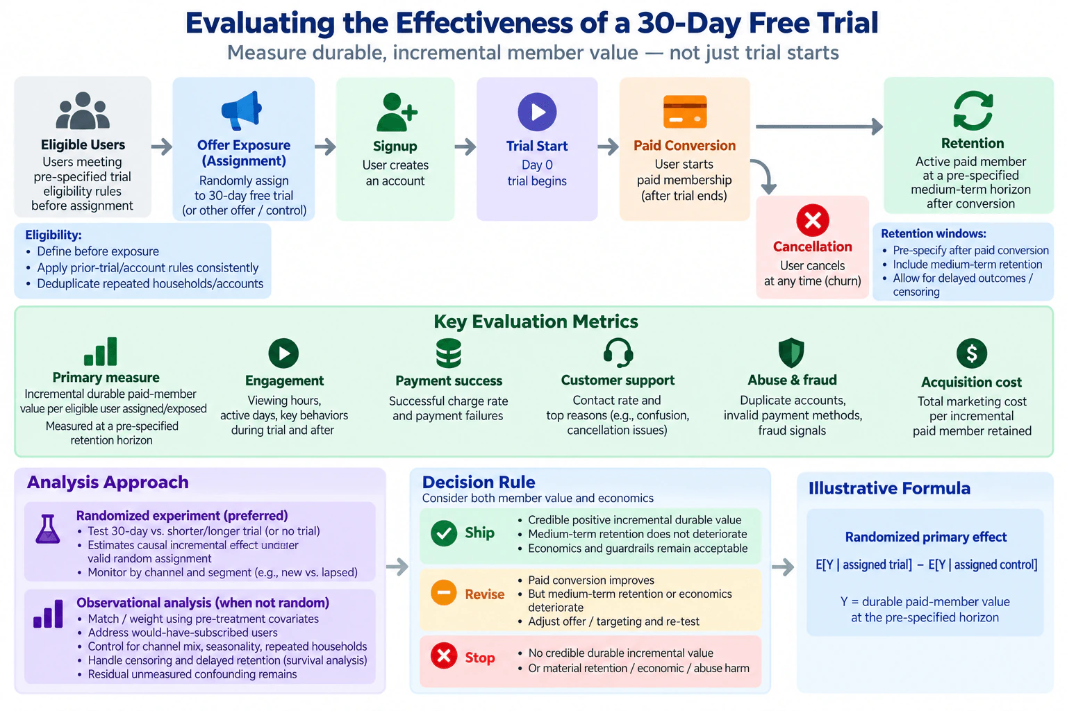
Define eligibility, assignment or offer exposure, signup, trial start, paid conversion, cancellation, and retention windows. Choose a primary measure that reflects durable incremental member value rather than trial starts alone, plus engagement, payment success, customer-support, abuse, and acquisition-cost guardrails. Compare randomized trial-length or offer tests with observational cohort analysis when assignment is not random; address would-have-subscribed users, channel mix, censoring, seasonality, repeated households, and delayed retention. State the ship, revise, or stop rule when conversion improves but medium-term retention or economics deteriorate.

Short Interview Answer (30-60 seconds)

I would measure incremental durable paid-member value per eligible user assigned to the offer, not trial starts alone. I would prefer a randomized trial or offer test, track medium-term retention plus engagement and economic guardrails, and ship only if durable value improves without harming retention or unit economics.

Detailed Explanation

The goal is to learn whether a 30-day free trial creates durable incremental paid-member value, not simply more trial starts or initial conversions. I would define eligibility before exposure, choose a stable assignment unit, and track offer assignment, signup, trial start, paid conversion, cancellation, and a pre-specified medium-term retention outcome. The primary measure should represent durable paid-member value per eligible user assigned or exposed. I would then evaluate engagement, payment success, customer support, abuse, and acquisition cost as guardrails and use the combined evidence for a ship, revise, or stop decision.

Useful Questions to Ask the Interviewer
  1. What exact eligibility and prior-trial rules define the population before offer exposure?
  2. Can users be randomly assigned to the 30-day trial versus no trial or another trial length, or is exposure determined by an existing policy or channel?
  3. What medium-term retention horizon should be pre-specified for the primary outcome, and how long can we wait for delayed outcomes to mature?
  4. Should assignment and deduplication happen at the account, household, or another stable entity level?
  5. Which costs and operational guardrails should be included, especially acquisition cost, payment failures, support burden, and abuse?
How would you evaluate the effectiveness of a 30-day free trial? diagram
How to Explain It in an Interview

First, I would define the analysis population and event sequence before looking at results. Eligible users must satisfy pre-specified trial rules before assignment or exposure. I would then track signup, trial start, paid conversion, and whether a paid member remains active at the pre-specified medium-term horizon or cancels. I would also deduplicate repeated accounts or households using the chosen assignment unit so the same underlying entity does not contaminate multiple comparison groups.

The primary metric should capture durable incremental value. For a randomized test, a clean estimand is E[Y | assigned trial] - E[Y | assigned control], where Y is durable paid-member value at the pre-specified horizon. Using assignment rather than conditioning only on users who actually start or complete the trial keeps the analysis aligned with the randomized design and avoids selecting on post-assignment behavior. Paid conversion is useful, but it is an intermediate outcome rather than sufficient evidence that the trial creates long-term value.

When possible, I would prefer a randomized experiment comparing the 30-day trial with no trial or a shorter or longer offer. Under valid random assignment and consistent treatment implementation, the assignment-based difference estimates the causal incremental effect. I would also examine important pre-specified segments, such as acquisition channel or relevant user cohorts, while avoiding excessive post-hoc slicing that can turn noise into apparent findings.

If assignment is not random, I would use an observational cohort analysis more cautiously. I would compare similar exposed and unexposed users using pre-treatment covariates through matching or weighting. I would explicitly address users who would have subscribed anyway, differences in channel mix, seasonality, and repeated households. These methods can reduce measured confounding, but residual unmeasured confounding may remain, so I would describe the causal evidence as weaker than a randomized experiment.

Retention is delayed, so follow-up time matters. I would pre-specify the medium-term retention horizon after paid conversion and allow enough time for outcomes to mature. Users whose complete retention outcome is not yet observable are censored; I would not silently count them as either retained or churned. If an interim analysis is necessary, a survival-analysis approach can use available follow-up while handling right censoring. I would also compare groups with comparable calendar exposure so seasonality and unequal outcome maturity do not create misleading differences.

Alongside the primary outcome, I would monitor guardrails. Engagement can include viewing hours or active days. Payment success should capture successful charges and payment failures. Customer-support metrics should capture contact rate and important reasons such as confusion or cancellation problems. Abuse checks should look for duplicate accounts, invalid payment methods, or repeated trial behavior. Acquisition cost should be evaluated against the incremental durable value created rather than trial starts alone.

I would report uncertainty around the incremental effect and judge both statistical evidence and practical business significance. I would ship when there is credible positive incremental durable value, medium-term retention does not deteriorate, and economics and guardrails remain acceptable. I would revise when paid conversion improves but medium-term retention or economics deteriorate, for example by changing the offer or targeting and re-testing. I would stop when there is no credible durable incremental value or when retention, economics, abuse, or another important guardrail shows material harm.

Technical Approach
  1. Predefine eligibility before offer exposure, including prior-trial rules and the stable assignment unit.
  2. Deduplicate repeated accounts or households according to that assignment unit.
  3. Track the event sequence consistently: offer assignment or exposure, signup, trial start, paid conversion, cancellation, and the pre-specified retention outcome.
  4. Define the primary measure as durable paid-member value per eligible user assigned or exposed at the pre-specified medium-term horizon.
  5. Randomly assign the 30-day trial versus a control or alternative trial length whenever feasible and estimate the assignment-based incremental effect.
  6. If assignment is observational, match or weight using pre-treatment covariates and address would-have-subscribed users, channel mix, seasonality, and repeated households while acknowledging residual unmeasured confounding.
  7. Handle delayed outcomes and censoring explicitly; use comparable follow-up windows or survival analysis when appropriate.
  8. Evaluate engagement, payment success, customer support, abuse, and acquisition cost as guardrails.
  9. Quantify uncertainty and practical significance for the primary effect and important pre-specified cohorts.
  10. Ship if durable incremental value is credibly positive and guardrails remain acceptable; revise if conversion improves while retention or economics deteriorate; stop if durable value is absent or material harm appears.
Practical Insights

The biggest cost is time. A 30-day trial delays paid conversion, and durable retention requires additional follow-up, so a trustworthy conclusion arrives later than a signup or conversion metric. Randomization gives cleaner causal evidence but requires operational support and enough eligible users. Observational analysis can use existing data, but matching or weighting adds analytical work and cannot remove hidden differences between groups. Household deduplication, channel adjustment, censoring, payment data, support data, abuse signals, and acquisition-cost accounting also increase data and validation effort. More segment analysis can help explain results, but smaller cohorts create wider uncertainty and a greater chance of noisy conclusions.

Why Interviewers Ask This

This question tests whether a candidate can evaluate a product offer causally instead of relying on a simple funnel metric. The interviewer wants to see precise eligibility and event definitions, a durable primary outcome, appropriate randomization when possible, careful observational analysis when assignment is not random, correct handling of censoring and delayed retention, meaningful business guardrails, uncertainty awareness, and disciplined ship, revise, or stop judgment when short-term conversion and medium-term value disagree.

Common interview mistakes

Common mistakes are using trial starts or raw paid conversion as the primary success metric; comparing only users who actually started the trial instead of the assigned population; defining eligibility after seeing results; allowing repeated households or accounts to contaminate groups; treating observational matching as equivalent to randomization; ignoring would-have-subscribed users, channel mix, or seasonality; treating immature retention outcomes as completed outcomes; mishandling censoring; focusing only on statistical significance instead of practical value; and shipping because conversion rises even though medium-term retention, economics, payment success, support burden, or abuse deteriorates.

Interview tip

Lead with the key principle: measure incremental durable member value, not trial starts. Then explain eligibility and assignment, randomized versus observational identification, delayed retention and censoring, the guardrails, and finally the ship, revise, or stop rule. Explicitly discuss the case where conversion improves but retention or economics worsen.

Interviewer may ask next
What would you do if many users have not yet reached the pre-specified medium-term retention horizon when the experiment is reviewed?

I would not label those users as retained or churned prematurely. I would report how much of each group has mature follow-up and confirm that treatment and control have comparable observation opportunities. If possible, I would wait for the pre-specified primary outcome to mature. If an earlier analysis is necessary, I would use a time-to-event method such as survival analysis to handle right censoring and clearly label it as interim evidence. I would not make a final ship decision from paid conversion alone while the durable-value outcome is still materially incomplete.

Suppose paid conversion is clearly higher for the 30-day trial, but medium-term retention is lower and acquisition economics are worse. What would you recommend?

I would not ship based on conversion alone. That pattern means the offer is creating more initial paid conversions without enough durable value. I would choose revise if the opportunity still looks promising: investigate offer length, targeting, channel mix, payment quality, support burden, and abuse, then change the offer or targeting and re-test. If the credible incremental durable-value estimate is not positive, or the retention or economic harm is material, I would stop the offer.

3. What metrics would you prioritize for a multi-task streaming recommender?Model Evaluation And ValidationHardNetflix

Question Details

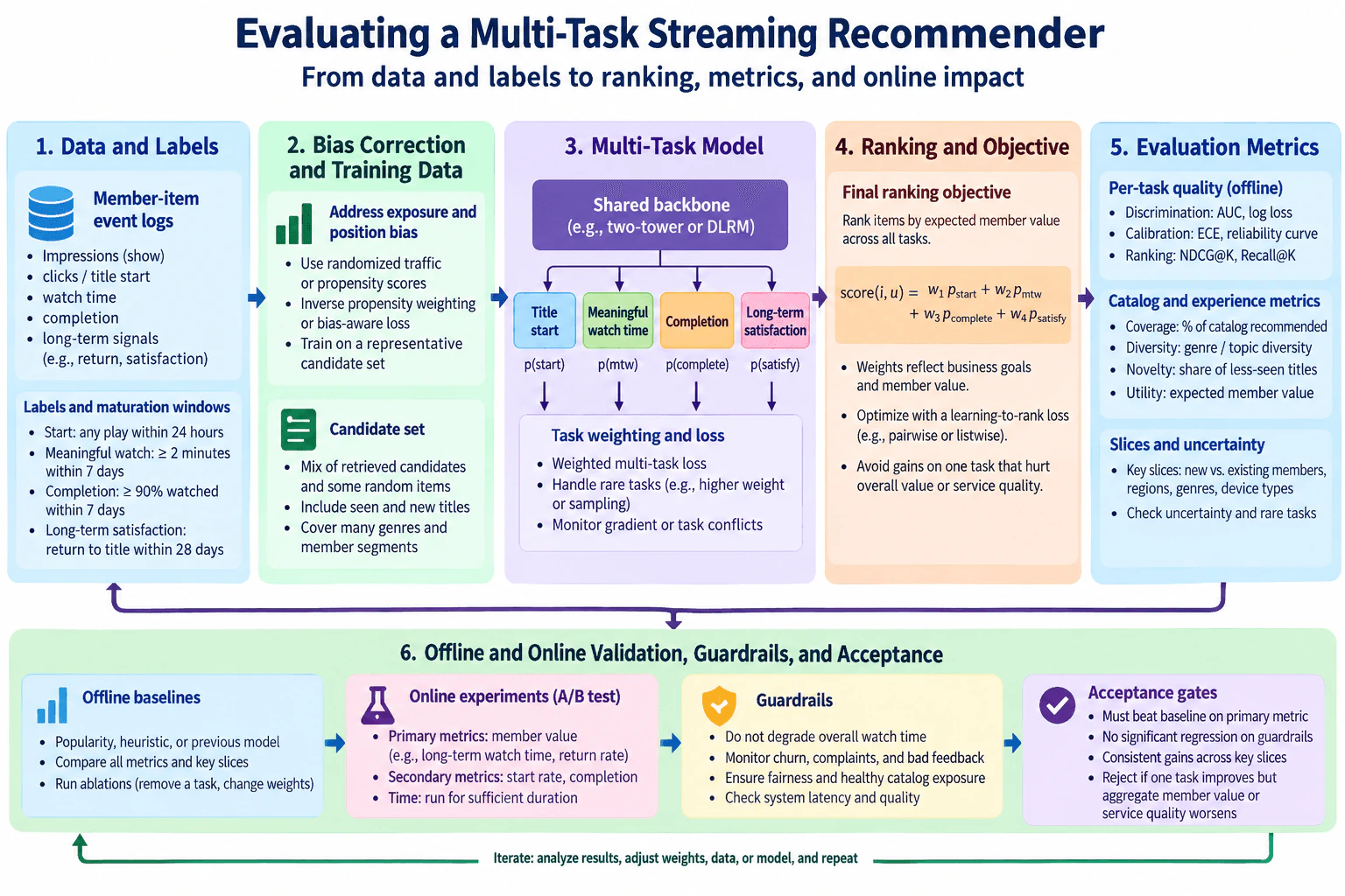
The model jointly predicts several outcomes such as title start, meaningful watch time, completion, and longer-term satisfaction for each member-item opportunity. Define labels, maturation windows, exposure and position bias, task weighting, candidate set, and the final ranking objective. Compare per-task discrimination, calibration, ranking, coverage, diversity, novelty, and utility metrics; inspect gradient or task conflicts, rare tasks, important member and catalog slices, and uncertainty. Specify offline baselines, online experiment metrics, guardrails, acceptance gates, and how a gain on one task can be rejected when aggregate member value or service quality worsens.

Short Interview Answer (30-60 seconds)

I would evaluate each task with discrimination, probability-quality, and calibration metrics, then evaluate the combined ranking with NDCG, Recall, coverage, diversity, novelty, and expected member value. I would also inspect task conflicts, rare tasks, slices, and uncertainty, and ship only after an A/B test improves aggregate value without guardrail regressions.

Detailed Explanation

A multi-task streaming recommender predicts several outcomes for each member-item opportunity: title start, meaningful watch time, completion, and longer-term satisfaction. I would not optimize one task in isolation. I would define each label and its maturation window, correct exposure and position bias, and evaluate every task on a representative candidate set. Then I would evaluate the combined ranking for ranking quality, catalog health, member utility, important slices, rare tasks, task conflicts, and uncertainty. Finally, I would require an online experiment to improve aggregate member value without degrading service-quality guardrails.

Useful Questions to Ask the Interviewer
  1. Which outcome represents the primary member-value goal, and which outcomes are supporting tasks or guardrails?
  2. What candidate set is ranked for each member-item opportunity, and how much randomized traffic is available for estimating exposure or position bias?
  3. How are title start, meaningful watch time, completion, and longer-term satisfaction defined, and when is each label considered mature?
  4. Which member and catalog slices are most important for the launch decision?
  5. Which online metrics and service-quality guardrails are hard acceptance requirements?
What metrics would you prioritize for a multi-task streaming recommender? diagram
How to Explain It in an Interview

Start with the prediction unit. One observation is a member-item opportunity. The multi-task model uses a shared backbone and separate heads for title start, meaningful watch time, completion, and longer-term satisfaction.

Define the labels before choosing metrics. In the approved design, title start means any play within 24 hours. Meaningful watch means at least 2 minutes watched within 7 days. Completion means at least 90% watched within 7 days. Longer-term satisfaction is represented by a return to the title within 28 days. These windows matter because a delayed outcome must not be treated as a negative before its label has had enough time to mature.

Next, address exposure and position bias. The logged data come from titles that members were actually shown, and outcomes are affected by whether an item was exposed and where it appeared. When available, randomized traffic provides cleaner evidence. Propensity scores can also support inverse propensity weighting or another defensible bias-aware loss. The candidate set should be representative rather than limited to the items favored by the current system. The approved design mixes retrieved candidates with some random items, includes seen and new titles, and covers many genres and member segments.

For per-task quality, separate discrimination from probability quality. AUC measures whether positive examples tend to receive higher scores than negative examples. Log loss evaluates probabilistic predictions and penalizes confident wrong predictions. For rare tasks, I would pay special attention to metrics and uncertainty that remain informative under class imbalance rather than relying on simple accuracy.

Calibration is a separate question. A model can rank examples well while producing probabilities that are systematically too high or too low. I would inspect expected calibration error and reliability curves. This matters because the final ranking combines task probabilities, so badly calibrated heads can distort the weighted objective even when their ordering looks reasonable.

For ranking quality, I would prioritize NDCG@K and Recall@K on the final candidate set. NDCG@K rewards putting relevant items near the top of the list. Recall@K measures how much of the relevant set appears in the top K. These metrics evaluate the ordering that the member actually experiences rather than only the quality of an individual prediction head.

The final ranking score combines the task predictions, conceptually as score(i,u) = w1p_start + w2p_mtw + w3p_complete + w4p_satisfy. The weights should reflect member value and product goals, not simply whichever task is easiest to predict. A pairwise or listwise learning-to-rank loss can optimize the combined ordering. I would compare weighting choices and run ablations such as removing one task or changing its weight to understand which signals help the final objective.

Because this is multi-task learning, I would inspect task interactions. Gradients from different task heads can conflict inside the shared model. I would monitor those conflicts and look for cases where improving title start hurts meaningful watch, completion, or satisfaction. Rare tasks also need special treatment because a common task can dominate the weighted loss. Higher weighting or targeted sampling can help, but those choices must be validated against the overall ranking and member-value objective.

Ranking metrics alone are not enough. I would measure catalog coverage, diversity, novelty, and utility. Coverage asks what share of the catalog receives recommendation exposure. Diversity asks whether the ranked list contains a useful mix of genres or topics. Novelty checks whether the system can surface less-seen titles instead of repeatedly showing only familiar items. Utility represents expected member value across the tasks.

I would also break the results down by important slices. The approved design highlights new versus existing members, regions, genres, and device types. I would inspect rare-task performance and uncertainty within important slices because an overall average can hide a serious regression in a smaller population. The launch decision should therefore consider both aggregate results and consistency across key member and catalog segments.

For offline comparison, I would benchmark against a popularity baseline, a simple heuristic, or the previous model. I would compare the full metric set and important slices instead of declaring success from one headline score. I would also run ablations, such as removing a task or changing its weight, to understand the source of any gain or regression.

Offline evidence is only a gate to an online experiment. In the A/B test, the primary metrics should represent member value, such as the long-term watch-time or return-rate examples shown in the approved design. Supporting metrics include title-start rate and completion. The experiment should run for sufficient duration so delayed outcomes can mature and uncertainty can be estimated reliably.

Guardrails determine whether an apparently successful model is still unacceptable. I would reject a model that degrades overall watch time, increases churn, complaints, or bad feedback, creates unhealthy catalog exposure, or worsens system latency or service quality. Statistical significance by itself is not enough. The effect must also be practically useful and must not violate the agreed guardrails.

The acceptance gate is therefore multi-dimensional. The model should beat the baseline on the primary metric, avoid significant guardrail regressions, and show consistent gains across important slices. Most importantly, I would reject a gain on one task if aggregate member value or service quality becomes worse. For example, a higher title-start rate is not a win if it produces weaker meaningful watch, lower completion, worse long-term satisfaction, or degraded service quality.

If the model fails the gate, I would iterate on task weights, data, candidate construction, or model design and repeat the validation cycle. Individual task metrics are diagnostic signals. The final decision is based on the quality of the combined ranking and its measured effect on overall member value under explicit guardrails.

Technical Approach
  1. Define the member-item opportunity and the four task labels with their maturation windows.
  2. Build evaluation data from representative candidate sets and exclude examples whose delayed labels have not matured.
  3. Address exposure and position bias using randomized traffic, propensity-based correction, or another defensible bias-aware method.
  4. Evaluate each task with AUC, log loss, calibration error, and reliability analysis as appropriate.
  5. Evaluate the final ranked list with NDCG@K and Recall@K.
  6. Measure catalog coverage, diversity, novelty, and expected utility.
  7. Inspect rare tasks, gradient or task conflicts, uncertainty, and important member and catalog slices.
  8. Compare against popularity, heuristic, or previous-model baselines and run task-removal or weight-change ablations.
  9. Run an A/B test using aggregate member value as the primary decision signal and task metrics as supporting evidence.
  10. Apply guardrails for overall watch time, churn, complaints, bad feedback, healthy catalog exposure, latency, and service quality.
  11. Ship only when the primary objective improves without unacceptable guardrail or slice regressions; otherwise reject the model and iterate.
Practical Insights

Multi-task evaluation costs more than evaluating one model output because every task has its own label window, metrics, calibration checks, and slice analysis. Ranking metrics also require scoring and ordering candidate sets. Bias correction can increase variance when propensity weights become large, so estimates may become less stable. Rare tasks need enough examples to produce useful uncertainty estimates. More task weights, ablations, and slices increase experiment and maintenance cost. Online tests are slower when long-term labels mature late. The benefit is a safer decision: the system is less likely to ship a model that wins one task while hurting overall member value.

Why Interviewers Ask This

This question tests whether a candidate can evaluate a recommender that predicts several outcomes at once rather than optimizing one convenient metric. The interviewer wants to see whether the candidate can define labels and maturation windows, correct exposure and position bias, evaluate each task separately, assess the final ranking, inspect task conflicts and important slices, quantify uncertainty, connect offline evidence to online experiments, and reject a model when a local task gain harms aggregate member value or service quality.

Common interview mistakes

Common mistakes are optimizing one task as the only success criterion; treating immature delayed labels as negatives; ignoring exposure and position bias; evaluating task heads but not the final ranked candidate set; confusing discrimination with calibration; treating log loss as a ranking metric; tuning weights only for the easiest or largest task; ignoring gradient conflicts and rare tasks; reporting only global averages without important member and catalog slices; treating coverage, diversity, or novelty as substitutes for member utility; trusting offline gains without an A/B test; and shipping because one task improves even when aggregate member value, catalog health, latency, or other guardrails become worse.

Interview tip

Present the answer in layers: labels and bias first, per-task metrics second, final-ranking and catalog metrics third, then slices and uncertainty, and finally the A/B-test guardrails and ship-or-reject gate. Emphasize that a local task gain cannot override aggregate member value.

Interviewer may ask next
How would you handle the fact that longer-term satisfaction matures much later than title-start or watch-time labels?

I would evaluate each task only after its own maturation window has completed. I would not mark a still-pending long-term outcome as a negative. For offline evaluation, I would use examples with enough elapsed time for the required label window or clearly defined task-specific matured subsets. In the online experiment, short-term task metrics can provide early diagnostics, but they cannot replace the final acceptance signal. I would wait for sufficient mature long-term data and report uncertainty before deciding whether the combined recommender improves aggregate member value.

What would you do if title-start AUC and start rate improve, but completion and aggregate member value decline?

I would reject the change even though the start task improved. That pattern suggests the model is over-rewarding items that attract an initial play without creating enough downstream value. I would inspect task weights, calibration, candidate composition, task or gradient conflicts, and affected member or catalog slices. I would run ablations or adjust the multi-task weighting, then repeat offline and online validation. The acceptance rule remains the same: a local gain is not a win when the combined ranking reduces aggregate member value or violates service-quality guardrails.

4. Design a classifier that chooses the best ad-break location in a long video.Machine Learning System DesignEasyNetflix

Question Details

Define the video, scene boundary, candidate timestamp, viewer session, ad opportunity, and interruption-quality labels, including delayed engagement and abandonment outcomes. Design video, audio, subtitle, scene, pacing, historical-viewer, and device features without using information unavailable at playback time; annotation and weak-label generation; baselines and candidate models; temporal and title-held-out validation; calibration and constrained selection. Cover model and feature registry, offline preprocessing, low-latency serving with safe editorial fallback, monitoring, feedback, drift, retraining, privacy, content security, reliability, rollback, and compute cost.

Short Interview Answer (30-60 seconds)

I would score each valid candidate timestamp for interruption quality using only video, audio, subtitle, pacing, viewer, and device information available at playback time. I would calibrate the scores, apply placement constraints, choose the best valid timestamp, and fall back to editorial rules when the model cannot safely serve a result.

Detailed Explanation

The system chooses one candidate timestamp in a long video where inserting an ad should cause the least interruption. The prediction unit is one ad opportunity: a valid candidate timestamp evaluated for the current viewer session. The classifier estimates the probability that an interruption at that point is acceptable. It uses video, audio, subtitle, pacing, viewer, and device features that are available by playback time. The final timestamp is not chosen by the classifier alone: calibrated candidate scores pass through placement constraints, and delayed outcomes such as engagement and abandonment later provide training feedback.

Useful Questions to Ask the Interviewer
  1. Are candidate timestamps limited to detected or editorial scene boundaries, or may the system consider other valid positions?
  2. Which placement constraints are mandatory, such as minimum gaps between ads, avoiding cold opens or endings, and content-policy restrictions?
  3. What playback latency is acceptable, and which media features should therefore be precomputed offline?
  4. Which historical viewer and device attributes are allowed for personalization under the privacy requirements?
  5. Should a low model score, timeout, missing model, or missing feature always fall back to an editorial ad-break rule?
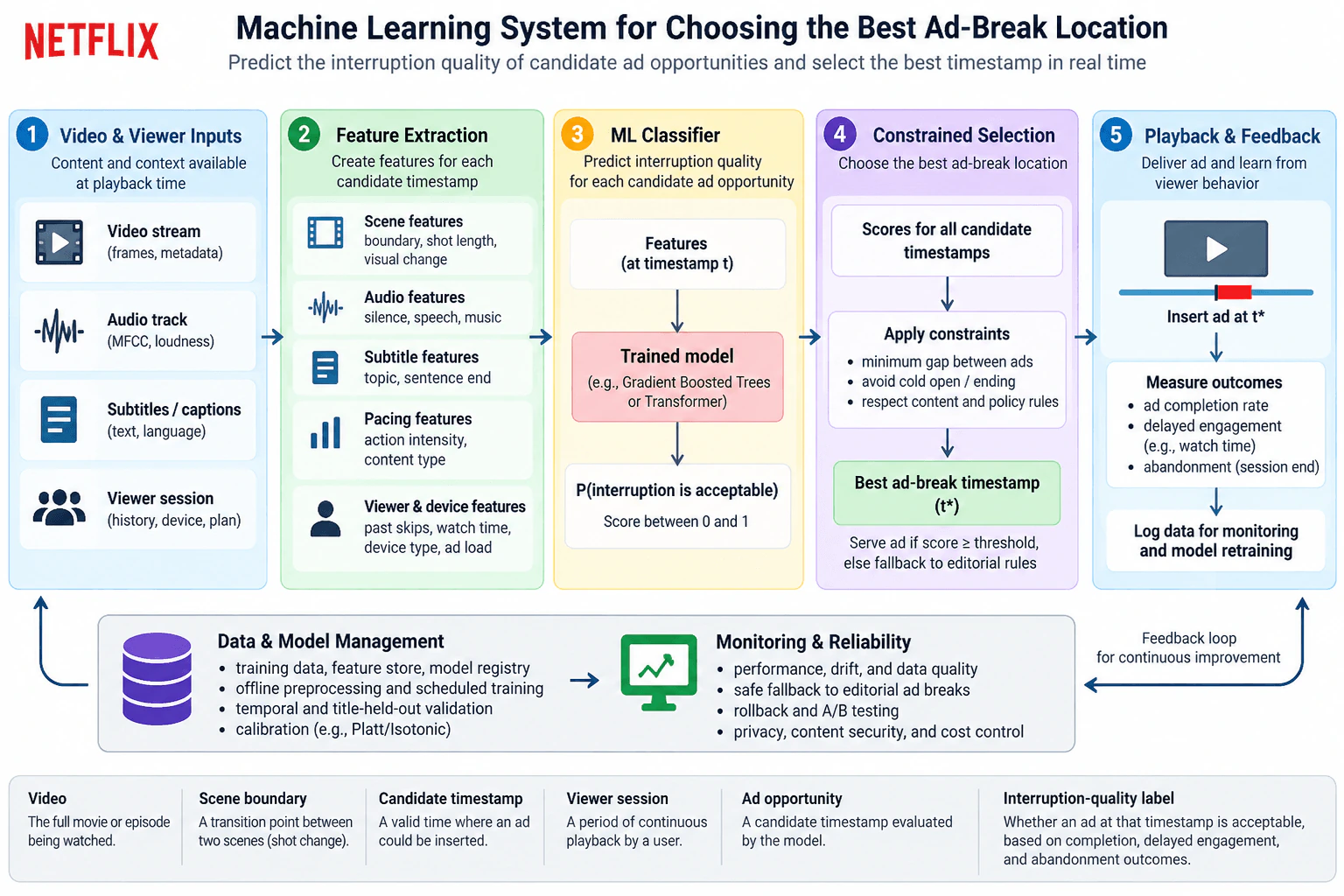
Design a classifier that chooses the best ad-break location in a long video. diagram
How to Explain It in an Interview
1. Define the entities and prediction grain

A video is the full movie or episode being watched. A scene boundary is a transition between scenes or shots. A candidate timestamp is a valid time where an ad could be inserted. A viewer session is a period of continuous playback by a viewer. An ad opportunity is one candidate timestamp evaluated for that viewer session.

For each candidate timestamp t, the classifier estimates P(interruption is acceptable). The score is between 0 and 1. The system later applies constraints and selects the best valid timestamp t*.

2. Build the playback-time inputs

The serving request combines content information and viewer context that are available at playback time. The diagram's inputs are the video stream with frames and metadata, the audio track, subtitles or captions, and viewer-session information such as permitted history, device context, and plan context.

The important rule is time correctness. A feature used to score timestamp t must already exist when that prediction is made. Future watch behavior, future abandonment, or any other later outcome is a label, not a playback-time feature.

3. Extract features for each candidate timestamp

Scene features can include whether the timestamp is near a scene boundary, shot length, and visual change. Audio features can include silence, speech, music, loudness, and other derived audio descriptors. Subtitle features can include topic and whether a sentence is ending. Pacing features can summarize action intensity or content type.

Viewer and device features can include permitted historical skips, watch time, device type, and current ad-load context. Expensive video, audio, subtitle, scene, and pacing features should be precomputed offline when possible. The online path then combines those stored features with current viewer and device context. Using the same registered feature definitions in training and serving reduces training-serving skew.

4. Create interruption-quality labels

Training examples come from historical ad opportunities. The interruption-quality label represents whether placing an ad at that candidate timestamp was acceptable. The diagram uses ad completion, delayed engagement such as later watch time, and abandonment at session end as outcome signals.

Some labels can come from manual annotation. Weak labels can also be derived from observable engagement and abandonment behavior when their meaning is defined clearly. Because engagement and abandonment are delayed, the system must retain the original prediction identity and later join the outcome to the correct video, candidate timestamp, viewer session, and prediction time.

5. Train baselines and candidate models

Start with a simple baseline so there is a reference point. Then compare stronger candidate models. The approved design shows gradient-boosted trees or a Transformer as candidate trained models. Each model receives the features for candidate timestamp t and returns an interruption-quality score.

The offline path contains the training data, feature store, model registry, offline preprocessing, and scheduled training. Version the training data, feature definitions, preprocessing logic, configuration, model artifacts, and evaluation results so every deployed prediction can be traced back to the artifact that produced it.

6. Validate on time and unseen titles

A random split can leak related examples across train and validation data. Use temporal validation so the validation period follows the training period. Also use title-held-out validation so the candidate model is tested on videos not represented in its training partition.

Compare the candidate model against the baseline and do not promote it merely because its training metric improved. The validation gate should check generalization, point-in-time correctness, data quality, calibration, and behavior on relevant slices before the model is registered for serving.

7. Calibrate the classifier score

The constrained selector uses scores and may use a serving threshold, so probability calibration matters. Calibrate the selected classifier on held-out data with a method such as Platt scaling or isotonic calibration, as shown in the diagram. Calibration makes a probability-like score more useful for threshold decisions; it does not replace ranking and validation.

8. Apply constrained selection

The classifier produces scores for all valid candidate timestamps, but it does not independently choose the final break. The selection layer first applies the diagram's constraints: maintain a minimum gap between ads, avoid the cold open and ending, and respect content and policy rules.

Among candidates that remain valid, choose the best ad-break timestamp t*. If the selected candidate satisfies the configured serving threshold, use it. If no candidate safely qualifies, fall back to the editorial ad-break rules.

9. Serve with low latency and safe degradation

At playback time, retrieve the precomputed content features, combine them with current permitted viewer and device features, score the candidate timestamps, and apply the constrained selector. Keep this online path lightweight because playback should not wait for expensive media processing.

Model inference time is only part of end-to-end latency. Feature retrieval, request handling, candidate scoring, constraint evaluation, and response delivery also matter. If the model is missing, the request times out, the service is overloaded, required features are unavailable or stale, or the model otherwise cannot produce a safe decision, use the editorial fallback rather than blocking playback.

10. Measure outcomes and close the feedback loop

After inserting the ad at t*, log the prediction and measure the diagram's outcome signals: ad completion, delayed engagement such as later watch time, and abandonment at session end. Join each delayed outcome back to the original prediction at the correct entity and time.

These joined records become feedback for model-quality monitoring and future training. They should not be treated as features for the prediction that preceded them.

11. Monitor reliability, data, drift, and quality separately

Monitor service health such as latency, errors, timeouts, availability, and fallback usage. Monitor data quality such as missing features, invalid candidate timestamps, stale values, and broken feature contracts. Monitor input and prediction drift separately from model quality. Drift is evidence that data changed; it is not proof that model quality declined.

Also monitor interruption-quality outcomes using the delayed engagement, completion, and abandonment signals. A useful monitoring design therefore separates performance and reliability, data quality, drift, model quality, and viewer or advertising outcomes.

12. Retrain, test, roll back, and control cost

Use the joined feedback in scheduled retraining or when quality evidence justifies retraining. A replacement model must pass the same temporal and title-held-out validation and calibration checks before promotion. The diagram also includes A/B testing as a controlled way to compare an approved candidate with the current serving behavior.

Keep the previous approved model available for rollback. If a new model harms quality or reliability, restore the prior version while the issue is investigated. Protect viewer information and video-derived features with appropriate privacy and content-security controls. Limit access to sensitive data and avoid collecting viewer attributes that are not needed.

Control compute cost by preprocessing expensive media features offline, storing reusable features in the feature store, and scoring only valid candidate timestamps instead of every video frame. The main tradeoff is that richer models and more personalization may improve selection quality, but they can increase latency, privacy risk, compute cost, and operational complexity.

Technical Approach
  1. Define one prediction row as a video, candidate timestamp, and viewer session forming one ad opportunity.
  2. Generate or receive valid candidate timestamps, preferably around scene boundaries and other allowed editorial positions, and remove invalid or duplicate candidates.
  3. Precompute reusable video, audio, subtitle, scene, and pacing features offline and store them with versioned feature definitions.
  4. At playback time, join only features available at or before the decision with permitted viewer and device context.
  5. Build interruption-quality labels from annotation, ad completion, delayed engagement, abandonment, and clearly defined weak-label rules.
  6. Train a baseline and compare candidate models such as gradient-boosted trees and a Transformer.
  7. Validate using temporal and title-held-out splits and reject leakage, point-in-time errors, or poor generalization.
  8. Calibrate the selected model using held-out data, for example with Platt scaling or isotonic calibration.
  9. Register the approved model and its feature and evaluation lineage.
  10. During playback, score all valid candidates and apply minimum-gap, cold-open or ending, and content-policy constraints.
  11. Select the highest acceptable timestamp t* and serve it only when the serving threshold is satisfied.
  12. On timeout, unavailable model, unusable features, overload, or insufficient score, use the editorial fallback.
  13. Log the prediction and later join ad completion, engagement, and abandonment outcomes to the correct prediction.
  14. Monitor service health, data quality, drift, model quality, and outcomes separately.
  15. Retrain from joined feedback, validate and calibrate again, use controlled A/B testing when appropriate, and keep the previous approved model available for rollback.
Practical Complexity & Trade-offs

The expensive work is mainly media preprocessing and model training. Computing video, audio, subtitle, scene, and pacing features offline keeps the playback path faster and cheaper. Online work grows with the number of candidate timestamps because each candidate needs features, a model score, and constraint checks. Restricting evaluation to valid ad opportunities is cheaper than scoring every frame. A Transformer can be more computationally expensive than a simpler tree model, so any quality gain must justify added latency and cost. Calibration adds another offline step but makes threshold decisions more meaningful. Delayed outcomes also slow model-quality feedback because engagement and abandonment are known only later. The editorial fallback improves reliability but may be less personalized than a model-selected break.

Where it is used

This design is useful for long-form video systems that need to place ads at natural interruption points instead of arbitrary times. It also fits any system that scores several pre-approved insertion opportunities using content and session context, applies business or content constraints, and must continue operating safely when machine learning is unavailable.

Why Interviewers Ask This

This question tests whether a candidate can design an end-to-end machine learning system around a time-sensitive ranking decision. The interviewer is looking for correct prediction grain, playback-time feature availability, delayed labels, leakage-safe validation, calibration, constrained selection, low-latency serving, safe fallback behavior, monitoring, feedback, retraining, privacy, reliability, rollback, and compute-cost judgment.

Common interview mistakes

Common mistakes are scoring arbitrary frames instead of valid ad opportunities; using delayed watch time or abandonment as a feature before it exists; allowing information from future playback to leak into training; using random validation that mixes related times or titles; confusing the classifier score with the final constrained timestamp decision; treating an uncalibrated score as a trustworthy probability; using different feature definitions offline and online; failing to join delayed outcomes to the exact original prediction; treating drift by itself as proof that quality fell; monitoring only model metrics while ignoring service health and data quality; blocking playback when the model or features fail; omitting the editorial fallback; and performing expensive media feature extraction in the low-latency serving path when it could be done offline.

Interview tip

Start with the prediction unit and the time boundary. Then walk through inputs, point-in-time features, labels, training, temporal and title-held-out validation, calibration, constrained selection, and playback serving. Finish with fallback, feedback, monitoring, retraining, A/B testing, rollback, privacy, content security, and compute cost. Keep the classifier's probability score separate from the final constraint-based decision.

Interviewer may ask next
How would you prevent delayed engagement and abandonment from leaking into the features used to choose the ad break?

I would separate prediction time from outcome time. The feature vector for candidate timestamp t may contain only information available when that timestamp is scored. Delayed engagement and abandonment occur after the prediction, so they are stored as labels and joined later to the original prediction using the correct video, candidate timestamp, viewer session, and prediction time. Offline training must reproduce this point-in-time boundary. I would also validate feature timestamps and reject any feature whose availability time is later than the prediction time.

What would you do if the Transformer gives better offline quality but makes playback scoring too slow or unreliable?

I would treat end-to-end latency and reliability as deployment constraints, not optimize model quality alone. First I would move expensive media processing to the offline feature path and keep online retrieval and scoring lightweight. Then I would compare the Transformer with the gradient-boosted-tree candidate under the same temporal and title-held-out validation and calibration process. If the Transformer still violates serving requirements, I would choose the simpler eligible model. Regardless of the chosen model, timeout, overload, unavailable model, stale or missing required features, or insufficient serving confidence should route to the editorial fallback, and the previous approved model should remain available for rollback.

5. Design a self-service platform for model deployment and monitoring.Machine Learning System DesignMediumNetflix

Question Details

Design a platform for data scientists to register reproducible training artifacts and deploy approved models without owning infrastructure details. Define dataset, feature, experiment, model, evaluation, deployment, endpoint, batch job, and monitoring records; control-plane APIs; immutable versions; approval gates; environment promotion; online and batch serving; autoscaling; canaries; rollback; and fallbacks. Include lineage, training-serving parity, prediction and delayed-label logging, quality and drift checks, feedback and retraining triggers, tenant isolation, secrets, permissions, auditability, quotas, reliability, disaster recovery, observability, and cost attribution.

Short Interview Answer (30-60 seconds)

I would build a multi-tenant control plane around immutable metadata and model artifacts, then let an orchestrator promote only approved versions into online or batch serving. Canary traffic, autoscaling, rollback, prediction logging, delayed labels, quality and drift checks, retraining triggers, permissions, quotas, audit logs, reliability, and cost attribution make the workflow safe and self-service.

Detailed Explanation

The goal is to let data scientists move approved models into production without managing infrastructure themselves. I would separate the system into a multi-tenant control plane and a serving data plane. The control plane owns versioned metadata, lineage, approvals, environment promotion, deployment configuration, and monitoring configuration. Immutable artifacts contain the code, environment, model files, and configuration needed to reproduce a model version. The data plane supports real-time endpoints and scheduled batch inference. Prediction logs, delayed labels, service telemetry, data checks, drift checks, and model-quality signals close the feedback loop safely while preserving auditability and rollback.

Useful Questions to Ask the Interviewer
  1. Which workloads need real-time endpoints, batch inference, or both?
  2. What approval policy should a model satisfy before promotion from staging to production?
  3. How quickly do delayed labels arrive, and at what entity and prediction time should they be joined back to predictions?
  4. What reliability targets should drive autoscaling, alerting, rollback, and disaster-recovery decisions?
  5. How strict should tenant isolation, quotas, permissions, and cost attribution be across teams or projects?
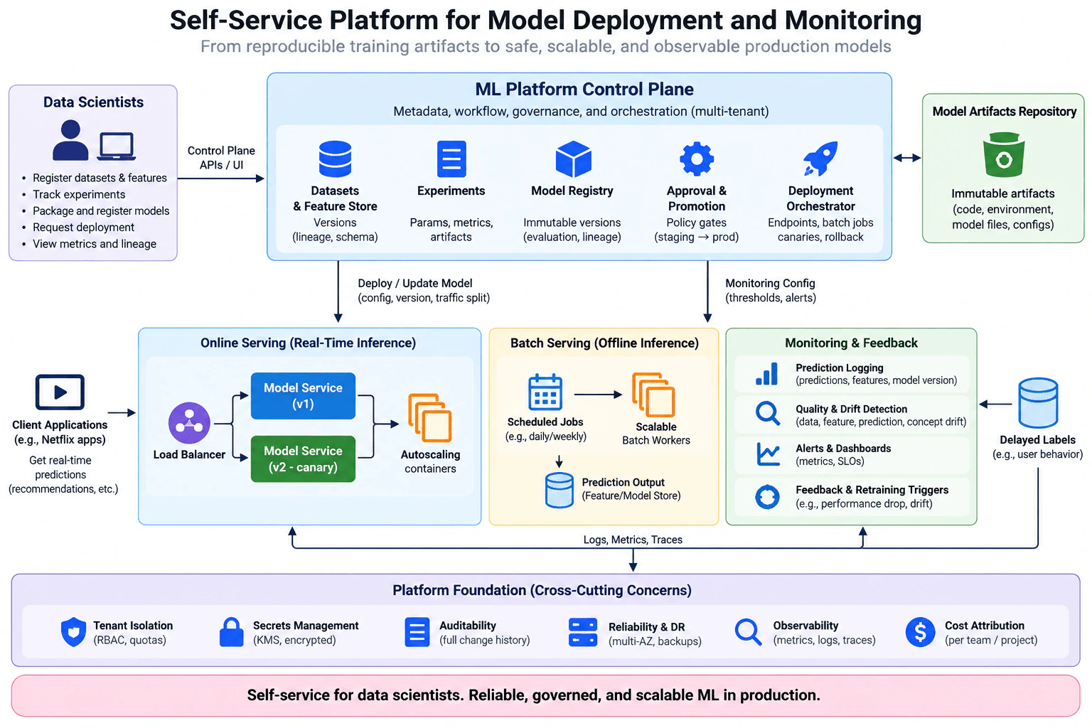
Design a self-service platform for model deployment and monitoring. diagram
How to Explain It in an Interview
1. Start with the platform contract

The platform has two major responsibilities. The control plane stores metadata, applies governance, and orchestrates deployments. The data plane runs inference. A data scientist interacts with the control plane through APIs, an SDK, or a UI rather than directly configuring production infrastructure.

The control plane should expose operations to register and retrieve datasets, features, experiments, models, evaluations, deployments, endpoints, batch jobs, and monitoring configurations. Mutation operations should create new immutable versions rather than silently changing previously approved history.

2. Define the core records

A dataset record identifies a version of input data and keeps its source, schema, and lineage. A feature record identifies a versioned feature definition and its lineage. An experiment record connects parameters, metrics, and produced artifacts. A model record identifies an immutable model version and links it to evaluation evidence and lineage.

An evaluation record stores the evidence used by an approval gate. A deployment record identifies the model version, environment, configuration, traffic policy, and deployment state. An endpoint record represents an online-serving target and records the active model version or versions and traffic assignment. A batch-job record stores the scheduled inference configuration and status. A monitoring record stores the checks, metrics, thresholds, and alerts associated with a deployment.

Together these records form an auditable lineage from dataset and feature versions through experiments, model versions, evaluations, deployments, predictions, and later outcomes.

3. Make reproducibility and lineage immutable

The model artifact repository stores immutable training artifacts such as code, the execution environment, model files, and configuration. The model registry points to these artifacts instead of accepting a mutable file that can change after approval.

Dataset and feature records also use explicit versions. That gives the platform a stable lineage chain: dataset and feature versions lead to an experiment; the experiment produces a model artifact; evaluation evidence is attached to that model version; and a deployment references the approved version.

Training-serving parity comes from keeping feature definitions, schemas, model configuration, and artifact versions explicit and using compatible versioned contracts during serving. This reduces training-serving skew and prevents production from silently interpreting a feature differently from training.

4. Put approval and promotion before deployment

A model should not be deployed merely because its training metric looks good. The model registry links an immutable model version to evaluation evidence. An approval and promotion step applies policy gates before the version can move from staging to production.

The deployment orchestrator accepts an approved model version plus deployment configuration. It creates or updates an endpoint or batch job and records that deployment decision. Because each deployment references immutable versions, the platform can reproduce what was running at a point in time and audit who approved or changed it.

5. Support online and batch serving separately

For online inference, client applications send requests through a load-balancing layer to autoscaled model-service instances. During a canary, most traffic can continue to the current model while a controlled traffic share reaches the candidate version. The deployment record keeps the intended traffic split so promotion or rollback is explicit.

The important latency boundary is end-to-end request latency, not only model execution time. It can include routing, feature access when applicable, queueing, inference, and response handling. No numeric latency target should be invented because the question does not provide one.

For batch inference, scheduled jobs launch scalable workers that run the approved model version over batch inputs and write prediction output. Batch inference is operationally separate from the real-time endpoint even though both consume the same versioned model artifact and configuration contract.

6. Use canaries, rollback, and safe fallback behavior

A new online model version should first receive controlled canary traffic rather than replacing the current production version immediately. The platform observes the candidate while the current version remains available.

If the new deployment becomes unhealthy or violates a promotion condition, the orchestrator can restore traffic to the previously healthy immutable version. This is rollback. The retained healthy version is also a safe platform-level fallback for a missing or failed candidate model. For overload or timeout, the serving tier should apply its configured degradation policy instead of silently returning an unverified prediction. The question does not define the application-specific fallback response, so that behavior should remain configurable rather than invented.

7. Log predictions at the correct grain

Each prediction log needs enough information to identify the request or entity, the features or feature references used for the prediction, the model version, and the prediction itself. This lets the platform connect a later outcome to the exact prediction that preceded it.

Delayed labels arrive after inference, such as later user behavior. They must be joined back to predictions using the correct entity and prediction-time relationship. The system should not simply join to the newest label or newest feature state because that can produce incorrect evaluation and time leakage.

Duplicate, missing, invalid, or late prediction and label events should be handled explicitly so evaluation remains at the intended observation grain.

8. Separate monitoring concerns

Monitoring should not collapse everything into one health score.

Service health covers operational signals such as request failures, latency, saturation, resource usage, and deployment availability. Data-quality checks cover schema violations, missing values, invalid values, and unexpected input behavior. Drift checks compare relevant input, feature, prediction, or concept distributions over time. Drift is evidence that data or relationships changed; it is not by itself proof that model quality declined.

Model quality requires outcomes. When delayed labels arrive and are correctly joined to prediction logs, the platform can evaluate the deployed model using the appropriate evaluation definition. Alerts and dashboards can then distinguish an infrastructure problem from a data problem or a model-performance problem.

9. Close the feedback and retraining loop carefully

Monitoring can create a retraining trigger when a configured condition is met, such as a label-based quality decline or a drift condition that the team has chosen to act on. A trigger should start a new experiment or training workflow; it should not directly overwrite the production model.

The resulting model becomes a new immutable version. It must be registered, evaluated, approved, promoted, and canaried through the same control-plane path as any other model. This prevents automated retraining from bypassing validation and governance.

10. Build multi-tenancy into the platform foundation

Tenant isolation should separate teams or projects in metadata, serving resources, permissions, and quotas. Role-based permissions determine who can register artifacts, approve a model, promote to an environment, or alter a deployment. Quotas protect shared infrastructure from one tenant consuming all available capacity.

Secrets should be managed by a dedicated secrets or key-management mechanism rather than embedded in model artifacts or deployment configuration. Auditability means recording control-plane actions and changes so the platform can reconstruct who changed what and when.

Cost attribution should associate serving, batch, storage, and supporting-resource consumption with the responsible team or project. This makes self-service sustainable because users can understand the operational cost of their deployments.

11. Design for reliability and disaster recovery

Critical control-plane and serving components should be deployed redundantly, while recoverable metadata and configuration should have durable backups and a disaster-recovery process. The diagram represents this as multi-availability-zone operation and backups without claiming a numeric recovery objective that the question does not provide.

Online serving also needs autoscaling so capacity can respond to demand. A missing or failed candidate model should not leave the platform unable to serve when the previously healthy immutable version can be restored. Monitoring must cover both platform health and individual model deployments.

12. Make observability part of every layer

Logs, metrics, and traces should connect control-plane deployment activity, serving behavior, and monitoring results. A deployment should be traceable from its model version and configuration to runtime health and prediction logs. This supports incident analysis, rollback decisions, debugging, capacity planning, and cost attribution.

The final design is a self-service control plane over immutable metadata and model artifacts, connected to separate online and batch serving paths. Approval gates and environment promotion control what reaches production. Canary deployment and rollback reduce release risk. Prediction and delayed-label logging create a trustworthy feedback loop. Monitoring separates service health, data quality, drift, and model quality, while tenant isolation, secrets, permissions, quotas, auditability, reliability, disaster recovery, observability, and cost attribution make the platform practical to operate.

Technical Approach
  1. Define the self-service contract: data scientists register versioned artifacts and request deployment through control-plane APIs, an SDK, or a UI.
  2. Create immutable records for dataset, feature, experiment, model, evaluation, deployment, endpoint, batch job, and monitoring configuration, with lineage between them.
  3. Store immutable code, environment, model files, and configuration in the model artifact repository and reference them from the registry.
  4. Require evaluation evidence and an approval gate before environment promotion.
  5. Let a deployment orchestrator create or update online endpoints and batch jobs using an approved model version and configuration.
  6. For online serving, route through a load balancer to autoscaled model services and use controlled canary traffic before full promotion.
  7. Keep the previous healthy immutable model version available so the orchestrator can roll back a failed deployment or use it as a safe model-level fallback.
  8. Run batch inference independently through scheduled jobs and scalable workers while preserving the same model-version contract.
  9. Log predictions with the request or entity, features or feature references, model version, and prediction; later join delayed labels at the correct entity and prediction time.
  10. Monitor service health, data quality, drift, and label-based model quality separately and expose configured alerts and dashboards.
  11. Let qualifying monitoring conditions trigger a new experiment or retraining workflow, but require the resulting model to pass registration, evaluation, approval, promotion, and canary deployment again.
  12. Apply tenant isolation, secrets management, permissions, quotas, audit logs, reliability, backups, observability, and per-team or per-project cost attribution across the platform.
Time & Space Complexity

The main cost is operational complexity rather than one algorithmic Big-O term. Immutable versions and lineage use more metadata and artifact storage, but they make deployments reproducible and rollback reliable. Canary deployments temporarily run more than one model version and therefore consume extra serving capacity, but they reduce release risk. Autoscaling controls capacity as demand changes, although aggressive scaling can increase cost while conservative scaling can increase queueing or failures. Prediction logging and delayed-label storage add data volume and join work, but they are necessary for trustworthy production evaluation. Multi-tenant isolation, permissions, quotas, audit logs, backups, and disaster recovery add platform work, yet they prevent self-service from becoming unsafe. The largest maintenance burden is keeping metadata, serving configuration, monitoring, and lineage contracts consistent as the platform evolves.

Where it is used

This design is useful when many data-science teams need a common path from trained models to production. It fits organizations that support both low-latency application inference and scheduled batch scoring, require approvals before production changes, want reproducible model versions and lineage, need controlled canary releases and rollback, or must evaluate deployed models after labels arrive later. It is especially useful when platform engineers want to hide infrastructure details while still enforcing tenant isolation, permissions, quotas, auditability, reliability, observability, and cost ownership.

Why Interviewers Ask This

This question tests whether a candidate can connect reproducible ML development with safe production operations. The interviewer wants to see a clear separation between control-plane metadata and orchestration and data-plane inference, immutable lineage and approval before deployment, correct handling of online and batch serving, canary and rollback strategies, prediction and delayed-label feedback, distinct service, data, drift, and model-quality monitoring, and practical platform concerns such as permissions, quotas, tenant isolation, secrets, reliability, disaster recovery, observability, and cost attribution.

Common interview mistakes

Common mistakes are building only a model-serving endpoint and ignoring the control plane; letting model artifacts or feature definitions change after approval; deploying from a training metric without separate evaluation evidence and an approval gate; mixing online and batch execution into one path; calling a traffic split a canary without retaining a safe rollback version; monitoring only CPU, latency, or drift while ignoring data quality and delayed-label model quality; treating drift as proof that model quality declined; logging predictions without the model version or correct entity and time information needed to join delayed labels; allowing automated retraining to bypass evaluation and approval; hiding secrets inside artifacts; forgetting tenant permissions and quotas; and designing self-service without audit logs, disaster recovery, observability, or cost attribution.

Interview tip

Draw the control plane first, then the online and batch data-plane paths, and finally the monitoring feedback loop. State explicitly that versions are immutable, approval precedes promotion, canaries retain a rollback target, and drift is separate from delayed-label model quality. Finish with the cross-cutting platform controls rather than turning them into separate architectures.

Interviewer may ask next
How would you handle delayed labels without evaluating the wrong prediction or introducing time leakage?

I would give each prediction a stable identifier or an equivalent entity-and-prediction-time key and log the model version, prediction, and features or feature references used at inference time. When the outcome arrives later, the feedback process joins it to the prediction that existed before that outcome was known. It should not use the newest feature state or simply attach a label to the latest prediction. Duplicate, missing, late, or invalid events should be detected explicitly. Model-quality calculations then operate only on correctly matched prediction-outcome pairs. This preserves the observation grain and avoids look-ahead leakage.

What would you do if a canary version becomes unhealthy during a traffic spike while the platform is close to its quota?

I would first route traffic away from the unhealthy canary and restore the previously healthy immutable version through the deployment orchestrator. Autoscaling can add capacity only within the tenant's configured quota, so the serving layer should not assume unlimited resources. If demand still exceeds safe capacity, the endpoint should apply its configured overload or timeout policy rather than silently returning an unverified prediction. The platform should record the rollback, service metrics, traces, quota pressure, and cost impact. The failed candidate remains an immutable version for diagnosis, and any corrected model must pass evaluation, approval, promotion, and canary deployment again.

6. Design a scalable system for custom image ads using style transfer and diffusion models.Machine Learning System DesignHardNetflix

Question Details

Advertisers provide approved source assets and creative constraints, and the system generates policy-compliant image variants. Define request, asset, prompt, brand-style, output, review, and conversion-label contracts. Design licensed-data ingestion, conditioning and fine-tuning or adapter training, style and identity controls, safety and brand validators, human approval, immutable model-prompt-policy registry, asynchronous generation, GPU scheduling, caching and deduplication, rollout and rollback, quality and business evaluation, feedback and retraining, drift and abuse monitoring, copyright and privacy controls, tenant isolation, secret handling, reliability, auditability, and generation and review cost.

Short Interview Answer (30-60 seconds)

I would use an asynchronous pipeline from approved assets and constraints to brand-conditioned diffusion generation, automated safety and brand validation, human approval, and ad delivery. GPU scheduling, caching, deduplication, immutable model-prompt-policy lineage, tenant-isolated storage, monitoring, and conversion feedback make the system scalable, auditable, measurable, and safe to roll back.

Detailed Explanation

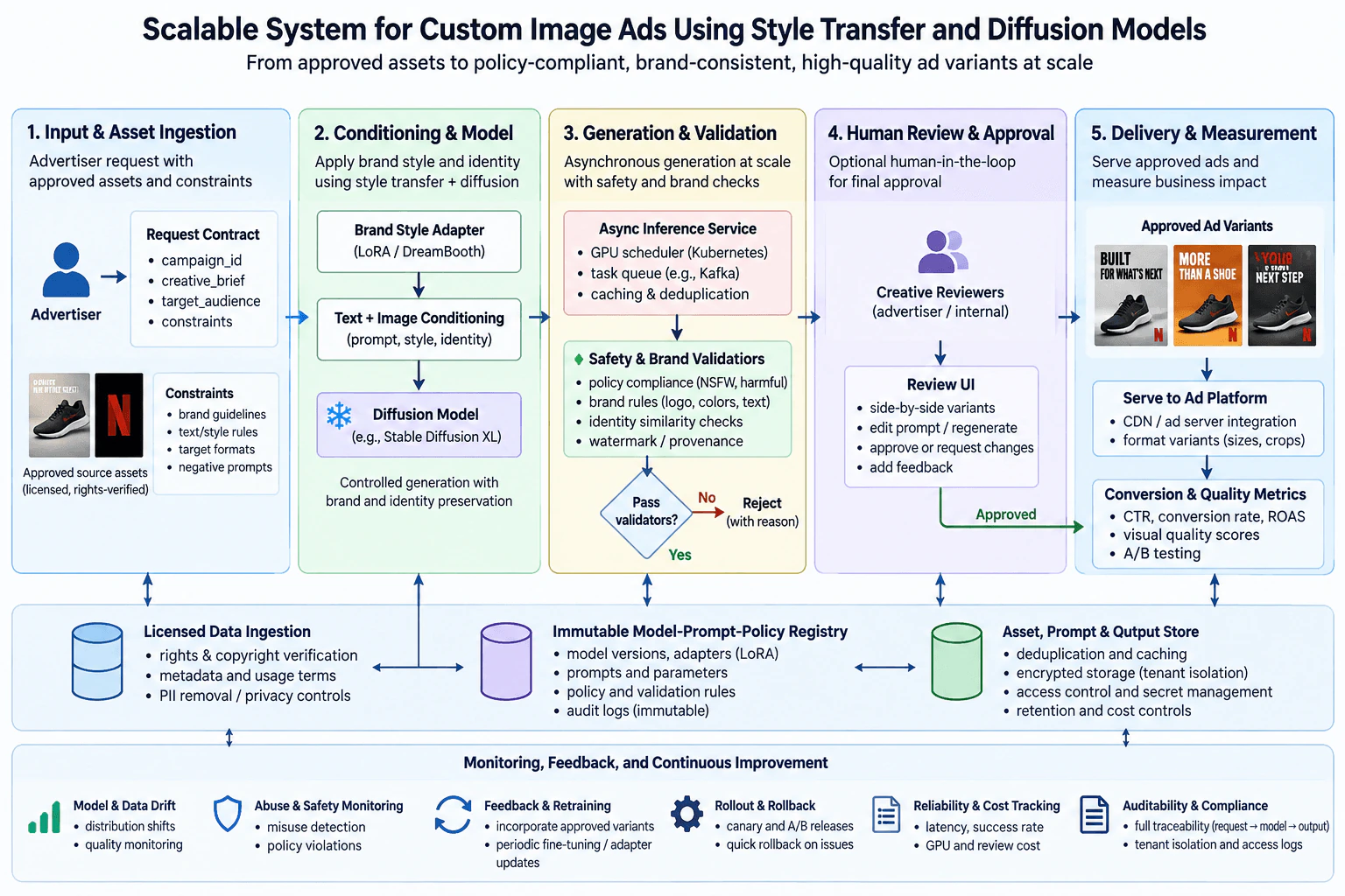
The goal is to generate multiple custom image-ad variants from approved advertiser assets while preserving brand identity and enforcing policy. I would separate offline model or adapter preparation from asynchronous generation and from final ad serving. The main online workflow is: ingest a request and approved assets, apply text-and-image conditioning plus brand-style controls, generate variants on scheduled GPU workers, validate them, send passing variants to human review, serve only approved outputs, and join later quality and conversion outcomes back to the exact generated image. Immutable lineage connects every request, model, prompt, policy, output, review, and outcome.

Useful Questions to Ask the Interviewer
  1. Are all advertiser assets already licensed and rights-verified, or should ingestion enforce those checks?
  2. Is human approval mandatory for every generated variant, or only for selected risk tiers?
  3. Which brand constraints are hard rules, such as logos, colors, text, style, and identity preservation?
  4. Is generation always asynchronous, or is there any interactive generation-latency requirement?
  5. Which business labels should be recorded for each served output: impressions, clicks, conversions, or return on ad spend?
  6. What tenant-isolation, retention, privacy, and deletion rules apply to assets, prompts, generated images, adapters, and logs?
  7. What limits should control the number of generated variants and human-review cost per request?
Design a scalable system for custom image ads using style transfer and diffusion models. diagram
How to Explain It in an Interview
1. Define the contracts first

I would begin with explicit contracts because they make the rest of the system reproducible and auditable.

The request contract contains the campaign identifier, creative brief, target audience, and creative constraints. The asset contract contains the approved source images, logos, license metadata, usage rights, and tenant ownership. The prompt contract contains the prompt template or text, generation parameters, and prompt version. The brand-style contract contains brand guidelines such as colors, logo rules, text rules, style constraints, and identity requirements.

The output contract identifies each generated image and links it to the request, source assets, prompt, model or adapter version, policy version, and generation parameters. The review contract records approval, rejection, requested changes, reviewer feedback, and review status. The conversion-label contract links impressions, clicks, conversions, and related business outcomes to the exact served output.

The grain matters. One campaign can generate many image variants, so delayed outcomes should join back to the exact output that was served rather than only to the campaign.

2. Ingest only approved and rights-verified assets

The first stage is Input & Asset Ingestion. Advertisers provide approved source assets and creative constraints. Licensed Data Ingestion verifies rights and copyright metadata, usage terms, and privacy requirements before an asset can be used for generation or model adaptation.

The Asset, Prompt & Output Store keeps source assets, prompts, generated images, and metadata in encrypted tenant-isolated storage. Access control and secret management prevent one advertiser from reading another advertiser's private assets or model artifacts. Retention and deletion policies apply to stored creative data and logs according to the product's requirements.

Invalid, missing, duplicated, expired, or unauthorized assets should be rejected before GPU work begins.

3. Separate offline adaptation from generation

Offline preparation can train or update a Brand Style Adapter using licensed data when stronger brand specialization is required. The diagram represents this as a brand-style adapter using LoRA or DreamBooth-style adaptation. The resulting artifact must be versioned and registered before it is used by generation.

That offline adaptation path is separate from asynchronous inference. A generation request should not start a new training run automatically. Instead, it resolves an already approved model and adapter version from the registry.

For many requests, text-and-image conditioning may be sufficient. Adapter training adds customization but also adds GPU cost, storage, evaluation, maintenance, and overfitting risk. I would use the lightest mechanism that meets the brand requirement.

4. Apply text, image, style, and identity conditioning

The Conditioning & Model stage combines the approved source assets with the prompt, brand style, and identity controls. The diffusion model then generates candidate images. The diagram uses Stable Diffusion XL as an example of the diffusion-model layer, but the architecture should depend on the registered model contract rather than hard-coding one implementation.

The conditioning layer should preserve all generation-affecting inputs and versions so the same output can be explained later. If a prompt, source image, adapter, model version, or policy version changes, that becomes a distinct generation configuration.

5. Generate asynchronously on scheduled GPU workers

Generation is computationally expensive, so I would use an Async Inference Service rather than place diffusion inference in the ad-serving request path. A task queue, such as Kafka in the diagram, buffers generation jobs. A GPU scheduler, represented by Kubernetes in the diagram, assigns work to available GPU workers.

This design absorbs bursts and lets the system apply tenant quotas, backpressure, autoscaling, retries, and admission control. End-to-end generation latency includes queue time, GPU scheduling, model execution, validation, storage, and review. Model execution time is only one part of that latency.

If the queue is overloaded, the safe behavior is to delay or reject new generation work according to policy. The system should never skip safety validation or serve an unapproved result just to improve availability.

6. Use caching and deduplication before wasting GPU cycles

Equivalent generation requests can be expensive duplicates. I would compute a deduplication key from all inputs that materially affect generation: source-asset versions, prompt and parameters, brand constraints, model version, adapter version, and other deterministic configuration.

If an equivalent eligible result already exists, the system can reuse it instead of launching another GPU job. If the same logical job is already running, a retry should attach to that job rather than create duplicate work.

The cache must never ignore model, prompt, asset, adapter, or policy versions. An incomplete cache key could return an image created under the wrong creative or safety configuration.

7. Store immutable generation lineage

The Immutable Model-Prompt-Policy Registry records model versions, adapters, prompt versions and parameters, policy rules, validation rules, and audit history. Generated outputs reference those immutable versions.

The Asset, Prompt & Output Store keeps the corresponding source and result artifacts. Together, these two stores make the request-to-output path reproducible: request -> assets -> prompt -> model or adapter -> policy -> generated output -> review -> served output.

This lineage is necessary for audits, incident investigation, copyright review, privacy requests, evaluation, retraining, and rollback.

8. Validate safety and brand compliance before review

Every generated candidate enters Safety & Brand Validators before it can progress. The automated validators check policy compliance, harmful or disallowed content, brand rules such as logos, colors, and text, identity similarity when required, and watermark or provenance requirements when those controls are part of the product policy.

The validation result is a decision gate. If a candidate fails, it follows the reject path and the system records the reason. If it passes, it can continue to human review.

Passing automated validation does not mean the image is guaranteed to be good. It means it passed the configured automated gates. Creative quality and business value still require separate evaluation.

9. Use human review as the final approval step when required

The Human Review & Approval stage presents passing variants to creative reviewers. Reviewers can compare variants side by side, edit the prompt or request regeneration, approve an image, request changes, and add feedback.

Only approved variants become eligible for serving. Rejected, failed, or pending-review images remain ineligible.

Human review improves control but introduces latency and cost. Automated validation should therefore remove obvious failures before a person spends time reviewing them. Review time and review cost should be measured separately from GPU generation cost.

10. Serve only approved stored images

After approval, the system sends the Approved Ad Variants to the serving integration. The diagram shows a Serve to Ad Platform step with CDN or ad-server integration and format variants such as different sizes and crops.

The diffusion model is not called in the ad-serving request path. Serving should read a prepared approved asset from storage or a delivery layer. That keeps delivery predictable and isolates expensive generation from serving latency.

If generation fails or no new variant is approved, the safe fallback is to keep using an existing approved creative or produce no new variant. The system should not weaken validation rules to maintain throughput.

11. Evaluate quality and business outcomes separately

The Delivery & Measurement stage tracks quality and business evidence for approved variants. The diagram includes click-through rate, conversion rate, return on ad spend, visual-quality scores, and A/B testing.

These signals answer different questions. Visual-quality scores describe image characteristics. Human review captures creative acceptability. Policy validators capture safety and compliance. Conversion metrics describe business performance. Service metrics describe system reliability.

A release should not be approved only because the training objective or one visual-quality metric improved. It should satisfy the relevant safety, brand, review, operational, and business gates.

12. Join delayed outcomes to the exact output

Business outcomes arrive after the generation event, sometimes much later. The feedback pipeline must join impressions, clicks, conversions, and other labels to the exact served output identifier and its lineage.

That prevents a common mistake where all variants in the same campaign receive the same outcome label. Correct joins preserve the relationship between the generated creative and the result observed after serving.

The joined data can support evaluation, controlled experiments, and future retraining, but only when the underlying assets and labels are permitted for that use.

13. Feed approved evidence into retraining

The Monitoring, Feedback, and Continuous Improvement path can incorporate approved variants and reviewer feedback into future model or adapter updates. Retraining should be a controlled offline process rather than an automatic direct reaction to every conversion.

Training examples must be rights-cleared, privacy-compliant, deduplicated, versioned, and linked to the original output and outcome. Candidate model or adapter versions should pass offline quality checks, safety and brand validation, and controlled release gates before promotion.

This prevents noisy or abused feedback from immediately changing production behavior.

14. Monitor health, drift, abuse, quality, and outcomes independently

The diagram separates several monitoring concerns.

Model & Data Drift monitors distribution shifts and quality trends. Drift is a warning signal, not proof of a quality regression. Abuse & Safety Monitoring detects misuse attempts and policy violations. Reliability & Cost Tracking measures latency, success rate, GPU consumption, and review cost. Auditability & Compliance preserves request-to-model-to-output traceability, tenant isolation, and access logs.

I would also monitor queue depth, GPU utilization, retry rate, generation failures, validation rejection rate, review backlog, storage failures, and serving availability where appropriate.

15. Roll out and roll back model changes safely

New model versions, adapters, prompt templates, and policy configurations should use controlled rollout. The diagram calls out canary and A/B releases followed by quick rollback when issues appear.

The registry makes rollback practical because the system knows the exact previous model, adapter, prompt, and policy configuration. If a new version causes safety failures, quality regression, reliability issues, or unacceptable cost, new generation traffic can be routed back to the last approved configuration.

Rollback changes future generation behavior. Existing generated images keep their immutable historical lineage so the system can still explain which configuration produced them.

16. Treat privacy, tenant isolation, secrets, reliability, and cost as cross-cutting concerns

Copyright and privacy controls begin at Licensed Data Ingestion and continue through storage, training, generation, review, and logs. Tenant isolation applies to source assets, prompts, outputs, caches, adapters, access controls, and audit history. Secrets belong in controlled secret management rather than prompts or image metadata.

Reliability controls include asynchronous queues, idempotent retries, deduplication, backpressure, autoscaling, failure recording, and safe degradation. Auditability requires immutable model-prompt-policy records and request-to-output traceability.

Cost has at least two major components in this design: GPU generation cost and human-review cost. GPU cost grows with the number of generated variants, regeneration attempts, model size, and adaptation work. Human cost grows with the number of variants sent for review and the complexity of each decision. Caching, deduplication, quotas, careful variant counts, and automated rejection before human review reduce unnecessary work.

Final decision

The final architecture is a five-stage governed pipeline: Input & Asset Ingestion -> Conditioning & Model -> Generation & Validation -> Human Review & Approval -> Delivery & Measurement. Licensed Data Ingestion, the Immutable Model-Prompt-Policy Registry, and the Asset, Prompt & Output Store support that main flow. Monitoring, feedback, retraining, rollout and rollback, reliability, cost tracking, tenant isolation, and auditability operate across the system. The central rule is simple: generate asynchronously at scale, but allow only validated and approved images to cross the serving boundary.

Technical Approach
  1. Validate the request contract, approved source assets, rights metadata, creative constraints, and tenant identity.
  2. Store versioned asset, prompt, brand-style, request, output, review, and conversion-label records.
  3. Resolve the approved diffusion model, brand-style adapter if required, generation parameters, and policy version from the immutable registry.
  4. Build a deduplication key from every generation-affecting input and reuse an eligible cached result when available.
  5. Otherwise enqueue the generation job in the asynchronous inference pipeline.
  6. Schedule the job onto GPU workers under capacity limits, tenant quotas, retry rules, and backpressure.
  7. Apply text-and-image conditioning, brand style, and identity controls to the diffusion model and generate candidate variants.
  8. Store each candidate and its complete request-to-model-to-output lineage.
  9. Run safety, brand, identity, and applicable provenance or watermark validators.
  10. Reject failed candidates with recorded reasons; route passing candidates to human review when required.
  11. Allow reviewers to approve, request changes, regenerate, and attach feedback.
  12. Serve only approved stored variants through the ad-delivery path and required format transformations.
  13. Join delayed impressions, clicks, conversions, visual-quality signals, and review outcomes to the exact served output.
  14. Monitor drift, abuse, policy violations, latency, success rate, queue health, GPU cost, review cost, tenant isolation, and audit logs.
  15. Use rights-cleared approved examples and feedback for controlled offline retraining or adapter updates.
  16. Evaluate candidate versions, use canary or A/B rollout, and roll back future generation to the last approved configuration when release gates fail.
Time & Space Complexity

GPU generation is the largest compute cost, so expense increases with the number of requests, number of variants per request, regeneration attempts, model size, and adaptation work. Caching and deduplication can save substantial GPU work, but the cache key must include all generation-affecting versions and parameters. Asynchronous queues improve scalability but add queue waiting time and require backpressure, retries, idempotency, and failure handling. Human review adds another cost and can become a throughput bottleneck, so automated validators should reject obvious failures first. Stronger brand adaptation can improve consistency but adds training, storage, evaluation, and rollback complexity. More variants may improve creative choice but also increase GPU, storage, validation, and review cost. Immutable lineage and tenant isolation add metadata and operational overhead, but they are necessary for reproducibility, privacy, audits, and safe rollback.

Where it is used

This design is useful for creative-generation systems that must produce many advertiser-specific image variants from approved source assets while maintaining safety, brand consistency, reproducibility, and business measurement. It fits workflows such as creating alternate product-ad layouts, adapting an approved creative to several placements, generating brand-consistent campaign variants, and testing approved images against conversion outcomes. It is especially appropriate when generation is expensive enough to run asynchronously and when copyright, privacy, human approval, tenant isolation, and auditability are first-class requirements.

Why Interviewers Ask This

This question tests whether the candidate can design the complete production system around generative models rather than describing only diffusion inference. The interviewer is looking for clear data contracts, licensed-data handling, model conditioning and adaptation, scalable GPU execution, safety and brand validation, human approval, immutable lineage, reliable serving, tenant isolation, privacy, monitoring, business evaluation, feedback, retraining, rollout, rollback, and cost judgment. It also tests whether the candidate can separate generation quality, policy compliance, operational health, and business performance.

Common interview mistakes

Common mistakes are focusing only on the diffusion model; accepting unlicensed or cross-tenant assets; failing to define request, asset, prompt, brand-style, output, review, and conversion-label contracts; mixing offline adapter training with online generation; placing diffusion inference in the ad-serving request path; using an incomplete cache key; allowing duplicate retries to launch duplicate GPU jobs; skipping backpressure during overload; treating an automated validator pass as proof of creative quality; serving rejected or pending-review images; losing the request-to-model-to-output lineage; joining conversions only at campaign level instead of to the exact served output; retraining from feedback without checking rights and privacy; treating drift as proof that quality declined; promoting a new model from one offline metric; ignoring rollback; storing tenant assets or secrets without isolation; and accounting for GPU cost while ignoring human-review cost.

Interview tip

Present the answer as the same five stages shown in the diagram: Input & Asset Ingestion, Conditioning & Model, Generation & Validation, Human Review & Approval, and Delivery & Measurement. Then explain the registry, storage, and monitoring layer underneath. Emphasize that generation is asynchronous, only validated and approved images reach serving, and every output keeps immutable lineage for feedback, audits, rollout, rollback, and cost control.

Interviewer may ask next
How would you prevent duplicate generation jobs while making sure cached outputs are still correct?

I would give each logical generation request an idempotency identity and compute a deduplication key from every input that can change the result: source-asset versions, prompt and generation parameters, brand constraints, model version, adapter version, and relevant configuration. If the same job is already running, a retry attaches to the existing job instead of launching another GPU task. If an equivalent eligible result is already stored, it can be reused. Any material input change creates a different key. The system must also check approval and policy state, because a previously rejected or unapproved output must never become a reusable serving result just because its generation inputs match.

What would you do if a new model version improves visual quality but increases safety failures, GPU cost, or human-review time?

I would not promote it based on visual quality alone. The current approved version remains the rollback target. I would evaluate the new version separately on safety and brand validation, reviewer approval and review time, generation reliability, GPU cost, visual quality, and business outcomes. Then I would use a limited canary or A/B rollout. A safety or policy regression should stop the rollout immediately. If the problem is cost or review burden, I would compare the extra quality or business value with the additional expense before expanding traffic. Because the model, adapter, prompt, and policy versions are immutable in the registry, the system can identify exactly which configuration produced each output and route future generation back to the last approved version if necessary.

7. Write SQL for a three-day weighted moving average of product sales.Data EngineeringEasyNetflix

Question Details

Using standard SQL over sales(date DATE, product_id INTEGER, sales_volume INTEGER), where there is at most one row per product-date and dates do not skip within a product, return date, product_id, and weighted_avg_sales. For each product, compute 0.5 * current_day + 0.3 * previous_day + 0.2 * day_before_previous, and return only dates having both preceding rows. Preserve numeric precision, order by product and date, and explain how LAG establishes the required grain. Define whether null sales rows are rejected or treated as missing before the calculation, and ensure one product cannot affect another.

Short Interview Answer (30-60 seconds)

I would calculate two LAG values for each product, ordered by date, inside a CTE. Then I would compute 0.5 times current sales plus 0.3 times the previous value plus 0.2 times the value before that, keeping only complete three-day windows.

Detailed Explanation

See the Code while reading this explanation.

The task is to calculate a new sales number for each product using three consecutive days. The current day counts the most, the day before counts a little less, and the day before that counts the least. Each product must be handled separately so its sales never mix with another product. The first two usable days for a product cannot produce an answer because two earlier days are not available. We also need a clear rule for missing sales values and must keep any decimal part in the final result.

Useful Questions to Ask the Interviewer
  1. Should a row with NULL sales_volume be rejected, or should it be treated as missing before the calculation?
  2. Can I rely on the stated contract that there is at most one row per product-date and dates do not skip within a product?
  3. Should weighted_avg_sales keep decimal precision without rounding to an integer?
Write SQL for a three-day weighted moving average of product sales. diagram
How to Explain It in an Interview

The input contract is sales(date DATE, product_id INTEGER, sales_volume INTEGER), with at most one row per product-date. Therefore, the required grain is one row for one product on one date.

For this solution, NULL sales_volume rows are treated as missing and filtered out before LAG is calculated. This matches the approved diagram's explicit null policy.

Next, I calculate LAG(sales_volume, 1) and LAG(sales_volume, 2). LAG reads earlier rows while keeping the current product-date row. PARTITION BY product_id creates an independent window for each product, so sales from one product can never affect another. ORDER BY date establishes chronological order inside each product.

I calculate the LAG values in a CTE named lagged. This is important because the outer query can then filter on the calculated previous values. The outer WHERE keeps only rows where both prev_1 and prev_2 exist, which removes incomplete three-row windows.

The weighted calculation is 0.5 * sales_volume + 0.3 * prev_1 + 0.2 * prev_2. The weights sum to 1.0, so no additional division is needed. Decimal coefficients preserve fractional results when necessary.

Finally, ORDER BY product_id, date returns the results grouped by product and in date order. For example, for product 1 with sales 100, 120, and 90, the third day's value is 0.5 * 90 + 0.3 * 120 + 0.2 * 100 = 101.0.

Technical Approach
  1. Start from sales at the stated one-row-per-product-date grain.
  2. Apply the chosen null policy by removing rows where sales_volume IS NULL before the window calculation.
  3. In a CTE, calculate LAG(sales_volume, 1) and LAG(sales_volume, 2) with PARTITION BY product_id ORDER BY date.
  4. In the outer query, calculate 0.5 * current sales + 0.3 * prev_1 + 0.2 * prev_2.
  5. Keep only rows where both lag values are present.
  6. Return date, product_id, and weighted_avg_sales ordered by product_id and date.
Practical Insights

The database must process the sales rows in date order within each product. If the required order is not already available from the execution plan, a sort may be needed, commonly making the ordering work about O(n log n) for n rows. The window calculation itself scans the ordered rows. The query avoids a self-join and keeps the logic simple. Maintenance depends mainly on preserving the one-row-per-product-date contract and the stated date-order assumptions.

Code
WITH
  lagged AS (
    SELECT
      date,
      product_id,
      sales_volume,
      -- Read the immediately preceding usable sales value within this product.
      -- PARTITION BY prevents data from another product from entering the window.
      LAG (sales_volume, 1) OVER (
        PARTITION BY
          product_id
        ORDER BY
          date
      ) AS prev_1,
      -- Read the usable sales value two positions earlier in the same product.
      -- ORDER BY date gives LAG the required chronological row order.
      LAG (sales_volume, 2) OVER (
        PARTITION BY
          product_id
        ORDER BY
          date
      ) AS prev_2
    FROM
      sales
      -- Chosen null policy: treat NULL sales as missing and remove them
      -- before building the per-product LAG window.
    WHERE
      sales_volume IS NOT NULL
  )
SELECT
  date,
  product_id,
  -- Decimal coefficients preserve fractional precision in the result.
  -- The weights sum to 1.0, so no additional division is required.
  0.5 * sales_volume + 0.3 * prev_1 + 0.2 * prev_2 AS weighted_avg_sales
FROM
  lagged
  -- Return only complete three-row windows with both preceding values present.
WHERE
  prev_1 IS NOT NULL
  AND prev_2 IS NOT NULL
  -- Produce deterministic presentation order by product and then date.
ORDER BY
  product_id,
  date;
Why Interviewers Ask This

This question tests whether the candidate can use SQL window functions correctly, preserve the one-row-per-product-date grain, isolate calculations by product, handle incomplete three-day windows and null sales explicitly, preserve numeric precision, and return deterministic ordered output.

Common interview mistakes

Common mistakes are forgetting PARTITION BY product_id and mixing products, omitting ORDER BY date inside LAG, trying to filter LAG expressions directly in the same query block's WHERE clause, returning the first two rows even though their three-row history is incomplete, losing decimal precision, leaving NULL handling undefined, or using a self-join when LAG expresses the required relationship more directly.

Interview tip

Start by stating the grain: one row per product-date. Then explain PARTITION BY product_id, ORDER BY date, the two LAG values, the outer filtering step, and the explicit NULL policy. Finish by checking one weighted calculation aloud.

Interviewer may ask next
Why do we use PARTITION BY product_id in both LAG expressions?

PARTITION BY product_id creates a separate ordered window for every product. Each LAG therefore reads only earlier rows belonging to the same product. Without the partition, a row could use a previous value from another product, which would make the weighted result incorrect.

What changes if sales_volume can be NULL?

The missing-value policy must be defined before calculating the window. In this solution, NULL sales_volume rows are treated as missing and filtered out before LAG is calculated, exactly as shown in the final diagram. If the business instead requires every calendar date to remain part of the three-day window, filtering out a NULL row would change the meaning of the preceding rows, so a different policy such as rejecting the data or explicitly filling the missing day's value would need to be agreed first.

8. Write SQL for daily active users and first-purchase conversion over seven days.Data EngineeringMediumNetflix

Question Details

Assume today is 2025-09-01. Use users(user_id, signup_date), events(user_id, event_date, event_type), and orders(order_id, user_id, order_date, amount) to return one row for each date from 2025-08-26 through 2025-09-01. For each date, calculate dau as distinct users with at least one event, new_buyers as users whose first-ever order date is that date, and conversion_rate = new_buyers / dau, rounded to two decimals with a zero-safe denominator. Count duplicate events once per user-day, count each buyer once, preserve dates with zero activity through a calendar spine, and prevent event-order joins from multiplying users or amounts.

Short Interview Answer (30-60 seconds)

Build a seven-day calendar spine, deduplicate events by user and date, aggregate DAU, find each user's first-ever order, aggregate new buyers by first-order date, and join both aggregates by date. Use COALESCE and NULLIF so a zero-DAU day returns a 0.00 conversion rate.

Detailed Explanation

See the Code while reading this explanation.

The task is to produce seven daily rows, from August 26 through September 1. For each day, show how many different people used the service, how many people made their first purchase ever on that day, and the ratio between those two counts. Repeated use by the same person on one day should count once. A day must still appear even when nobody used the service. The two counts should be worked out separately so combining activity and purchase records does not accidentally count people more than once.

Useful Questions to Ask the Interviewer
  1. Can I assume event_date and order_date are already normalized to the same business date and time zone?
  2. Should a day with dau = 0 return conversion_rate = 0.00 rather than NULL?
  3. Can I use PostgreSQL-style generate_series for the calendar spine?
Write SQL for daily active users and first-purchase conversion over seven days. diagram
How to Explain It in an Interview

I would start by stating the final grain: one row per calendar date. The four logical stages should match the diagram: build the seven-date calendar, compute daily DAU, find first-ever buyers, and combine the daily aggregates.

First, create a calendar spine containing exactly 2025-08-26 through 2025-09-01. This guarantees seven rows even when a date has no events or no first purchases.

Second, deduplicate events to one (user_id, event_date) row. This prevents multiple events from the same user on the same day from inflating DAU. Then group by event_date and count those user-day rows.

Third, find each user's first-ever purchase by calculating MIN(order_date) across the available order history. Do not filter orders to the seven-day reporting window before finding the minimum, because an earlier historical order would mean a later order is not the user's first purchase. After that, group the first-order dates to calculate new_buyers per day. Each buyer contributes at most once.

The question defines new_buyers independently as users whose first-ever order date equals that reporting date. It does not require those buyers to also have an event on that same date. I would follow that definition exactly rather than introducing an extra event-membership condition.

Finally, left join the already-aggregated DAU and new-buyer datasets to the calendar spine by date. Do not join raw events directly to raw orders, because that can create many-to-many row multiplication and inflate counts or amounts. Replace missing counts with zero. For the rate, calculate new_buyers / dau, cast the numerator to a numeric type, use NULLIF to protect against division by zero, round to two decimals, and use an outer COALESCE so a zero-DAU day returns 0.00.

The diagram uses PostgreSQL-style syntax because it shows generate_series and ::numeric. The main tradeoff is that the true first-ever-order calculation may need to examine substantial order history. In a large production system, an already-maintained first-purchase table or indexed historical aggregate could reduce repeated work, but the logical result must remain the same.

Technical Approach
  1. Generate the seven required dates from 2025-08-26 through 2025-09-01.
  2. Deduplicate events to one row per (user_id, event_date).
  3. Group those rows by date to calculate DAU.
  4. Calculate MIN(order_date) per user over the available order history to find each first-ever order.
  5. Group those first-order dates to calculate new_buyers by date.
  6. Left join daily DAU and daily new buyers to the calendar spine.
  7. Replace missing counts with zero.
  8. Calculate conversion_rate = new_buyers / dau, protect against zero DAU, and round to two decimals.
  9. Order the seven final rows by date.
Practical Insights

The event side reads the reporting-window events, removes duplicate user-day activity, and groups the remaining rows by date. The order side can be more expensive because finding a true first-ever purchase may require historical orders for every relevant buyer. After aggregation, the intermediate results are tiny because they contain only daily rows. Operationally, calculating the two metrics independently makes the query easier to test and prevents silent double counting from a detailed event-to-order join.

Code
-- PostgreSQL-style SQL is assumed because the audited diagram uses generate_series and numeric casting.
WITH
  dates AS (
    -- Calendar spine defines the final grain and guarantees all seven requested dates.
    SELECT
      CAST(d AS date) AS dt
    FROM
      generate_series (
        DATE '2025-08-26',
        DATE '2025-09-01',
        INTERVAL '1 day'
      ) AS g (d)
  ),
  active_user_days AS (
    -- Deduplicate to one row per user-day so repeated events do not inflate DAU.
    SELECT DISTINCT
      user_id,
      event_date
    FROM
      events
    WHERE
      event_date BETWEEN DATE '2025-08-26' AND DATE  '2025-09-01'
  ),
  daily_dau AS (
    -- Each remaining user-day contributes exactly one active user to its date.
    SELECT
      event_date AS dt,
      COUNT(*) AS dau
    FROM
      active_user_days
    GROUP BY
      event_date
  ),
  first_orders AS (
    -- Use full available order history so the minimum is truly the user's first-ever order.
    SELECT
      user_id,
      MIN(order_date) AS first_order_date
    FROM
      orders
    GROUP BY
      user_id
  ),
  daily_new_buyers AS (
    -- Each user appears once in first_orders, so each buyer is counted once on the first-order date.
    SELECT
      first_order_date AS dt,
      COUNT(*) AS new_buyers
    FROM
      first_orders
    WHERE
      first_order_date BETWEEN DATE '2025-08-26' AND DATE  '2025-09-01'
    GROUP BY
      first_order_date
  )
SELECT
  d.dt AS date,
  -- Missing daily aggregates mean zero activity or zero first buyers on that date.
  COALESCE(a.dau, 0) AS dau,
  COALESCE(b.new_buyers, 0) AS new_buyers,
  -- NULLIF prevents division by zero; outer COALESCE makes zero-DAU dates return 0.00.
  COALESCE(
    ROUND(
      CAST(COALESCE(b.new_buyers, 0) AS numeric) / NULLIF(COALESCE(a.dau, 0), 0),
      2
    ),
    0.00
  ) AS conversion_rate
FROM
  dates AS d
  -- Join only pre-aggregated daily metrics, never raw events directly to raw orders.
  LEFT JOIN daily_dau AS a ON a.dt = d.dt
  LEFT JOIN daily_new_buyers AS b ON b.dt = d.dt
  -- Deterministic ordering makes the seven-day output easy to validate.
ORDER BY
  d.dt;
Why Interviewers Ask This

This tests whether the candidate can preserve the correct grain while combining activity and purchase data. The interviewer is looking for correct distinct-user counting, true first-ever purchase logic, a calendar spine for missing dates, safe division, and protection against row multiplication from joining detailed event and order records before aggregation.

Common interview mistakes

Common mistakes are joining raw events directly to raw orders, which can multiply rows; using raw event counts instead of one user-day per person; finding the minimum order only inside the seven-day window, which can incorrectly classify an existing buyer as new; counting multiple orders from one buyer; starting from the events table and dropping zero-activity dates; dividing by zero; requiring new buyers to also be active that day even though the question does not say that; and calculating a seven-day post-activity purchase window instead of counting users whose first-ever order date is exactly the reporting date.

Interview tip

State the grain first: one row per date. Then explain the four diagram stages in order and emphasize that DAU and first buyers are aggregated independently before the final date join. Calling out the raw event-order row-multiplication risk shows that you understand data correctness, not just SQL syntax.

Interviewer may ask next
How would you change the query if event_date and order_date were timestamps instead of already-normalized dates?

Define the business time zone first, convert both timestamps consistently to that zone, and derive the business date before deduplication or aggregation. DAU should still use one (user_id, business_date) row. The true first purchase should be determined from the earliest order timestamp before converting that timestamp to its business date for daily counting. Then join the daily aggregates to the same seven-date calendar spine.

Why should the first-order calculation use full order history instead of filtering orders to the seven reporting dates first?

Because new_buyers means users whose first-ever order occurs on that date. If a user purchased before 2025-08-26 and purchases again during the reporting window, filtering first would hide the older purchase and incorrectly classify the later order as the user's first. Compute the earliest order over available history first, then filter those first-order dates to the seven-day reporting window.

9. Write SQL to select the highest-scoring eligible friend candidate for user 3.NEWData EngineeringHardNetflix

Question Details

Use users(user_id,name), friends(user_id,friend_id), likes(user_id,page_id), and blocks(user_id,blocked_id). For John, whose user_id is 3, exclude John, existing friends, and anyone John has blocked. Give each candidate 3 points per distinct mutual friend and 2 points per distinct page liked by both John and the candidate. Return exactly potential_friend_name and friendship_points for the top candidate, with a deterministic user-ID tie-break. Treat friendship direction consistently, deduplicate repeated edges and likes before counting, avoid multiplying mutual-friend and shared-like rows when combining signals, and return no row when no eligible candidate exists. In the reported sample, Alice scores 2 and is selected.

Short Interview Answer (30-60 seconds)

Normalize and deduplicate friendships, deduplicate likes, filter to eligible users, aggregate mutual-friend and shared-like points separately, then add the scores. Rank by friendship_points descending and user_id ascending. In the reported sample, Alice is selected with 2 points.

Detailed Explanation

See the Code while reading this explanation.

The task is to choose the best new person for John to connect with. John cannot be chosen himself, and people who are already connected to him or whom he has blocked are not allowed. A candidate earns points from friends they share with John and from pages they both like. Repeated relationship or like records must not give extra credit. The two kinds of points are counted separately and then added. Ties are broken using the smaller user ID. If nobody is allowed, the result should contain no row.

Useful Questions to Ask the Interviewer
  1. Should friendship be treated as undirected even if only one direction is stored in the friends table?
  2. Should the blocking rule exclude only users John has blocked, as stated, or also users who have blocked John?
  3. Which SQL dialect should I use? I will use PostgreSQL to match the approved diagram.
Write SQL to select the highest-scoring eligible friend candidate for user 3. diagram
How to Explain It in an Interview

First, I establish the grain of each relationship. Grain means what one row represents. For friendships, I normalize each pair with LEAST(user_id, friend_id) and GREATEST(user_id, friend_id). DISTINCT then makes repeated edges or reverse duplicates represent only one friendship. I expand each normalized friendship into both directions so every user's friend list can be queried consistently.

For likes, I keep one distinct row per (user_id, page_id). This prevents repeated like rows from increasing the score.

Next, I build the eligible candidate set from users. I exclude user 3, anyone already connected to user 3, and anyone for whom blocks.user_id = 3 and blocks.blocked_id equals that candidate. The question only says to exclude people John has blocked, so I do not add a reverse-block rule.

Then I calculate the two scoring signals independently. Each distinct mutual friend contributes 3 points. Each distinct page liked by both John and the candidate contributes 2 points. The two signals are grouped separately to one row per candidate before they are joined. This prevents a candidate's mutual-friend rows from multiplying their shared-like rows.

Finally, I LEFT JOIN both aggregated score sets back to every eligible candidate. COALESCE converts a missing signal to zero, so an eligible candidate with no mutual friends or shared likes can still remain with 0 points. I add the two values, order by friendship_points DESC and user_id ASC, and use LIMIT 1. The user_id ordering makes ties deterministic. If the eligible set is empty, the final SELECT naturally returns no row.

The final output contains exactly potential_friend_name and friendship_points. user_id is used internally only for filtering and deterministic tie-breaking. In the reported sample, Alice has 2 points and is selected.

Technical Approach
  1. Normalize each friendship into a canonical unordered pair and remove repeated or self-referential edges.
  2. Expand each canonical friendship into both directions for consistent friend lookup.
  3. Deduplicate likes to one row per user and page.
  4. Build eligible candidates by excluding user 3, John's existing friends, and users John blocked.
  5. Compute 3 points per distinct mutual friend in a separate grouped result.
  6. Compute 2 points per distinct shared liked page in another separate grouped result.
  7. LEFT JOIN both score sets to eligible candidates and use zero for missing signals.
  8. Add the two scores, order by friendship_points descending and user_id ascending, and return the first row.
  9. Project exactly potential_friend_name and friendship_points.
Practical Insights

The main cost comes from deduplicating friendship and like records, finding John's relationships, grouping the two scoring signals, and joining those aggregated results to the eligible candidates. The query may need extra memory for DISTINCT and GROUP BY operations. Keeping each scoring signal at one row per candidate before combining them also makes the logic easier to maintain and avoids inflated results caused by many-to-many row multiplication.

Code
WITH
  friend_edges AS (
    -- Canonicalize each undirected friendship and remove reverse or repeated duplicates.
    SELECT DISTINCT
      LEAST (user_id, friend_id) AS a,
      GREATEST (user_id, friend_id) AS b
    FROM
      friends
      -- Ignore self-edges because they are not valid friendships for this scoring rule.
    WHERE
      user_id <> friend_id
  ),
  all_friends AS (
    -- Expand every canonical edge in both directions for consistent friend lookup.
    SELECT
      a AS user_id,
      b AS friend_id
    FROM
      friend_edges
    UNION ALL
    SELECT
      b AS user_id,
      a AS friend_id
    FROM
      friend_edges
  ),
  john_friends AS (
    -- Keep John's existing friends at one friend_id per row.
    SELECT
      friend_id
    FROM
      all_friends
    WHERE
      user_id = 3
  ),
  dedup_likes AS (
    -- Keep one row per user and page so duplicate likes cannot add extra points.
    SELECT DISTINCT
      user_id,
      page_id
    FROM
      likes
  ),
  eligible AS (
    -- Build the allowed candidate set before calculating any scoring signal.
    SELECT
      u.user_id,
      u.name
    FROM
      users u
    WHERE
      u.user_id <> 3
      -- Exclude anyone who is already John's friend after friendship normalization.
      AND NOT EXISTS (
        SELECT
          1
        FROM
          john_friends jf
        WHERE
          jf.friend_id = u.user_id
      )
      -- Exclude users John has blocked, exactly as required by the question.
      AND NOT EXISTS (
        SELECT
          1
        FROM
          blocks b
        WHERE
          b.user_id = 3
          AND b.blocked_id = u.user_id
      )
  ),
  mutual_scores AS (
    -- Aggregate mutual-friend points independently to one row per candidate.
    SELECT
      e.user_id,
      3 * COUNT(DISTINCT cf.friend_id) AS mutual_points
    FROM
      eligible e
      JOIN all_friends cf ON cf.user_id = e.user_id
      JOIN john_friends jf ON jf.friend_id = cf.friend_id
    GROUP BY
      e.user_id
  ),
  like_scores AS (
    -- Aggregate shared-like points separately to prevent signal row multiplication.
    SELECT
      e.user_id,
      2 * COUNT(DISTINCT cl.page_id) AS like_points
    FROM
      eligible e
      JOIN dedup_likes cl ON cl.user_id = e.user_id
      JOIN dedup_likes jl ON jl.user_id = 3
      AND jl.page_id = cl.page_id
    GROUP BY
      e.user_id
  )
  -- Start from all eligible candidates so zero-signal candidates are not dropped.
SELECT
  e.name AS potential_friend_name,
  COALESCE(m.mutual_points, 0) + COALESCE(l.like_points, 0) AS friendship_points
FROM
  eligible e
  LEFT JOIN mutual_scores m ON m.user_id = e.user_id
  LEFT JOIN like_scores l ON l.user_id = e.user_id
  -- Rank by score first and user_id second so ties always resolve deterministically.
ORDER BY
  friendship_points DESC,
  e.user_id ASC
  -- If eligible is empty, this returns no row; otherwise it returns exactly the top candidate.
LIMIT
  1;
Why Interviewers Ask This

This question tests whether you can translate business rules into correct SQL while controlling data grain. It checks your handling of duplicate relationship data, undirected friendships, eligibility filtering, independent aggregation of multiple one-to-many signals, prevention of join multiplication, zero-score candidates, deterministic tie-breaking, and an exact output contract.

Common interview mistakes

Common mistakes are treating friendship direction inconsistently, counting duplicate friendship edges or likes more than once, forgetting to exclude John or his existing friends, applying a reverse blocking rule that the question did not request, joining raw mutual-friend rows directly to raw shared-like rows and multiplying counts, using an INNER JOIN at the final scoring step and dropping zero-signal candidates, using the wrong 3-point and 2-point weights, omitting the user_id tie-break, returning extra final columns, or manufacturing a result when no eligible candidate exists.

Interview tip

Explain the data grain first. State that friendships and likes are normalized or deduplicated, the two scoring signals are aggregated separately to prevent many-to-many multiplication, and user_id is retained internally only for deterministic tie-breaking. That makes the correctness argument easy to follow.

Interviewer may ask next
Why not join the raw mutual-friend rows and raw shared-like rows and calculate both counts in one GROUP BY?

Because both are one-to-many signals for the same candidate. For example, two mutual-friend rows and three shared-like rows can produce six joined rows. Aggregating each signal independently to one row per candidate before joining them avoids that multiplication and keeps the scoring grain explicit.

What happens if an eligible candidate has no mutual friends and no shared liked pages, or if there are no eligible candidates at all?

An eligible candidate with no matching signal remains in the final query because mutual_scores and like_scores are LEFT JOINed to eligible. COALESCE changes each missing score to zero, so that candidate receives 0 points. If eligible itself contains no rows, the final SELECT has no input rows and therefore returns no row.

10. Return the longest run of one identical character.NEWCodingEasyNetflix

Question Details

Using Python 3.14, implement def longest_identical_run(text: str) -> int. text contains 0 to 200,000 ASCII characters; compare characters exactly, so uppercase and lowercase are different. Return the largest number of consecutive positions containing the same character, or 0 for an empty string. Do not mutate the input, use only the Python standard library, and target O(n) time with O(1) auxiliary space. Inputs outside the stated character and length contract need not be handled. Examples: longest_identical_run("aaabbccccdaa") returns 4, and longest_identical_run("AbBB") returns 2.

Short Interview Answer (30-60 seconds)

I would scan the string from left to right and keep three pieces of state: the previous character, the current run length, and the largest run seen so far. If the current character matches the previous one, I extend the current run. Otherwise, I start a new run of length one. After each character, I update the maximum. This processes each character once, so the time complexity is O(n), and it uses O(1) auxiliary space.

Detailed Explanation

See the Code while reading this explanation.

The input is one string with up to 200,000 ASCII characters. We need to return the length of the longest group of equal characters that appear next to each other. Character comparison is exact, so uppercase and lowercase are different. For an empty string, we return 0. We can solve this by moving from left to right while remembering the previous character, the length of the current run, and the largest run found so far. This gives the required O(n) time and O(1) auxiliary space.

Useful Questions to Ask the Interviewer

1. Should uppercase and lowercase characters be treated as different? Yes. The problem says comparison is exact. 2. What should I return for an empty string? Return 0. 3. Do I return the repeated character or only its run length? Return only the run length.

Return the longest run of one identical character. diagram
How to Explain It in an Interview
1. Understand the input and required output

The function receives text, which contains 0 to 200,000 ASCII characters. We return one integer. It is the largest number of consecutive positions containing the same character. We do not change the input. For example, "aaabbccccdaa" returns 4 because the four consecutive c characters form the longest run.

2. Choose the state to track

We only need three variables. prev_char remembers the previous character. current_run stores the length of the identical-character run ending at the current position. max_run stores the largest run seen in the processed part of the string. We do not need a list, dictionary, set, or any other structure that grows with the input.

3. Initialize the state

We start with max_run = 0 and current_run = 0. We set prev_char = None because no character has been processed yet. This also handles the empty-string case. If text is empty, the loop does not execute and the function returns the initial max_run value of 0.

4. Walk through the verified example

For "aaabbccccdaa", the first a is different from None, so a new run starts with length 1 and max_run becomes 1. The next two a characters match the previous character, so current_run becomes 2 and then 3. The first b starts a new run of 1. The four c characters produce current run lengths 1, 2, 3, and 4. At the fourth c, max_run becomes 4. The later d, a, and a produce run lengths 1, 1, and 2. None exceeds 4, so the final answer is 4.

5. Explain why the result is correct

After each character is processed, current_run is exactly the length of the consecutive run ending at that character. If the character matches prev_char, that run extends by one. If it does not match, the previous run ends and a new run starts at length 1. After each update, max_run is the largest run seen anywhere in the processed prefix. Therefore, after the whole string is processed, max_run is the required longest run.

6. Explain the Python implementation, complexity, and edge cases

The loop processes the string from left to right. It compares ch with prev_char, updates current_run, updates prev_char when a new run starts, and then updates max_run when needed. The function finally returns max_run. Each character is processed once, so the time complexity is O(n). Only three scalar variables are stored, so auxiliary space is O(1). Important cases include an empty string returning 0, one repeated character such as "zzzz" returning 4, all different characters returning 1 for a non-empty string, and exact case-sensitive comparison such as "AbBB" returning 2.

Key Insight / Why This Solution Works

The key insight is that we do not need to save every run. We only need the run that ends at the current position and the best run seen so far. The central invariant is: after processing each character, current_run equals the length of the consecutive identical-character run ending at that position, and max_run equals the largest run in the processed prefix. A matching character extends the current run. A different character starts a new run of length 1. Updating max_run after every character makes the final value correct.

Code
def longest_identical_run(text: str) -> int:
    # Store the largest consecutive run found so far.
    max_run = 0

    # Store the length of the run ending at the current character.
    current_run = 0

    # No previous character exists before the scan begins.
    prev_char = None

    # Process the input from left to right without modifying it.
    for ch in text:
        if ch == prev_char:
            # The same character continues the current run.
            current_run += 1
        else:
            # A different character starts a new run of length one.
            current_run = 1
            prev_char = ch

        # Keep the largest run seen in the processed prefix.
        if current_run > max_run:
            max_run = current_run

    # Empty input naturally returns 0 because max_run never changes.
    return max_run
Time & Space Complexity

Let n be the number of characters in text. The loop processes every character once and does only constant work for each one, so the time complexity is O(n). The algorithm stores only prev_char, current_run, and max_run. These variables use the same amount of extra memory no matter how large the string becomes, so auxiliary space is O(1). The input string is read but never modified.

Where it is used

This running-count pattern is useful when software needs to measure consecutive repeated values in sequential data. Examples include detecting repeated states in an event stream, measuring consecutive identical symbols in encoded data, or finding repeated values in ordered observations. It works well when only the current run and the best run so far are needed.

Why Interviewers Ask This

This problem tests whether you can turn a simple requirement into a precise one-pass algorithm. The interviewer can see whether you distinguish consecutive repetition from total frequency, maintain small state correctly, handle the empty string, preserve exact case-sensitive comparison, and explain an invariant. It also tests whether you can meet explicit O(n) time and O(1) auxiliary-space requirements without introducing an unnecessary data structure.

Common interview mistakes

A common mistake is counting total occurrences instead of consecutive occurrences. Another is forgetting to reset current_run to 1 when the character changes. A candidate may also ignore the exact comparison rule and incorrectly treat uppercase and lowercase as equal. Initializing the answer to 1 without handling the empty string would return the wrong result for "". Another mistake is storing all runs in a list or dictionary even though the required O(1) auxiliary space can be achieved with only three variables.

Interview tip

State the invariant before you code: current_run is the length of the identical-character run ending at the current position, and max_run is the largest run seen so far. Once that is clear, the matching and non-matching cases are easy to explain.

Interviewer may ask next
How would you change the function to return both the longest run length and the character that produced it?

I would add one variable such as best_char. Whenever current_run becomes larger than max_run, I would update both max_run and best_char to the current character. The same invariant still works because best_char belongs to the run that established the current maximum. The time complexity remains O(n), and auxiliary space remains O(1). For an empty string, the function would need a defined result such as (0, None).

How would the solution change if characters arrived as a stream instead of one complete string?

The core algorithm would not change. I would keep prev_char, current_run, and max_run between incoming characters. Each new character is processed with the same comparison and update rules, so earlier characters do not need to be stored. Processing n streamed characters still takes O(n) total time and O(1) auxiliary space. The main tradeoff is that the final answer is known only when the stream ends, although the best value so far is always available.

More questions load as you scroll

Disclaimer: This interview guide is for educational and informational purposes only. It is designed to help readers prepare, but it does not guarantee any interview result, hiring decision, offer, or outcome. Interview questions, hiring criteria, and preferred answers can vary by employer, interviewer, industry, location, and time. The examples and explanations reflect the authors' research and judgment, are provided without warranties of any kind, and should not be treated as the only correct approach. Diagrams are simplified illustrations intended to highlight the main components and their interactions; actual systems and implementations may be more complex. Alternative approaches may be equally valid or better suited to a particular question, context, or interviewer. To the fullest extent permitted by applicable law, the author, contributors, and publisher are not liable for decisions made, actions taken, or losses incurred based on this guide.

Company Notice: This guide is an independent educational resource and is not affiliated with, endorsed by, sponsored by, or approved by the company named in this guide. Company names are used only to identify interview experiences commonly reported by candidates. Interview practices can change without notice, and inclusion of company-specific content does not mean these questions are official, complete, or guaranteed to be asked. To the fullest extent permitted by law, the author, contributors, and publisher are not responsible for outcomes related to use of this material.

Content Accuracy and Verification: To the fullest extent permitted by applicable law, we do not represent or warrant that interview guides, questions, answers, examples, or diagrams are accurate, complete, current, error-free, or suitable for any particular purpose. You are responsible for independently reviewing and verifying the information before relying on it.