13 Google Data Scientist Interview Questions & Answers

google icon

Questions with Detailed ExplanationsWith Detailed Explanations

(Last Updated: September 8, 2026)

1. What primary metric would you choose for a call-to-action color experiment?Model Evaluation And ValidationEasyGoogle

Question Details

A product changes only the color of a call-to-action button. Define the eligible user, first exposure, randomization unit, outcome window, exact numerator and denominator, and one primary metric tied to the intended action. Compare click, downstream completion, and revenue alternatives; add latency, error, abandonment, and accidental-click guardrails; and address returning-user contamination, a 48-hour attribution window, novelty, sample-ratio checks, minimum detectable effect, duration, and the launch decision.

Short Interview Answer (30-60 seconds)

I would choose 48-hour CTA Completion Rate if the intended outcome is the downstream action. I would divide eligible users who complete that action within 48 hours of first exposure by all eligible users with first exposure. I would also monitor clicks, revenue, guardrails, SRM, and practical significance before launching.

Detailed Explanation

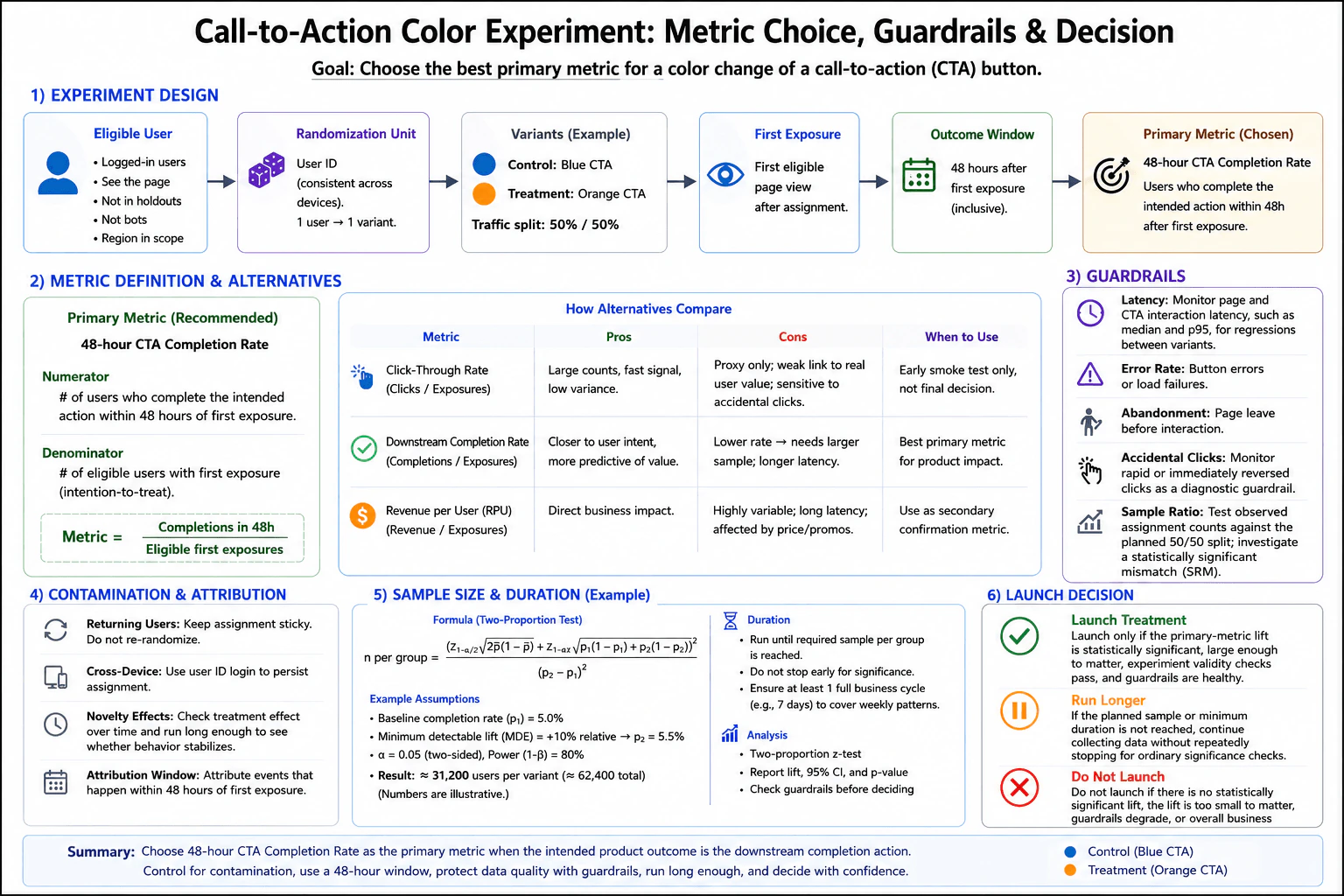
The color change should be judged by whether it helps users complete the intended action, not only whether it attracts more clicks. I would therefore use 48-hour CTA Completion Rate as the primary metric. An eligible user is a logged-in, in-scope, non-bot user who reaches the relevant page and is not excluded by a holdout. Randomize by user ID with sticky assignment. First exposure is the first eligible page view after assignment. Then count downstream completions during the next 48 hours and compare users according to their assigned variants.

Useful Questions to Ask the Interviewer
  1. What is the exact intended downstream action that the CTA should cause?
  2. Is the experiment population limited to logged-in users so assignment can remain stable across sessions and devices?
  3. Is a 48-hour attribution window appropriate for the normal time users need to complete the action?
  4. What baseline completion rate and minimum detectable effect should we use for power planning?
  5. Are there business constraints that should make revenue or another downstream measure part of the launch decision?
What primary metric would you choose for a call-to-action color experiment? diagram
How to Explain It in an Interview

Start with the user journey. The only treatment is CTA color. For each eligible user, assign one variant using user ID and keep that assignment sticky. The flow is: eligible user → randomization unit → assigned color variant → first eligible page view after assignment → 48-hour outcome window → primary metric.

Define the primary metric exactly. The numerator is the number of eligible users who complete the intended downstream action within 48 hours of first exposure. The denominator is the number of eligible users with first exposure. Analyze each exposed user according to the variant they were assigned. Do not condition the denominator on clicking, because clicking can itself be changed by the treatment.

I would prefer downstream completion over click-through rate when completion is the real product goal. Click-through rate has more events and often gives a faster, lower-variance signal, but it is only a proxy. A color can increase curiosity or accidental clicks without improving the real outcome. Revenue per user is closer to business value when monetization is the goal, but it can be much noisier and can be affected by price mix, promotions, refunds, and longer latency. I would normally use click-through rate as a diagnostic or early signal and revenue per user as a supporting business metric rather than automatically making either one primary.

Add guardrails so an apparent gain is not caused by a worse experience. Monitor page and CTA interaction latency, including median and p95, for regressions between variants. Track button errors or load failures. Track abandonment, such as leaving before interaction. Monitor rapid or immediately reversed clicks as an accidental-click diagnostic. These metrics do not replace the primary outcome, but they can block a launch if the treatment causes harm.

Protect experiment validity. Returning users must keep the same assignment; do not re-randomize them on later visits. When user identity is available across devices, use it to persist assignment. Compare observed assignment counts with the planned 50/50 split. A statistically significant deviation is a sample-ratio mismatch, or SRM, and should be investigated before trusting the treatment-effect estimate. Also inspect treatment effect over time because a new color can create a novelty response that later stabilizes or changes.

Use the fixed 48-hour attribution window consistently for both variants. An outcome belongs to the experiment when it occurs within 48 hours after that user's first exposure. The final analysis should wait until the included users' 48-hour outcome windows have matured so the groups are compared with complete outcome opportunity.

Plan sample size before running the experiment. Choose a baseline completion rate, significance level, desired power, and minimum detectable effect, or MDE. The MDE is the smallest improvement worth designing the experiment to detect. Using the diagram's illustrative assumptions, a 5.0% baseline, a 10% relative MDE corresponding to 5.5%, two-sided alpha of 0.05, and 80% power gives about 31,200 users per variant, or about 62,400 total under the shown two-proportion approximation. These are planning numbers, not observed experiment results.

Run until the planned sample size is reached and cover at least one full business cycle, such as a weekly cycle when weekly behavior matters. Do not repeatedly stop an ordinary fixed-horizon test as soon as a nominal p-value becomes significant. For the binary completion outcome, a two-proportion comparison is appropriate at the planned analysis point. Report the estimated lift, a 95% confidence interval, and the p-value, then interpret the effect size rather than relying on the p-value alone.

The launch rule combines statistical evidence and product judgment. Launch only when the primary-metric lift is statistically significant, large enough to matter, experiment-validity checks pass, and guardrails are healthy. If the planned sample size or minimum duration has not been reached, keep collecting data. Do not launch when there is no statistically significant lift, the estimated benefit is too small to matter, guardrails degrade, the experiment is invalid, or the overall business impact is negative.

Technical Approach
  1. Define the intended downstream action before choosing the metric.
  2. Define eligible users and exclusions before exposure.
  3. Randomize by user ID and keep assignment sticky across sessions and devices when possible.
  4. Assign each user to the control or treatment color variant according to the planned allocation.
  5. Define first exposure as the first eligible page view after assignment.
  6. Start a fixed 48-hour outcome window from first exposure.
  7. Use 48-hour CTA Completion Rate as the primary metric when downstream completion is the intended outcome: completions within 48 hours divided by eligible users with first exposure.
  8. Track click-through rate and revenue per user as supporting alternatives, not automatic replacements for the primary metric.
  9. Monitor latency, errors, abandonment, and accidental-click diagnostics as guardrails.
  10. Check returning-user consistency, cross-device assignment where possible, novelty over time, and sample-ratio mismatch against the planned allocation.
  11. Choose baseline rate, MDE, alpha, power, and required sample size before the test.
  12. Run to the planned sample and minimum duration, allowing the 48-hour outcome windows to mature.
  13. Estimate lift with uncertainty and check practical significance, validity checks, and guardrails before deciding whether to launch, run longer, or not launch.
Practical Insights

The metric itself is simple to compute, but trustworthy measurement has operational costs. A downstream completion metric usually needs more users than a click metric because completions are less frequent. A 48-hour window delays the final answer because late outcomes must mature. Sticky user assignment needs reliable identity, especially across devices. Guardrails and SRM checks add monitoring work but protect against bad launches. Revenue can be valuable but usually has higher variance and more business noise. A smaller MDE needs a larger sample and therefore more traffic or more time. Longer tests cost time, while shorter tests risk missing weekly patterns or overreacting to novelty.

Why Interviewers Ask This

This question tests whether the candidate can turn a simple UI experiment into a trustworthy causal measurement plan. The interviewer wants to see whether the candidate can define the population, randomization unit, exposure, attribution window, numerator, denominator, and primary outcome precisely. It also tests whether the candidate can distinguish an easy-to-move proxy such as clicks from a downstream user outcome, use guardrails, detect experiment-quality problems such as sample-ratio mismatch, plan power and duration, and make a launch decision using both statistical and practical significance.

Common interview mistakes

Common mistakes are choosing click-through rate just because it moves faster; failing to define the exact numerator, denominator, or 48-hour window; randomizing by page view instead of keeping a user in one variant; re-randomizing returning users; conditioning the denominator on users who clicked; ignoring cross-device contamination; using revenue as primary without considering its variance and latency; treating guardrails as optional; ignoring a statistically significant sample-ratio mismatch; looking at significance repeatedly and stopping early; choosing the MDE after seeing results; ending the experiment before outcome windows mature; and launching on statistical significance when the effect is too small to matter or guardrails have degraded.

Interview tip

Lead with one sentence naming the primary metric and why it matches the intended action. Then define eligibility, randomization, first exposure, numerator, denominator, and the 48-hour window precisely. Finish with metric alternatives, guardrails, SRM, MDE and duration, and a clear launch rule based on statistical significance, practical significance, validity, and user impact.
Interviewer may ask next
What would you do if the treatment increases CTA clicks but does not improve 48-hour downstream completion?

I would not call that a successful result if downstream completion is the intended outcome. The higher click rate shows that the new color changes interaction, but clicks are only a proxy. I would check accidental-click diagnostics, abandonment, latency, and errors to understand why the funnel is not improving. I would also verify assignment integrity and the 48-hour attribution logic. If the completion estimate remains flat after the planned sample and duration, I would not launch based only on the higher click-through rate.

What would you do if the primary metric looks positive but the experiment fails the sample-ratio check?

I would not trust the treatment-effect estimate until the sample-ratio mismatch is understood. I would compare observed assignment counts with the planned 50/50 allocation, then investigate causes such as inconsistent eligibility, missing logging, bot filtering, assignment bugs, or variant-specific failures. I would not repair the problem by simply reweighting the result without understanding the cause. If the SRM can bias which users appear in each arm and cannot be resolved reliably, I would treat the experiment as invalid and rerun it after fixing the assignment or data-quality problem.

2. How would you use propensity-score matching to estimate a recommender's effect on retention?Model Evaluation And ValidationMediumGoogle

Question Details

Users voluntarily opt into a recommender, and the outcome is seven-day retention. Available pre-treatment fields include user_id, prior watch behavior, prior sessions, country, and device. Define the treatment, outcome, ATT or ATE, and assumptions; build and validate the propensity model; enforce common support and a declared matching rule; evaluate standardized balance and remaining selection bias; estimate uncertainty; and compare matching with weighting, regression adjustment, doubly robust estimation, or a randomized design.

Short Interview Answer (30-60 seconds)

I would estimate each user's probability of opting into the recommender from pre-treatment covariates, restrict to common support, match opt-in users to similar non-opt-in users, verify standardized balance, and estimate the ATT on seven-day retention with valid uncertainty while acknowledging possible unmeasured confounding.

Detailed Explanation

The treatment is voluntary recommender opt-in: T=1 for users who opted in and T=0 otherwise. The outcome is a seven-day retention indicator. I would target the ATT, meaning the average effect for users who actually opted in. Because treatment is not randomized, I would use only pre-treatment information to estimate propensity scores, keep users in the region of common support, match comparable treated and control users, verify covariate balance, and then compare retention within the matched sample. The result is causal only under consistency/SUTVA, positivity, and no important unmeasured confounding.

Useful Questions to Ask the Interviewer
  1. Is the primary estimand the ATT for users who opted in, or do you want an ATE for the full eligible population?
  2. What exact product definition should be used for the seven-day retention indicator?
  3. Are prior watch behavior, prior sessions, country, and device all measured before the opt-in decision?
  4. Should unmatched treated users be excluded when common support is poor, and is 1:1 matching without replacement acceptable?
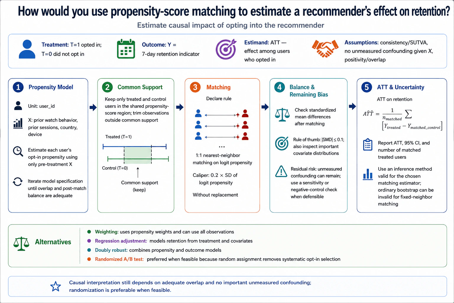
How would you use propensity-score matching to estimate a recommender's effect on retention? diagram
How to Explain It in an Interview
  1. Define treatment, outcome, and estimand. Treat recommender opt-in as T=1 and no opt-in as T=0. The outcome Y is seven-day retention. I would usually choose ATT = E[Y(1) - Y(0) | T=1], because the question naturally asks about the effect for users who actually opted in.
  1. State the causal assumptions. Consistency/SUTVA means each user's observed outcome corresponds to the treatment actually received and there is no relevant interference between users. No unmeasured confounding means that, after conditioning on the observed pre-treatment covariates X, treatment assignment is independent of the potential outcomes. Positivity means comparable treated and control users exist in the covariate region being analyzed.
  1. Build the propensity model. Use user_id only as the user-level identifier, not as a propensity-model covariate. Estimate each user's probability of opting in from prior watch behavior, prior sessions, country, and device. All of these variables must be measured before the opt-in decision. The goal is not simply to maximize treatment-prediction accuracy. The model should support adequate overlap and good balance of observed pre-treatment characteristics after matching.
  1. Enforce common support. Check whether treated and control users occupy a shared propensity-score region. Remove observations outside that overlap because they do not have credible counterparts. This changes the population represented by the estimate, so I would report how many treated users remain after trimming and matching.
  1. Declare the matching rule. Consistent with the diagram, I would use 1:1 nearest-neighbor matching without replacement on the logit of the propensity score, with a caliper of about 0.2 times the standard deviation of the logit propensity. If a treated user has no acceptable control within the caliper, I would leave that user unmatched rather than force a poor comparison.
  1. Validate balance after matching. Matching is not successful merely because the propensity model predicts opt-in well. I would calculate standardized mean differences for prior watch behavior, prior sessions, country, and device in the matched sample. An absolute SMD of about 0.1 or less is a useful rule of thumb, but I would also inspect important covariate distributions. If meaningful imbalance remains, I would revise the propensity specification or matching rule and repeat the balance check.
  1. Assess remaining selection bias. Good observed-covariate balance does not eliminate bias from variables that were not measured. I would state this limitation explicitly. Where defensible, I would add a sensitivity analysis or negative-control check to test how plausible remaining selection bias is.
  1. Estimate the ATT. For each matched treated user, compare observed retention with the retention of the matched control. Conceptually, ATT-hat = (1 / n_matched) * sum(Y_treated - Y_matched_control). Because retention is binary, this is an average difference in seven-day retention probability for the matched opt-in users.
  1. Report uncertainty correctly. Report the ATT, a 95% confidence interval, and the number of matched treated users. The inference procedure must be valid for the chosen matching estimator. I would not automatically use an ordinary nonparametric bootstrap for fixed-neighbor matching because that bootstrap can be invalid for this nonsmooth estimator.
  1. Compare alternatives. Propensity weighting can use all observations but may become unstable when propensity scores are very small or very large. Regression adjustment models retention from treatment and covariates and depends on outcome-model specification. A doubly robust method combines the propensity and outcome models and can remain consistent when one of those nuisance models is correctly specified, subject to the causal identification assumptions. If random assignment is feasible, an A/B test is preferable because randomization removes systematic opt-in selection.

The conclusion should remain conditional: propensity-score matching can provide an interpretable ATT when treated and control users have adequate overlap and good observed-covariate balance, but it cannot prove that important unmeasured confounding is absent.

Technical Approach
  1. Define T=1 as opting into the recommender and T=0 as not opting in; define Y as seven-day retention and choose ATT as the primary estimand.
  2. Use user_id as the user-level identifier and use only pre-treatment prior watch behavior, prior sessions, country, and device as propensity-model covariates.
  3. Estimate each user's propensity to opt in and iterate the model specification until overlap and post-match balance are adequate.
  4. Identify the shared propensity-score region and remove observations outside common support.
  5. Apply the declared rule: 1:1 nearest-neighbor matching without replacement on logit propensity with a caliper around 0.2 times its standard deviation.
  6. Measure post-match standardized mean differences and inspect important covariate distributions; revise the model or matching rule if balance is inadequate.
  7. Consider a sensitivity or negative-control analysis for remaining selection bias when defensible.
  8. Estimate the ATT from matched treated-control retention differences.
  9. Report ATT, a 95% confidence interval, the number of matched treated users, balance diagnostics, and limitations.
  10. Compare matching with weighting, regression adjustment, doubly robust estimation, and a randomized A/B test.
Practical Insights

The main cost is not just fitting the propensity model. Matching can discard users who have no comparable counterpart, so precision and generalizability may decrease when overlap is poor. Tighter calipers usually create more similar matches but can leave more treated users unmatched. Matching without replacement is simple to explain, but a particularly good control cannot be reused for several treated users. Balance checking and sensitivity analysis add analytical work but are essential because propensity scores alone do not prove that groups are comparable. Weighting keeps more data but can create unstable extreme weights. Regression and doubly robust methods add modeling assumptions. Randomization is usually the strongest design when it is feasible.

Why Interviewers Ask This

This question tests whether the candidate can turn voluntary product adoption into a defensible observational causal analysis. The interviewer wants to see correct treatment and outcome definitions, a clear estimand such as ATT, appropriate use of pre-treatment covariates, overlap and matching decisions, balance validation, uncertainty estimation, awareness of remaining selection bias, and judgment about when weighting, regression adjustment, doubly robust estimation, or randomization would be preferable.

Common interview mistakes

Common mistakes are treating user_id as a causal covariate instead of an identifier; using post-treatment behavior in the propensity model; choosing treatment-prediction AUC instead of post-match covariate balance as the main validation target; matching users with no common support; failing to declare the matching ratio, distance scale, caliper, or replacement rule; checking propensity scores but not standardized covariate balance; claiming that balanced observed covariates eliminate unmeasured confounding; reporting an ATT as though it were automatically an ATE for every user; forcing poor matches to keep sample size high; and using an ordinary bootstrap for fixed-neighbor matching without verifying that the inference method is valid.

Interview tip

Lead with the treatment, outcome, ATT, and assumptions. Then walk through propensity estimation, common support, matching, balance, remaining bias, and uncertainty. Emphasize that matching is judged by post-match covariate balance rather than treatment-prediction quality, and finish by stating the unmeasured-confounding limitation and why randomization is preferable when feasible.

Interviewer may ask next
What would you do if important covariates still have large standardized mean differences after matching?

I would not report the treatment effect from that matched sample as if the design were successful. I would revisit the propensity-model specification using the same pre-treatment covariates, consider justified nonlinear terms or interactions, and possibly adjust the caliper or matching strategy. Then I would repeat matching and recompute standardized mean differences and important covariate distributions. If acceptable balance still cannot be achieved, I would conclude that propensity-score matching is not giving a credible comparison for those users and consider weighting, regression adjustment, a doubly robust estimator, or a randomized design.

What if many opt-in users have propensity scores with no comparable non-opt-in users?

That is a positivity or common-support problem. I would not extrapolate from distant controls or force matches. I would restrict the analysis to the region where treated and control users overlap, report how many treated users were excluded, and make clear that the resulting ATT applies to the matched opt-in population rather than every opt-in user. If the excluded population is important, observational matching may not identify its effect credibly. Weighting may also become unstable in this situation, so collecting better comparison data or running a randomized A/B test would be preferable when feasible.

3. How would you compare the profits of two nearby stores rigorously?Model Evaluation And ValidationHardGoogle

Question Details

Two snack stores at the same school gate have 14 days of observations, and the decision concerns profitability in the next quarter. Define profit, passerby and open-hour denominators, transactions, average order value, margin, labor, rent, weather, school calendar, promotions, stockouts, and cannibalization. Design descriptive uncertainty and a controlled or quasi-experimental comparison that handles a change in hours, discounting, and a price change on day nine; assess power and sensitivity; and state a forward-looking decision rule rather than declaring a winner from raw totals.

Short Interview Answer (30-60 seconds)

I would define profit and normalize it by open hours and passerby exposure, then report uncertainty. I would prefer randomized store-by-time-block treatment. If that is impossible, I would use DiD only with a valid untreated store, credible pre-trends, and no material spillovers.

Detailed Explanation

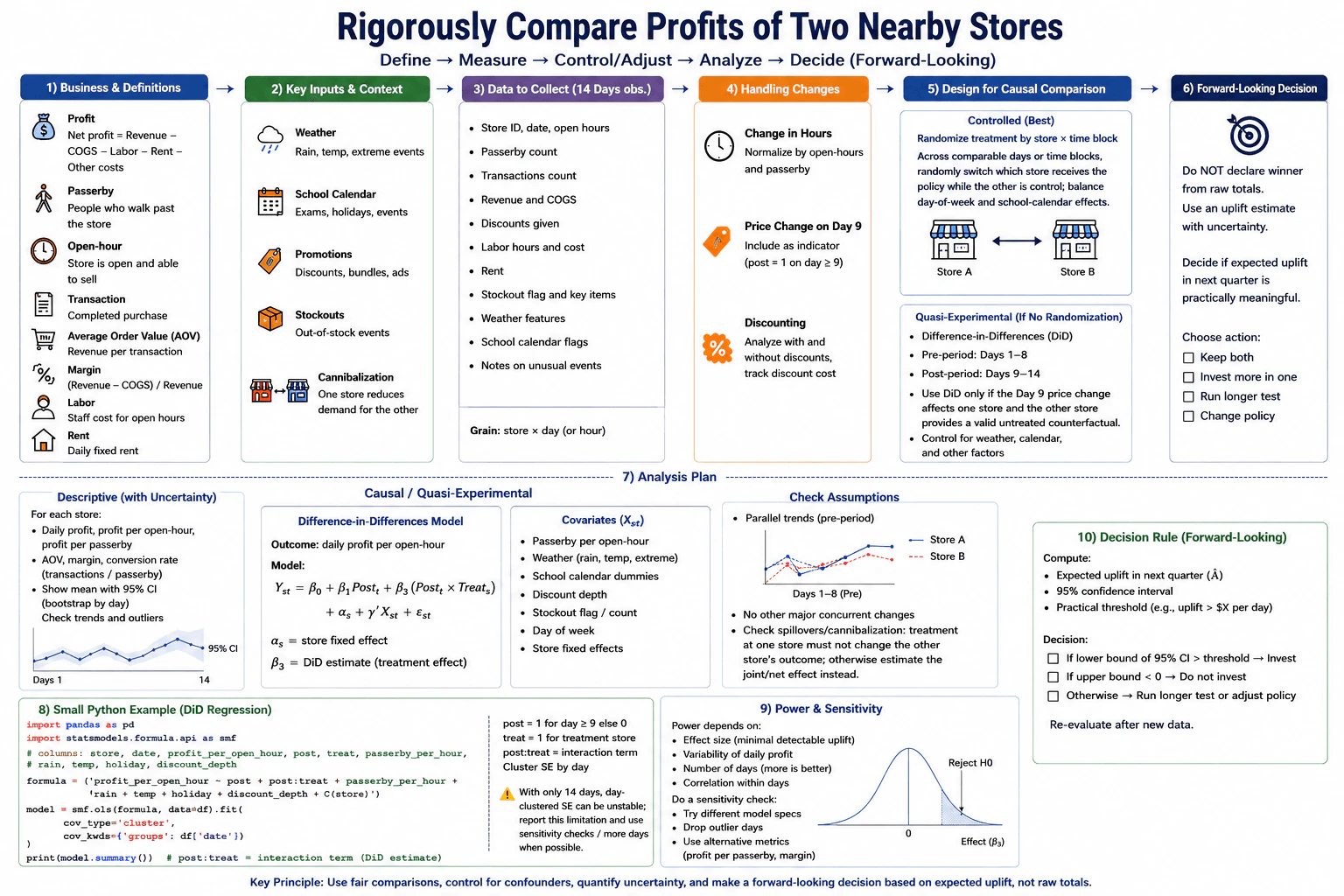
See the Code while reading this explanation.

I would compare normalized profit, not raw totals, because the stores may have different open hours and foot traffic. I would define profit and the exposure denominators first, then summarize both stores with uncertainty over the 14 observed days. For causal evidence, I would prefer randomized treatment by store and time block. If that is not possible, I would use Difference-in-Differences around the day-nine price change only when one store is untreated and the identifying assumptions are credible. The final decision should use expected next-quarter profit uplift, uncertainty, and a practical business threshold.

Useful Questions to Ask the Interviewer
  1. Did the day-nine price change happen at only one store, or at both stores?
  2. Can we randomize a pricing or promotion policy across comparable store-by-time blocks?
  3. Are passerby counts and actual open hours measured consistently for both stores?
  4. Were there other changes around day nine, such as promotions, staffing, stockouts, weather, or school events?
  5. What next-quarter profit uplift is large enough to justify changing the policy or investing more in one store?
How would you compare the profits of two nearby stores rigorously? diagram
How to Explain It in an Interview

Start by defining the outcome and denominators. Net profit is revenue minus cost of goods sold, labor, rent, and other operating costs. A passerby is a person who walks past the store. Open-hours are the hours when the store is actually open and able to sell. A transaction is a completed purchase. Average order value, or AOV, is revenue divided by transactions. Gross margin is (revenue minus cost of goods sold) divided by revenue.

Use a store-by-day grain, or store-by-hour if the data supports it. For both stores, collect open hours, passerby count, transactions, revenue, cost of goods sold, discounting, labor hours and cost, rent, stockouts, weather, school-calendar indicators, and unusual events. Record promotions and the day-nine price change explicitly. Because the stores are beside each other, also consider cannibalization: a change at one store may move demand away from the other.

First do descriptive analysis. Compare daily profit, profit per open-hour, profit per passerby, AOV, gross margin, and conversion rate, where conversion rate is transactions divided by passerby. Show trends and means with 95% confidence intervals, for example with a day-level bootstrap. This tells us how noisy the observed difference is. It does not by itself prove that one store or policy causes higher profit.

The preferred controlled design is to randomize the policy by store and time block across comparable days or time windows. Repeatedly switch which store receives the treatment while the other is the control. Balance important calendar factors such as day of week and school events. This is stronger than permanently calling one store treatment and the other control because store-specific differences are less likely to be confused with the policy effect.

If randomization is not possible, use Difference-in-Differences only if the day-nine price change affects one store and the other store is a credible untreated counterfactual. Use days 1-8 as the pre-period and days 9-14 as the post-period. A compact model is:

Y_st = β0 + β1 Post_t + β3(Post_t × Treat_s) + α_s + γ'X_st + ε_st

Here, Y_st is daily profit per open-hour, α_s is a store fixed effect, and β3 is the DiD estimate. X_st can include passerby per open-hour, weather, school-calendar indicators, stockouts, and day of week. Discount depth can also be included when it is a concurrent confounder; if discounting is itself the treatment or a consequence of treatment, do not control it away when estimating the total treatment effect.

The assumptions matter. The stores should have reasonably parallel pre-period trends. There should be no major one-sided concurrent change around day nine that is confused with the price change. Also check spillovers. If changing one store changes the other store's demand, the usual no-interference assumption is violated. Then the isolated store effect is hard to identify, and combined or net profit across both stores may be a better business outcome.

Power is a major limitation because there are only 14 observed days. Estimate the minimum detectable effect using the variability of daily profit, the number of days, and the correlation structure of repeated observations. With only 14 day clusters, cluster-robust inference can be unstable, so report that limitation and avoid presenting a narrow interval as definitive evidence.

Run sensitivity checks. Try reasonable alternative model specifications, remove or flag outlier days, vary defensible control sets, and repeat the analysis with alternative outcomes such as profit per passerby and margin. Check whether the sign and practical conclusion are stable. Also inspect missing or invalid observations, duplicate records, inconsistent open-hours, and broken passerby counts before fitting the model.

Finish with the decision rule. Estimate expected profit uplift for the next quarter and report a 95% confidence interval. Compare that uplift with a practical business threshold. If the lower bound of the interval is above the threshold, invest or adopt the better policy. If the upper bound is below zero, do not invest. Otherwise, run a longer test, collect more data, or adjust the policy. Do not declare a winner from the raw 14-day totals.

Key Insight / Why This Solution Works
  1. Define net profit, passerby, open-hours, transactions, AOV, gross margin, labor, rent, and conversion rate.
  2. Put both stores on the same store-by-day or store-by-hour grain.
  3. Validate missing, duplicate, and invalid observations, especially open-hours and passerby counts.
  4. Record weather, school calendar, promotions, stockouts, discounting, the day-nine price change, and possible cannibalization.
  5. Normalize outcomes by open-hours and passerby exposure where appropriate.
  6. Report descriptive trends, means, and 95% confidence intervals.
  7. Prefer randomized treatment by store and time block across comparable periods.
  8. If randomization is unavailable, use DiD only when one store is treated on day nine, the other is a valid untreated counterfactual, and pre-trends are credible.
  9. Model profit per open-hour with post, post-by-treatment interaction, store fixed effects, and defensible controls.
  10. Check concurrent changes, spillovers, outliers, alternative specifications, and alternative metrics.
  11. Assess minimum detectable effect and acknowledge that 14 days gives limited power.
  12. Estimate next-quarter uplift with uncertainty and apply the practical decision threshold rather than comparing raw totals.
Code
import pandas as pd
import statsmodels.formula.api as smf


def fit_store_did(df: pd.DataFrame):
    """Fit the quasi-experimental DiD model shown in the diagram."""
    required = {
        "date",
        "store",
        "profit_per_open_hour",
        "post",
        "treat",
        "passerby_per_hour",
        "rain",
        "temp",
        "holiday",
        "discount_depth",
    }
    missing = required.difference(df.columns)
    if missing:
        raise ValueError(f"Missing required columns: {sorted(missing)}")

    if df.empty:
        raise ValueError("Input data is empty.")

    work = df.copy()

    # One row per store and day for this implementation.
    if work.duplicated(["date", "store"]).any():
        raise ValueError("Duplicate store-date rows found.")

    # All model inputs must be observed so the cluster labels stay aligned.
    model_columns = sorted(required)
    if work[model_columns].isna().any().any():
        raise ValueError("Model columns must not contain missing values.")

    if not set(work["post"].unique()).issubset({0, 1}):
        raise ValueError("post must contain only 0 or 1.")
    if not set(work["treat"].unique()).issubset({0, 1}):
        raise ValueError("treat must contain only 0 or 1.")
    if work["post"].nunique() < 2:
        raise ValueError("Both pre-period and post-period observations are required.")
    if work["treat"].nunique() < 2:
        raise ValueError("Both treated and untreated stores are required.")
    if work["date"].nunique() < 2:
        raise ValueError("At least two date clusters are required.")

    formula = (
        "profit_per_open_hour ~ post + post:treat + passerby_per_hour + "
        "rain + temp + holiday + discount_depth + C(store)"
    )

    model = smf.ols(formula, data=work).fit(
        cov_type="cluster",
        cov_kwds={"groups": work["date"]},
    )
    return model
Why Interviewers Ask This

This tests whether the candidate can turn a short, messy observational comparison into a defensible business decision. The interviewer is looking for clear metric definitions, fair denominators, causal-design judgment, treatment of confounders and spillovers, uncertainty and power analysis, sensitivity checks, and a forward-looking rule that does not overclaim from only 14 days.

Common interview mistakes

Common mistakes are comparing raw 14-day profit totals, ignoring different open hours or passerby traffic, treating AOV as profit, forgetting labor or rent, ignoring discount cost and stockouts, calling a simple day-nine before/after comparison causal without a valid untreated store, using DiD without checking pre-trends, controlling for a variable that is actually part of the treatment, ignoring cannibalization, overtrusting clustered inference with only 14 days, and choosing a winner from a point estimate without uncertainty or a practical next-quarter threshold.

Interview tip

Lead with the decision, then move in this order: define profit, normalize exposure, quantify uncertainty, choose the strongest feasible causal design, state its assumptions, discuss power and sensitivity, and finish with the forward-looking decision rule.

Interviewer may ask next
What would you do if the two stores do not have parallel trends during days 1-8?

I would not treat the basic DiD estimate as credible. I would look for a better comparison period or, preferably, run a randomized store-by-time-block test. I could model pre-period trends as a sensitivity check, but eight pre-days provide weak evidence. If no defensible counterfactual exists, I would describe the observed difference without making a causal claim and collect more data.

What if the estimated next-quarter uplift is positive, but its 95% confidence interval crosses both zero and the practical threshold?

I would not make a strong invest-or-do-not-invest claim. The point estimate may be positive, but the evidence is too uncertain relative to the business threshold. I would run a longer test or collect more days using the same outcome and decision rule. If waiting is costly, I would make that decision cost explicit instead of pretending the 14-day evidence is decisive.

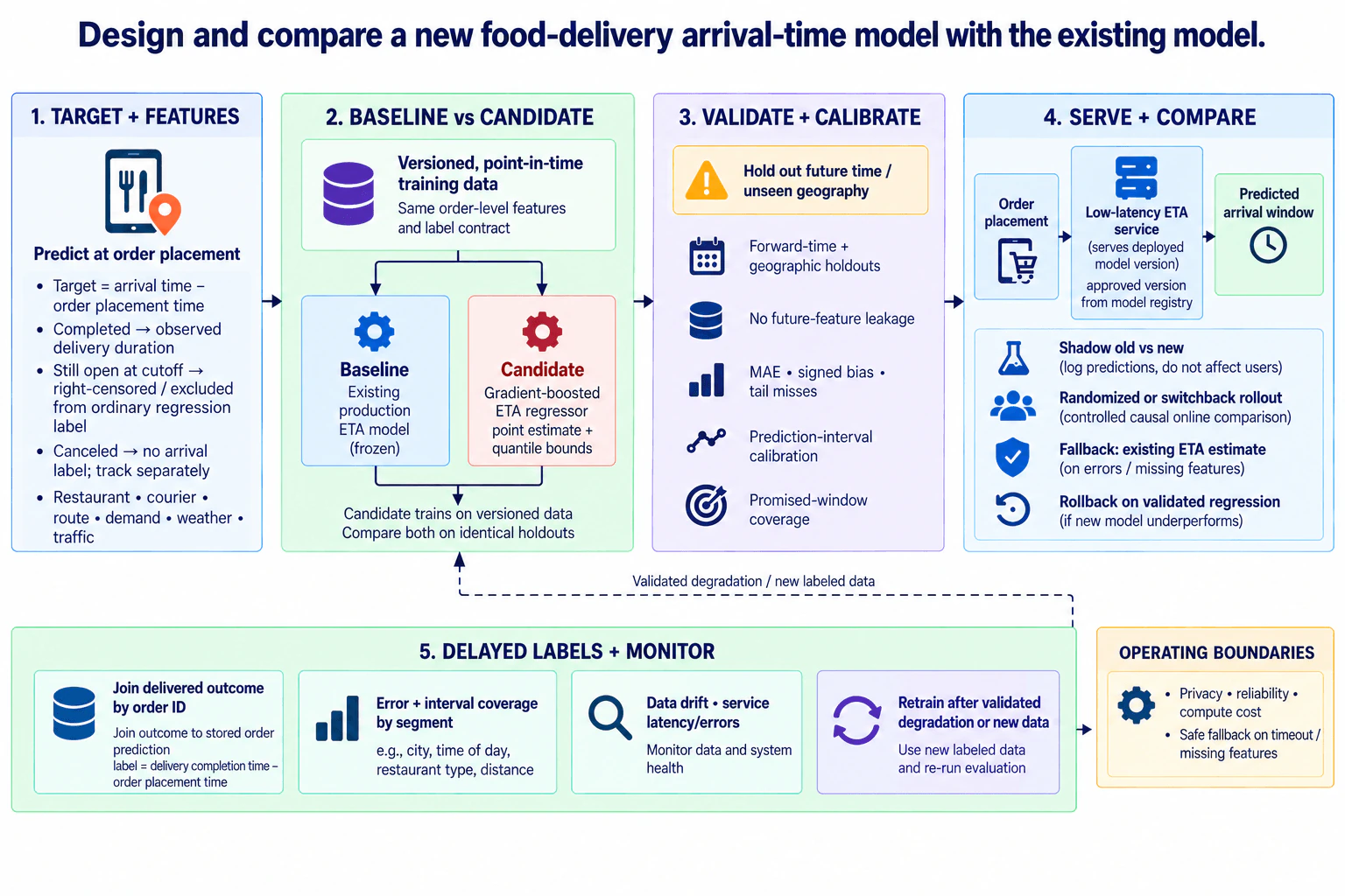
4. Design and compare a new food-delivery arrival-time model with the existing model.NEWMachine Learning System DesignEasyGoogle

Question Details

Design the model and evaluation path for predicting delivery time at order placement. Define the order-level target, prediction timestamp, censoring and cancellation rules, restaurant, courier, route, demand, weather, and traffic features, baseline and candidate models, geographic and temporal validation, calibration of prediction intervals, and metrics for absolute error, bias, tail misses, and promised-window coverage. Connect versioned training data and a registry to low-latency serving, shadow comparison, randomized or switchback rollout, fallback estimates, delayed-label feedback, drift and segment monitoring, retraining, rollback, privacy, reliability, and compute cost.

Short Interview Answer (30-60 seconds)

I would predict delivery duration at order placement, keep the current ETA model frozen as the baseline, and train a versioned candidate on point-in-time features. I would compare both on identical temporal and geographic holdouts, then use shadow and controlled rollout before promotion, with fallback, rollback, and delayed-label monitoring.

Detailed Explanation

The prediction is made once per food-delivery order at order placement. The target is delivery completion time minus order placement time, using only information available at that moment. I would keep the current production ETA model frozen as the baseline, train a versioned candidate on point-in-time features, and compare both on identical future-time and geographic holdouts. I would validate average error, bias, tail misses, and arrival-window coverage, then use shadow and controlled online rollout before promotion. Serving needs fallback, rollback, delayed-label joins, monitoring, and retraining gates.

Useful Questions to Ask the Interviewer
  1. Is the customer-facing output a point ETA, an arrival window, or both?
  2. For orders still open at the labeling cutoff, should we use a censoring-aware model or exclude them until completion?
  3. Which geographic regions and future periods should be reserved for generalization testing?
  4. Is ordinary randomized rollout acceptable, or does marketplace interference make a switchback design preferable?
  5. What serving failures must trigger fallback to the existing ETA estimate?
Design and compare a new food-delivery arrival-time model with the existing model. diagram
How to Explain It in an Interview

Start with the prediction contract. The prediction unit is one order, and the prediction timestamp is order placement. For a completed order, the regression label is delivery completion time - order placement time. Orders still open at the labeling cutoff do not yet have a completed regression label; they are right-censored if the modeling method supports censoring, or excluded from ordinary regression training until the outcome arrives. Canceled orders have no arrival label and should be tracked separately.

Next, build versioned point-in-time training data. Restaurant, courier, route, demand, weather, and traffic features must reflect what was known at order placement. This prevents future-feature leakage and training-serving skew. Store the data snapshot, feature definitions, training configuration, model artifact, and evaluation result so a model version can be reproduced and traced.

Keep the existing production ETA model frozen as the baseline. Train the candidate, shown in the diagram as a gradient-boosted ETA regressor, on the versioned training data. If the product exposes an arrival window, train quantile bounds or another interval-producing variant and calibrate the interval on held-out data. The baseline and candidate must be compared on the same evaluation examples and the same label contract.

Use forward-time validation so training examples precede validation examples. Add geographic holdouts to test generalization to unseen areas. Evaluate MAE for typical absolute error, signed bias for systematic early or late predictions, tail misses for severe errors, and promised-window coverage for uncertainty quality. Promotion should require passing this validation gate; a lower training loss alone is not enough.

After offline approval, register the candidate version and deploy that approved version to a low-latency ETA service. First run shadow comparison: log the old and new predictions for the same requests without changing the user-visible estimate. Then use a controlled online experiment. Use randomized rollout when the treatment units are sufficiently independent; use a switchback design when marketplace interference or shared operational conditions make simultaneous user-level randomization inappropriate.

Serving must fail safely. If the new service times out, required features are missing, or the candidate cannot serve a prediction, return the existing ETA estimate. Keep the previous model version available so a validated regression can trigger rollback. Monitor service latency and errors separately from model quality.

The true outcome arrives later. Join the delivered outcome back to the stored prediction by order ID, prediction timestamp, and model version. Recompute delivery completion time - order placement time as the delayed label. Monitor error and prediction-window coverage by segments such as city, time of day, restaurant type, and distance. Monitor data drift and system health as separate signals; drift alone does not prove that prediction quality has worsened.

Retrain when enough new labeled data is available or when monitoring identifies a validated degradation. The retrained candidate must pass the same point-in-time, temporal, and geographic validation gate before deployment. Throughout the system, keep privacy, reliability, and compute cost as operating boundaries: retain only needed data, protect sensitive fields, maintain a safe fallback path, and avoid model complexity whose accuracy benefit does not justify its training and serving cost.

Technical Approach
  1. Define one prediction per order at order placement and the target as delivery completion time minus order placement time.
  2. Use completed orders as observed labels. Treat still-open orders as right-censored when supported, or exclude them from ordinary regression training until completion. Track canceled orders separately.
  3. Build versioned point-in-time restaurant, courier, route, demand, weather, and traffic features using only information available at prediction time.
  4. Freeze the existing production ETA model as the baseline and train the gradient-boosted candidate on the versioned data, including quantile bounds when an arrival window is needed.
  5. Compare baseline and candidate on identical forward-time and geographic holdouts.
  6. Evaluate MAE, signed bias, tail misses, prediction-interval calibration, and promised-window coverage.
  7. Register only a candidate that passes the offline validation gate, then deploy the approved version to the low-latency ETA service.
  8. Run shadow comparison before changing user-visible estimates.
  9. Use randomized rollout when units are sufficiently independent, or switchback rollout when interference makes ordinary randomization unreliable.
  10. Fall back to the existing ETA estimate on timeout, missing features, or serving failure, and roll back on validated regression.
  11. Join delayed delivery outcomes to stored predictions by order ID, prediction timestamp, and model version.
  12. Monitor segment error, interval coverage, data drift, latency, and errors. Retrain on new labeled data or validated degradation, then repeat the same validation gate.
Time & Space Complexity

The hardest cost is often trustworthy evaluation, not model fitting. Temporal and geographic holdouts reduce the amount of data available for training, but they give a more realistic generalization test. Quantile bounds and calibration add training and validation work, but they make an arrival window more meaningful. A larger gradient-boosted model can improve accuracy while increasing CPU use and serving latency. Shadowing can roughly duplicate inference work for compared requests. Controlled experiments take time and may need switchback designs when marketplace interference exists. Keeping the baseline available for fallback and rollback adds operational complexity, but it reduces reliability risk. Prediction logging, delayed-label joins, segment monitoring, and retraining also add storage, compute, and maintenance cost.

Where it is used

This approach is useful for real-time ETA systems where a prediction is made before the outcome is known, conditions vary across geography and time, uncertainty matters to the user-facing promise, and a new model must be compared safely with an existing production model before full rollout.

Why Interviewers Ask This

This question tests whether a candidate can design a complete production ML system, not just fit a regression model. The key judgments are label and feature timing, leakage prevention, fair baseline comparison, temporal and geographic generalization, uncertainty calibration, safe online experimentation, low-latency serving, delayed-label feedback, segment monitoring, fallback and rollback, plus privacy, reliability, and compute-cost tradeoffs.

Common interview mistakes

Common mistakes are using features that were not available at order placement, leaking future information into training, giving still-open or canceled orders fake completed labels, comparing models on different holdouts, retraining the production baseline instead of freezing it for comparison, relying only on random splits, reporting only MAE while ignoring bias and tail misses, producing arrival windows without checking coverage, confusing the model registry with the online serving service, deploying directly from offline metrics without shadow or controlled rollout, assuming drift alone proves model degradation, failing to join delayed outcomes to the original order prediction and model version, and omitting fallback or rollback behavior.

Interview tip

Present the system as five decisions: define the order-level target and feature timing, compare frozen baseline versus candidate, validate and calibrate on future and geographic holdouts, serve through shadow plus controlled rollout with fallback, then close the loop with delayed-label monitoring and retraining.

Interviewer may ask next
How would you handle orders that are still in progress when the training snapshot is created?

Their completed delivery duration is not known yet, so I would not assign a fabricated regression label. If the chosen modeling method supports censoring, I would retain them as right-censored observations. Otherwise, I would exclude them from the ordinary regression training set until they complete. I would keep the order ID, prediction timestamp, and model version so the completed outcome can later be joined back correctly. Canceled orders remain separate because they never produce an arrival label.

What if the candidate improves MAE but worsens tail misses or promised-window coverage?

I would not promote it automatically. Lower average error does not justify more severe misses or a less reliable user-facing arrival window. I would inspect the affected segments, recalibrate or retrain the candidate if appropriate, and rerun the same temporal and geographic validation. If the tradeoff remains unacceptable, I would keep the existing production model and continue iterating.

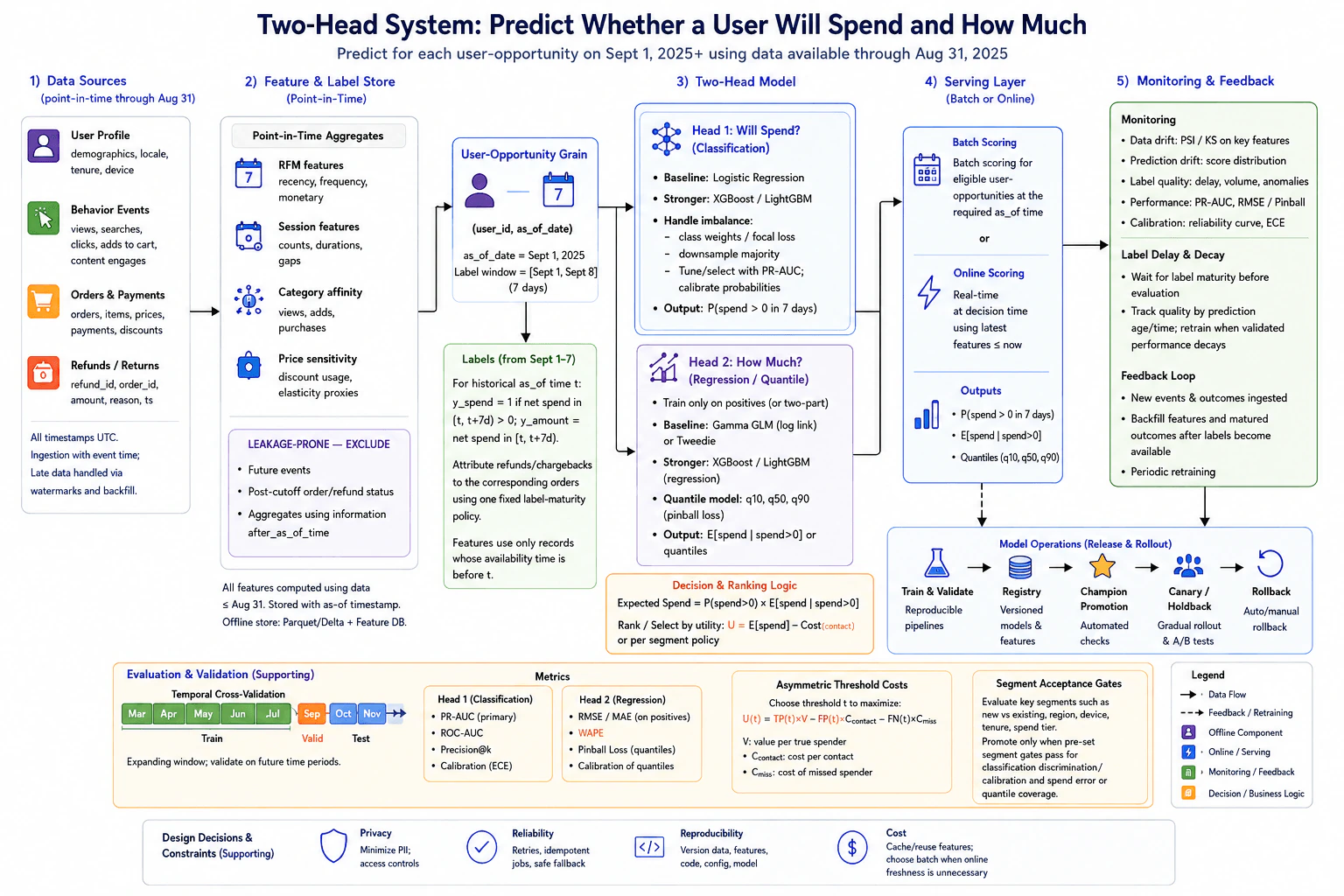
5. Design a two-head system that predicts whether a user will spend and how much.Machine Learning System DesignMediumGoogle

Question Details

For predictions beginning September 1, 2025, use events and orders available through August 31 to predict both the probability of any spend in the next seven days and the expected or quantile spend. Define user-opportunity grain, label windows, refund handling, point-in-time aggregates, leakage-prone fields, classification and regression baselines, imbalance handling, temporal cross-validation, calibration, asymmetric threshold costs, and segment acceptance gates. Design versioned data and features, reproducible training, registry promotion, batch or online serving, holdback rollout, monitoring for drift, label delay and decay, feedback, retraining, rollback, privacy, reliability, and cost.

Short Interview Answer (30-60 seconds)

I would score each user-opportunity at an as-of time using only information available before that boundary. One head predicts seven-day spend probability and the other predicts conditional amount or quantiles. I would use temporal validation, calibration, cost-aware segment gates, versioned promotion, and monitored batch or online serving.

Detailed Explanation

The prediction unit is one user-opportunity at an as-of time. For the September 1, 2025 opportunity, features use records available before that boundary, which means data available through August 31, while the seven-day label window is [September 1, September 8). Head 1 estimates the probability that net spend is positive. Head 2 estimates spend conditional on spending, or conditional quantiles such as q10, q50, and q90. The system must keep features point-in-time correct, handle refunds consistently, validate on later time periods, calibrate probabilities, apply business-aware decision gates, and preserve those contracts in serving and monitoring.

Useful Questions to Ask the Interviewer
  1. Is one prediction required per user per day, or only when a specific user opportunity occurs?
  2. Should the second head optimize conditional expected spend, conditional spend quantiles, or both?
  3. Are decisions made in scheduled batches, in real time, or through both paths?
  4. Which user segments require separate acceptance checks before model promotion?
  5. How should refunds and chargebacks be attributed, and when is a label considered mature enough for evaluation?
  6. What business values define the cost of an unnecessary action and the cost of missing a likely spender?
Design a two-head system that predicts whether a user will spend and how much. diagram
How to Explain It in an Interview

Start with the data contract. Each record is keyed by user and as-of time. For the September 1 prediction, the system can use user profile data, behavior events, orders and payments, and refunds or returns whose information is available before the prediction boundary. From these sources, compute point-in-time aggregates such as recency, frequency, monetary behavior, session features, category affinity, and price-sensitivity signals. Explicitly exclude future events, post-cutoff order or refund status, and aggregates that use information after the as-of time. The same feature definitions and availability rules must be used during training and serving to avoid leakage and training-serving skew.

Define labels at the same grain. For a historical as-of time t, set y_spend = 1 when net spend in [t, t+7d) is greater than zero, otherwise 0. Set y_amount to net spend in that same interval. Attribute refunds and chargebacks to the corresponding orders using one fixed label-maturity policy. Because outcomes can be revised after the original transaction, evaluation should wait until the required labels are mature enough for a fair comparison.

For Head 1, use logistic regression as an interpretable baseline and compare it with a stronger tree model such as XGBoost or LightGBM. If positive spend is rare, handle imbalance with class weighting, focal loss, or majority downsampling as appropriate. Use PR-AUC to compare or tune models rather than treating it as a differentiable loss. After choosing the model, calibrate its probabilities and verify calibration on future validation data.

For Head 2, train on positive-spend cases in the two-part design. A Gamma GLM with a log link or a Tweedie model is a reasonable baseline when its assumptions fit the data. A boosted-tree regressor such as XGBoost or LightGBM can model stronger nonlinear effects. If uncertainty matters, train conditional quantile models such as q10, q50, and q90 using pinball loss. The head returns E[spend | spend > 0] or conditional spend quantiles.

When an unconditional expected-spend score is useful, combine the heads as E[spend] = P(spend > 0) × E[spend | spend > 0]. That score can support ranking or selection. If taking an action has asymmetric costs, choose the operating threshold by expected utility rather than automatically using 0.5. A compact form is U(t) = TP(t) × V - FP(t) × C_contact - FN(t) × C_miss, where V is the value of correctly identifying a spender, C_contact is the cost of an unnecessary contact, and C_miss is the cost of missing a spender. Those values must come from the business context rather than being invented.

Validation must respect time. Use expanding-window or rolling temporal cross-validation so training uses older data and validation uses later data. Keep the final test period after the tuning periods. For Head 1, evaluate PR-AUC, ROC-AUC, precision at the relevant operating point, and calibration such as expected calibration error. For Head 2, evaluate RMSE or MAE on positive-spend cases, WAPE when appropriate for the reporting need, pinball loss for quantile models, and quantile calibration or coverage. Never promote a model based only on a training metric.

Promotion should also use pre-set segment acceptance gates. Evaluate important segments such as new versus existing users, region, device, tenure, and spend tier. Promote only when the required classification discrimination and calibration checks plus spend-error or quantile-coverage checks pass for the required segments. This prevents an aggregate improvement from hiding a harmful regression in a meaningful population.

Make training reproducible. Version the data, feature definitions, code, configuration, model artifact, and evaluation results. Store the approved model and feature versions in a registry with their lineage. Promotion moves a validated challenger to the serving path only after the configured checks pass. Use a canary or holdback rollout so part of the eligible population can remain on the prior champion during evaluation. Keep the previous approved version available for rollback.

Serving can be batch or online. Batch scoring computes predictions for eligible user-opportunities at the required as-of time. It is usually the lower-cost choice when immediate freshness is unnecessary. Online scoring computes a prediction at decision time using the latest features that are valid and available then. Both paths must use compatible feature definitions, schemas, and prediction contracts. If the online path experiences stale or missing features, timeouts, overload, or a missing model, invoke the predefined safe fallback policy instead of silently returning an invalid prediction, and retain rollback to the previous approved model.

Monitoring should separate different kinds of problems. Track service health such as latency, errors, retries, timeouts, and overload separately from data quality. Track key-feature drift with measures such as PSI or KS when appropriate, prediction-score drift, missing or delayed data, and label-volume anomalies. Track classification quality, calibration, spend error, pinball loss or quantile coverage, and the relevant business outcome after labels mature. Drift is a warning signal, not proof that model quality has declined.

The feedback loop joins realized spend, refunds, and other matured outcomes back to the original prediction using the correct user-opportunity and as-of time. Backfill matured labels and the corresponding historical features after delayed information becomes available. Retrain on the agreed schedule or when validated performance decay justifies it, then repeat temporal validation and segment gates before promotion. Keep rollback available throughout the lifecycle.

Finally, keep privacy, reliability, reproducibility, and cost explicit. Minimize personally identifiable information and enforce access controls. Use retries and idempotent jobs where appropriate, with a defined safe fallback for failures. Version the complete lineage so results can be reproduced. Reuse or cache features when that reduces repeated work without breaking point-in-time correctness. Prefer batch inference when online freshness is unnecessary. The main point is that the two model heads are only part of the design; trustworthy predictions depend on correct time boundaries, reproducible validation, controlled promotion, and a production feedback loop.

Technical Approach
  1. Define one record per user-opportunity and as-of time.
  2. For the September 1, 2025 opportunity, use only information available before that boundary and define the outcome window as [September 1, September 8).
  3. Build point-in-time profile, behavior, RFM, session, category-affinity, and price-sensitivity features; exclude future and post-cutoff information.
  4. Create refund-aware y_spend and y_amount labels with one fixed label-maturity policy.
  5. Train Head 1 with logistic regression as a baseline and a boosted-tree classifier as a stronger candidate; handle imbalance with weighting, focal loss, or downsampling.
  6. Train Head 2 on positive-spend cases using a conditional mean model or conditional quantile model; compare a simple regression baseline with a boosted-tree alternative.
  7. Calibrate Head 1 probabilities and combine the two heads as P(spend > 0) × E[spend | spend > 0] when unconditional expected spend is needed.
  8. Use rolling or expanding temporal cross-validation. Evaluate classification, calibration, amount error, and quantile quality on future periods.
  9. Choose decision thresholds with asymmetric business costs and require pre-set acceptance gates for important segments.
  10. Version data, features, code, configuration, models, and evaluation artifacts. Promote only validated candidates through the model registry.
  11. Serve through batch scoring, online scoring, or both while preserving the same feature and prediction contracts.
  12. Roll out with a holdback or canary. Monitor service health, data quality, drift, calibration, delayed-label quality, and business outcomes. Retrain after validated decay or on the agreed schedule, and use safe fallback or rollback when production checks fail.
Practical Complexity & Trade-offs

The main cost comes from computing point-in-time features, training two model heads, storing versioned artifacts, validating across multiple time windows, and serving predictions. Batch scoring is usually simpler and cheaper because many users can be processed together, but it may use less-fresh information. Online scoring gives fresher decisions but needs low-latency feature access, timeout and overload handling, and a safe fallback when valid features or models are unavailable. Temporal cross-validation costs more than one random split because training is repeated across time windows, but it better represents future behavior. Quantile models add more training and monitoring work because several outputs must be checked for calibration or coverage. Shared or cached feature computation can reduce cost as long as point-in-time correctness is maintained.

Where it is used

This design is useful when a product needs both the probability of near-term spending and an estimate of how much a spender may spend. It can support prioritizing user opportunities for a limited action, ranking opportunities by expected spend, short-horizon value forecasting, or making a cost-aware decision where contacting the wrong user and missing a likely spender have different consequences. The two-part structure is especially useful when many users have zero spend because the zero-versus-positive event is modeled separately from the positive amount.

Why Interviewers Ask This

This tests whether I can connect statistical modeling with production machine-learning system design. The important judgment is not just choosing two models. I must define the prediction grain and time boundaries correctly, prevent leakage, create refund-aware labels, handle class imbalance, validate on future periods, calibrate probabilities, choose thresholds using asymmetric business costs, and require acceptable quality across important user segments. I also need to show reproducible and versioned training, registry-based promotion, compatible batch and online serving, delayed-label monitoring, feedback, retraining, privacy, reliability, cost control, safe degradation, and rollback.

Common interview mistakes

Common mistakes are using a random train-test split instead of temporal validation; allowing future events, post-cutoff order status, or refunds to leak into features; using different feature availability rules in training and serving; defining inconsistent label-window boundaries; training the conditional amount head without explaining the positive-spend population; treating PR-AUC as a differentiable training loss; reporting only aggregate metrics and ignoring calibration or segment regressions; choosing a 0.5 threshold without asymmetric-cost analysis; treating drift alone as proof that model quality declined; evaluating before delayed outcomes mature; joining feedback to the wrong user-opportunity or time; promoting directly from a training metric without versioned evaluation and registry gates; and having no explicit handling for stale features, timeouts, overload, missing models, safe fallback, or rollback.

Interview tip

Start with the grain and time boundary before naming any model. State the feature cutoff and seven-day label window, then explain the two heads, temporal validation, calibration, asymmetric-cost and segment gates, versioned promotion, serving, delayed-label feedback, safe fallback, and rollback. That ordering makes leakage prevention and production judgment easy to see.

Interviewer may ask next
How would you handle refunds or chargebacks that arrive after the seven-day spend window?

I would define one label-maturity policy before training. The prediction target still uses the seven-day outcome window [t, t+7d), but the historical net-spend label is not treated as final until the refund or chargeback information required by that policy has matured. Historical labels are built consistently with that rule, and production quality is evaluated only after the matching label is mature. I would also monitor label delay and revision behavior. Information that becomes known later must never leak into features for the earlier as-of time.

What would you change if the business suddenly required a real-time decision instead of batch scoring?

I would keep the same user-opportunity, label, and model contracts but use the online serving path. The online feature path must return only values that are valid and available at the decision time and must use feature definitions compatible with training. I would make latency, timeouts, overload, stale features, and missing-model behavior explicit operational checks. If a valid prediction cannot be produced, the system should invoke its predefined safe fallback policy rather than fabricate a score. Temporal validation, calibration, segment acceptance gates, holdback rollout, monitoring, feedback, and rollback still apply.

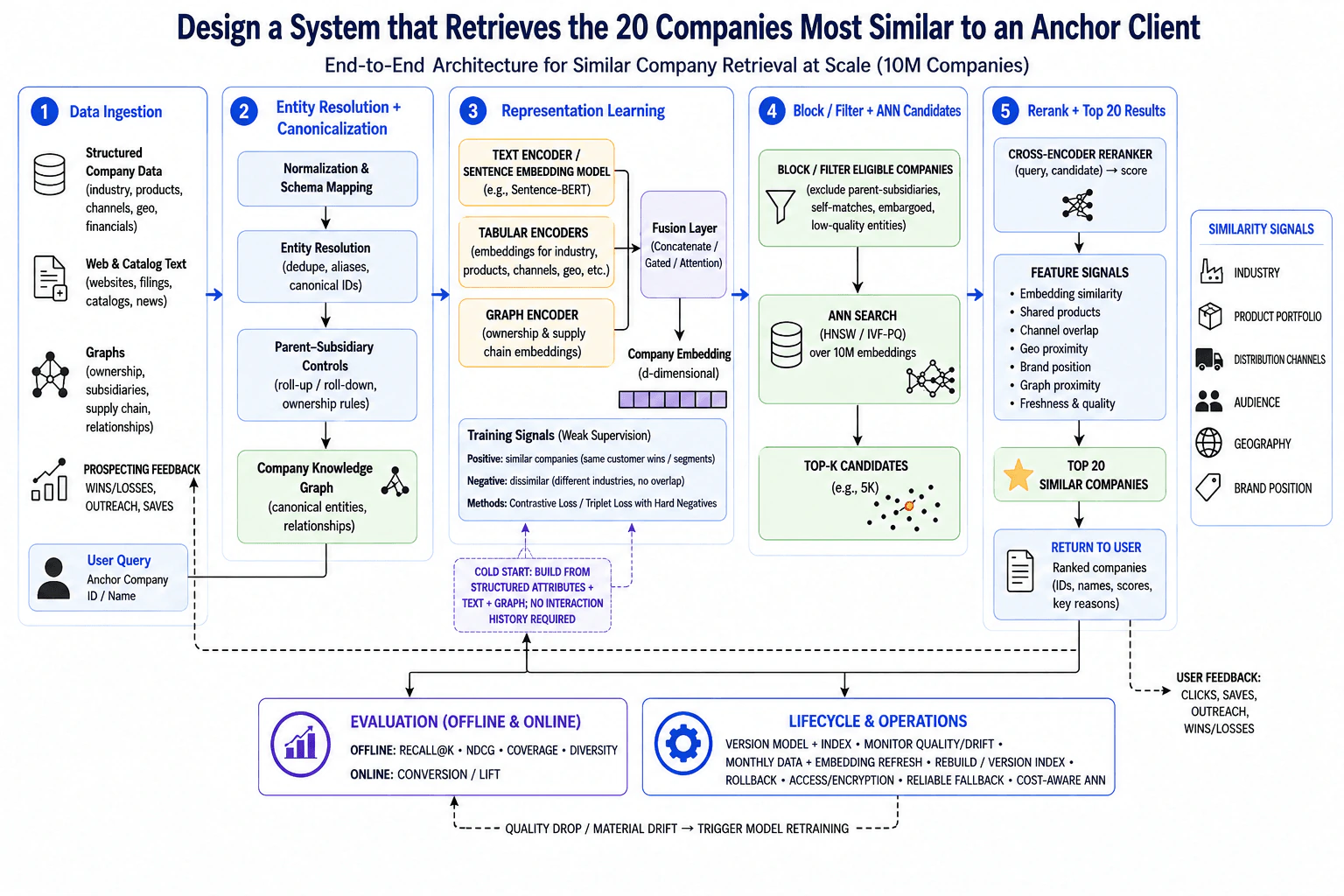
6. Design a system that retrieves the 20 companies most similar to an anchor client.Machine Learning System DesignHardGoogle

Question Details

Define similarity for global sales prospecting across industry, product portfolio, distribution channels, audience, geography, and brand position. Design ingestion of structured company attributes, web and catalog text, and ownership or supply-chain graphs; entity resolution and parent-subsidiary controls; weak supervision, contrastive or triplet representation learning; blocking, approximate-nearest-neighbor candidate generation and reranking for 10 million companies; monthly updates and cold start; versioned indexes and models; Recall@K, NDCG, coverage, diversity and online conversion evaluation; serving, monitoring, feedback, drift-triggered retraining, privacy, security, reliability, rollback, and cost.

Short Interview Answer (30-60 seconds)

I would canonicalize each company, learn one representation from structured, text, and graph signals, block ineligible entities, and run ANN search over 10 million embeddings. I would rerank the Top-K candidates to return 20, then use monthly refreshes, offline and online evaluation, feedback, drift-triggered retraining, versioning, monitoring, and rollback.

Detailed Explanation

The goal is to return 20 useful company analogs for one anchor client in global sales prospecting. Similarity is multi-faceted, so I would represent industry, product portfolio, distribution channels, audience, geography, and brand position instead of relying on one field. The system must combine structured company data, web and catalog text, and ownership or supply-chain graphs, remove duplicate or inappropriate parent-subsidiary matches, and search efficiently across 10 million companies. It also needs monthly freshness, cold-start support, measurable retrieval quality, business feedback, safe versioning, monitoring, security, reliability, cost control, and rollback.

Useful Questions to Ask the Interviewer
  1. Should parent and subsidiary companies ever be returned together, or should the system normally collapse them to one corporate family?
  2. Are all six similarity dimensions equally important for every prospecting use case, or may their importance vary by context?
  3. Is the user always querying with a known canonical company ID, or must the service also resolve a company name or profile at request time?
  4. Is the required monthly refresh sufficient for all company attributes, or are some sources expected to update more frequently?
  5. Which online outcome should be the primary business objective: conversion, qualified outreach, saves, wins, or another prospecting event?
Design a system that retrieves the 20 companies most similar to an anchor client. diagram
How to Explain It in an Interview
1. Define the ranking problem

The unit being ranked is a canonical company. The request contains one anchor company, and the output is an ordered list of 20 other eligible companies.

Similarity comes from six groups of evidence: industry, product portfolio, distribution channels, audience, geography, and brand position. I would not force one permanent hand-written weighted formula. These signals feed the learned representation and reranker so their importance can be learned from weak supervision and prospecting feedback.

2. Build a canonical company view

The offline pipeline ingests structured company attributes, web and catalog text, and ownership or supply-chain graphs. Prospecting feedback such as wins, losses, outreach, clicks, and saves provides weak supervision and later online evaluation signals.

Before modeling, I normalize fields, deduplicate aliases, and assign a canonical company ID. I also maintain parent-subsidiary relationships. These controls matter because the anchor itself, a duplicate record, or an inappropriate company from the same corporate family may look highly similar while being useless as a prospect.

3. Learn a multi-modal representation

I create a sentence-level text representation from company descriptions and catalog content, tabular representations from attributes such as industry, products, channels, audience, and geography, and graph representations from ownership and supply-chain relationships. A fusion layer combines these signals into one company embedding.

For weak supervision, positive pairs can come from companies associated with similar customer wins or segments. Negatives can come from clearly dissimilar companies, and hard negatives can be mined from companies that look superficially similar but should not rank highly. I train the representation with a contrastive or triplet objective so useful analogs move closer in embedding space and dissimilar companies move farther apart.

4. Support cold start

A new company may have no interaction history. I still build its representation from structured attributes, text, and graph information, exactly as in the diagram. This lets the system retrieve candidates without waiting for clicks or sales outcomes. Sparse companies have less evidence, so data completeness and freshness can also be passed to the reranker rather than treating every company representation as equally reliable.

5. Retrieve candidates at 10-million-company scale

Running an expensive ranking model against every company is too costly. I first block or filter ineligible entities. The filter removes the anchor itself, disallowed parent-subsidiary matches, embargoed records, and low-quality entities.

I then query a versioned approximate-nearest-neighbor index over the company embeddings. HNSW or an IVF/PQ-style index are reasonable implementation choices depending on the memory, build-time, recall, and query-cost tradeoffs. The ANN stage returns a manageable Top-K candidate set, such as the roughly 5K scale shown in the diagram, rather than scoring all 10 million companies with the final reranker.

6. Rerank to the final 20

The second stage applies a richer anchor-candidate reranker. A cross-encoder can provide a pairwise semantic score for the anchor and candidate text, while the ranking layer can also use explicit signals such as embedding similarity, shared products, channel overlap, geographic proximity, brand position, graph proximity, and freshness or data quality.

The reranker scores the Top-K candidates and returns the highest-ranked 20 eligible companies. This two-stage design separates fast broad retrieval from more expensive high-quality ranking.

7. Keep training and serving contracts consistent

Representation learning and corpus embedding generation happen offline. Online serving uses an approved model together with the compatible versioned embedding index. I would version the model, index, feature definitions, configuration, and evaluation results so the service never silently mixes incompatible artifacts.

At request time, the service resolves the anchor company, fetches or computes its current representation, applies the same eligibility rules, runs ANN retrieval, reranks the candidates, and returns ranked company IDs, names, scores, and useful reasons. The question does not provide a numeric latency requirement, so I would not invent one. I would monitor model inference time and end-to-end request latency separately.

8. Refresh data and indexes monthly

The required monthly process refreshes company data, recomputes affected embeddings, and rebuilds or refreshes the versioned ANN index. The new index is validated before activation, and the previous compatible model/index pair remains available for rollback.

A scheduled monthly data and index refresh is different from model retraining. Company information can change enough to require new embeddings and a new index even when the learned representation model remains healthy.

9. Evaluate retrieval and ranking quality

Offline, I would use Recall@K to check whether useful candidates survive candidate retrieval, NDCG to measure ranking quality, coverage to measure how broadly the company population can participate, and diversity to avoid returning a redundant Top 20 dominated by nearly identical companies or one corporate family.

I would also slice these metrics by industry, geography, company size, data completeness, and cold-start status so a good overall score does not hide poor performance for an important segment.

Online, I would measure conversion or lift using the agreed prospecting outcome. User feedback such as clicks, saves, outreach, wins, and losses must be joined back to the exact anchor, candidate company, served ranking, model/index version, and event time. This keeps labels at the correct grain and prevents ambiguous feedback from contaminating future training.

10. Monitor and retrain safely

I would separate service health, data quality, drift, model quality, and business outcomes. Service monitoring covers latency, errors, timeouts, overload, and availability. Data monitoring covers missing attributes, duplicate entities, schema changes, and freshness. Model monitoring covers retrieval and ranking metrics. Drift monitoring checks whether important feature, embedding, or behavior distributions have materially changed.

Drift alone is not proof that recommendation quality declined. A material drift signal should trigger investigation, and model retraining should be triggered when drift or measured quality evidence indicates the current representation no longer performs well. A retrained model must pass offline validation and controlled online checks before it replaces the current version.

11. Close the feedback loop

After results are returned, prospecting actions such as clicks, saves, outreach, wins, and losses flow back into the feedback store. These observations become online evaluation outcomes and future weak-supervision signals. The feedback join must preserve the anchor company, candidate company, ranking position, model/index version, and event time so training does not use the wrong outcome or future information.

12. Reliability, privacy, security, rollback, and cost

Sensitive information should be encrypted and access-controlled, with auditability for important operations. If the current model or index is unavailable or unhealthy, the service should use a last-known-good compatible version or another approved safe fallback rather than returning arbitrary results.

For cost, the main lever is the two-stage architecture. ANN handles broad retrieval cheaply, while the expensive reranker evaluates only Top-K candidates. Compression, index size, caching stable representations, and recomputing only changed companies can reduce cost. Versioning consumes extra storage, but it enables reproducibility, safer rollout, and fast rollback if quality or reliability regresses.

Technical Approach
  1. Ingest structured company attributes, web and catalog text, ownership or supply-chain graphs, and timestamped prospecting feedback.
  2. Normalize schemas, deduplicate aliases, assign canonical company IDs, and build parent-subsidiary relationships.
  3. Build text, tabular, and graph representations and fuse them into one company embedding.
  4. Construct weak positive and negative pairs or triplets and mine hard negatives where useful.
  5. Train the representation with contrastive or triplet learning and validate it on held-out retrieval data.
  6. Generate embeddings for the 10-million-company corpus and build a versioned ANN index.
  7. For a request, resolve the anchor company and fetch or compute its representation.
  8. Block or filter self-matches, disallowed parent-subsidiary matches, embargoed records, and low-quality entities.
  9. Run ANN search to retrieve a Top-K candidate set.
  10. Rerank the candidates with a richer anchor-candidate model using semantic and explicit company-similarity signals.
  11. Return the best 20 eligible companies with IDs, names, scores, and useful ranking reasons.
  12. Evaluate Recall@K, NDCG, coverage, diversity, and online conversion or lift.
  13. Refresh company data and embeddings and rebuild or refresh the versioned index monthly.
  14. Join user feedback to the exact served ranking and artifact versions, monitor health and drift, trigger model retraining when warranted, validate the new version, and retain rollback to the previous compatible model/index pair.
Time & Space Complexity

The expensive part is finding good candidates among 10 million companies. Comparing the anchor with every company using a rich model would cost too much, so ANN trades some exactness for much faster retrieval. A larger Top-K can improve the chance that the best companies reach the reranker, but it increases reranking cost. HNSW can use substantial memory, while IVF/PQ-style compression can reduce memory and storage at the cost of some recall. The reranker is more accurate but more expensive, so it runs only on the candidate set. Entity resolution, graph processing, embedding generation, and monthly index refresh add offline compute and maintenance cost. Versioning requires extra storage but makes reproducibility and rollback safer. Cold-start support avoids waiting for interaction history because the first embedding can be built from company content and graph signals.

Where it is used

This design is useful for global sales prospecting, account look-alike discovery, market mapping, partner discovery, supplier discovery, competitive intelligence, and other applications where a user starts from one known company and needs a small ranked set of comparable organizations from a very large catalog.

Why Interviewers Ask This

This question tests whether the candidate can turn an ambiguous business idea such as company similarity into a measurable ranking problem and then design the complete machine-learning system around it. A strong answer must combine heterogeneous company data, resolve duplicate and hierarchical entities correctly, learn useful representations, retrieve candidates efficiently from 10 million companies, rerank them for quality, evaluate retrieval and business outcomes, and operate the system safely over time. It also tests judgment around cold start, feedback loops, model and index versioning, drift, privacy, reliability, rollback, and cost.

Common interview mistakes

Common mistakes are defining similarity only by industry; ignoring the six requested similarity dimensions; treating duplicates, parent companies, and subsidiaries as independent valid matches; running an expensive pairwise model against all 10 million companies; using ANN results directly without reranking; filtering too late and leaving too few eligible results; claiming that a standard text cross-encoder directly consumes arbitrary tabular and graph features without an additional ranking layer; mixing scheduled monthly data and index refresh with model retraining; inventing a latency target; evaluating only training loss instead of Recall@K, NDCG, coverage, diversity, and online conversion; ignoring cold start; leaking future outcomes into historical training examples; joining feedback without the anchor, candidate, event time, and artifact versions; treating drift alone as proof of quality failure; deploying a model with an incompatible index; and omitting fallback, rollback, privacy, security, reliability, or cost controls.

Interview tip

Start with the ranking unit and the six meanings of similarity. Then explain the system as fast ANN candidate retrieval followed by richer reranking. Explicitly call out entity resolution, parent-subsidiary filtering, cold start, monthly data and index refresh, Recall@K and NDCG, online conversion, feedback joining, and the difference between scheduled refresh and drift-triggered model retraining.

Interviewer may ask next
How would you handle an anchor company that has almost no historical prospecting interactions?

I would treat it as a cold-start case and build its representation from information that exists without interaction history: structured attributes, web and catalog text, and ownership or supply-chain graph signals. The same fusion model can produce an embedding from those inputs. I would then apply the normal eligibility and parent-subsidiary filters, retrieve ANN candidates, and rerank them. Data-completeness and freshness indicators can tell the reranker that the evidence is sparse. As feedback later accumulates, those events can become future weak-supervision signals, but the initial recommendation does not depend on them.

What would you do if ANN retrieval remained fast but Recall@K dropped after a monthly index refresh?

I would not immediately retrain the representation model. First I would compare the new and previous versioned indexes on the same evaluation set and inspect source freshness, canonical entity counts, duplicate rates, embedding distributions, index configuration, compression settings, and model/index compatibility. I would also slice Recall@K by industry, geography, and cold-start status. If the new index caused the regression, I would roll back to the previous compatible index and rebuild or retune the new one. Model retraining is a separate decision and should happen only when the evidence shows that the learned representation itself has degraded or materially drifted.

7. Using pandas, add each user's deviation from the daily team average.Data EngineeringEasyGoogle

Question Details

A reusable DataFrame has non-null columns user_id, team_id, messages_sent, and date, with one row per user-team-date and finite numeric message counts. Produce a new DataFrame preserving every row and original order, adding team_daily_average and deviation_from_team_average = messages_sent - team_daily_average, where the average is computed at (team_id,date) grain. Do not mutate the input or use explicit row loops; keep numeric outputs numeric; and define empty input to return an empty frame with the two added columns.

Short Interview Answer (30-60 seconds)

I would group by team_id and date, use transform('mean') on messages_sent so the average stays aligned with every original row, then use assign to add the average and deviation columns without mutating the input or using row loops.

Detailed Explanation

See the Code while reading this explanation.

We need to keep every existing record exactly where it is and add two new numbers to each record. For each team on each date, first calculate the average number of messages sent. Copy that average onto every matching record for that team and date. Then subtract the average from each person's message count. A positive result means the person sent more than the team average, a negative result means less, and zero means exactly the average. The original table must stay unchanged. An empty table should simply return empty results with the two requested new columns.

Useful Questions to Ask the Interviewer
  1. Should date already represent the exact daily grouping key, with no timezone conversion required?
  2. Should the returned DataFrame preserve the input index as well as the original row order?
  3. For empty input, is float64 acceptable for both newly added numeric columns?
Using pandas, add each user's deviation from the daily team average. diagram
How to Explain It in an Interview

The source is the supplied DataFrame, whose grain is one row per user-team-date. The destination is a new DataFrame with the same rows and order plus two derived columns. The required average is calculated at (team_id, date) grain. I would use pandas groupby with transform('mean') because transform calculates each group's mean and returns a Series aligned with the original rows instead of collapsing each group to one row.

I would first create team_daily_average from messages_sent. Then I would calculate deviation_from_team_average = messages_sent - team_daily_average. Using assign returns a new DataFrame, so the reusable input is not mutated. Because transform aligns the group result back to the original rows, every row and the original ordering are retained without an explicit Python row loop.

For example, if team A has message counts 10, 20, and 30 on the same date, its daily average is 20. The deviations are therefore -10, 0, and 10. If team B has counts 5 and 15 on that date, its average is 10 and the deviations are -5 and 5. These values match the relationships shown in the final diagram.

The input contract says user_id, team_id, messages_sent, and date are non-null, each row is already at user-team-date grain, and messages_sent contains finite numeric values. The output contract preserves those rows and adds numeric team_daily_average and deviation_from_team_average columns. Because the input already guarantees one row per user-team-date and non-null finite values, no additional duplicate, null, late-data, serialization, partitioning, checkpoint, retry, or recovery logic is required for this in-memory pandas transformation.

For empty input, I would explicitly return an empty DataFrame containing the two requested added columns with numeric dtypes. This makes the function's output schema predictable for reusable downstream code.

Key Insight / Why This Solution Works
  1. Check whether the input DataFrame is empty; if it is, return a new empty frame with numeric team_daily_average and deviation_from_team_average columns.
  2. Group rows by (team_id, date).
  3. Apply transform('mean') to messages_sent so each group's mean is broadcast back to every original row.
  4. Use assign to add team_daily_average to a new DataFrame.
  5. Use another assign to calculate deviation_from_team_average = messages_sent - team_daily_average.
  6. Return the new DataFrame with every original row and the original ordering preserved.
Code
import pandas as pd


def add_daily_average_and_deviation(df: pd.DataFrame) -> pd.DataFrame:
    # Data contract: df has non-null user_id, team_id, messages_sent, and date,
    # with one row per user-team-date and finite numeric message counts.
    # The function returns a new DataFrame and does not mutate the reusable input.
    if df.empty:
        # Edge behavior: return the empty input shape with both requested numeric
        # output columns so downstream code receives a deterministic schema.
        return df.assign(
            team_daily_average=pd.Series(index=df.index, dtype="float64"),
            deviation_from_team_average=pd.Series(index=df.index, dtype="float64"),
        )

    # Grain: calculate one mean per (team_id, date). transform broadcasts that
    # group mean back to each matching original row without changing row order.
    out = df.assign(
        team_daily_average=df.groupby(["team_id", "date"])["messages_sent"].transform("mean")
    )

    # Derivation is deterministic and row-aligned: the same valid input produces
    # the same deviation values without retries, side effects, or row-by-row loops.
    out = out.assign(deviation_from_team_average=out["messages_sent"] - out["team_daily_average"])

    # Output contract: all input rows remain in their original order and both
    # added values are numeric. No external recovery or checkpointing is needed.
    return out
Why Interviewers Ask This

This question tests whether the candidate understands DataFrame grain, grouped calculations, row-aligned transformations, vectorized pandas operations, non-mutating reusable code, and edge-case handling. The key judgment is choosing transform instead of an aggregation that collapses rows, because the result must preserve one row per user-team-date and the original order.

Common interview mistakes

A common mistake is using groupby(...).mean() as the final result, which collapses the original rows instead of enriching them. Another is performing an unnecessary aggregate-and-merge when transform already returns row-aligned values. Using apply(axis=1) or an explicit Python loop is unnecessary and violates the requirement. Mutating df in place breaks the reusable-input requirement. Another mistake is grouping only by team_id and ignoring date, which would calculate the wrong grain. Finally, forgetting the defined empty-input behavior can make the output schema unpredictable.

Interview tip

State the key decision first: use groupby(...).transform('mean') because the average is calculated at (team_id, date) grain but must be returned at the original row grain. Then mention assign for non-mutation, vectorized operations instead of row loops, preserved row order, and explicit empty-input handling.

Interviewer may ask next
Why use `transform('mean')` instead of `groupby(...).mean()`?

groupby(...).mean() produces one aggregated row per group, so it changes the grain of the data. transform('mean') calculates the same group-level mean but broadcasts it back to every matching original row. That lets us add the average and deviation while preserving every user-team-date row and its original order.

How would you handle an empty DataFrame while keeping a stable output schema?

Return a new empty DataFrame based on the input and add team_daily_average and deviation_from_team_average as empty numeric Series, such as float64. This preserves the existing columns and index while guaranteeing that downstream code always sees the two requested output columns even when there are no rows.

8. Rank the top two products by distinct buyers after retry deduplication.Data EngineeringMediumGoogle

Question Details

Use ANSI SQL over events(event_id PRIMARY KEY, user_id, product_id, event_time, idempotency_key, amount_cents) and products(product_id PRIMARY KEY, product_name). First deduplicate (user_id,idempotency_key) by earliest event_time and then event_id. From the retained rows whose UTC calendar date is 2025-09-01, aggregate distinct buyers per product, join the unique product dimension without multiplying rows, rank by buyer count descending with product_id ascending as the deterministic tie-break, and return exactly positions 1 and 2 as product_id, product_name, distinct_buyers, and rank.

Short Interview Answer (30-60 seconds)

Use ROW_NUMBER within each (user_id, idempotency_key) group ordered by event_time and event_id. Keep row 1, filter retained rows to 2025-09-01 UTC, count distinct users per product, join products, rank by distinct_buyers DESC and product_id ASC, and return positions 1 and 2.

Detailed Explanation

See the Code while reading this explanation.

We need to find the two products bought by the most different people on one specific day. Some actions can appear more than once because the same action was tried again, so those repeats must not increase the totals. For each person and retry marker, we keep the earliest record, using the record identifier when two times are equal. We then keep records from September 1, 2025, count each person once for each product, attach the product name, sort the products consistently, and return the first two positions.

Useful Questions to Ask the Interviewer
  1. Is event_time already stored or normalized in UTC before the calendar-date comparison?
  2. Can user_id, product_id, or idempotency_key be NULL, and if so, what business behavior should NULL values have?
  3. If fewer than two products qualify, should the query return only the available positions?
Rank the top two products by distinct buyers after retry deduplication. diagram
How to Explain It in an Interview

The key is to deduplicate before filtering and aggregation. The retry contract is the composite key (user_id, idempotency_key). I assign ROW_NUMBER inside each retry group, ordered by event_time ASC and then event_id ASC. Because event_id is a primary key, it gives a deterministic second ordering key when event_time values are equal.

I keep only retry row 1. From those retained rows, I filter to UTC calendar date 2025-09-01. This assumes event_time is stored or normalized in UTC before the date extraction. Filtering after deduplication matters because a retry group could have its true earliest event outside the requested date and a later retry inside it. Filtering raw events first could incorrectly retain that later retry.

Next, I group the retained rows by product_id and calculate COUNT(DISTINCT user_id) as distinct_buyers. This means one buyer contributes at most once to a product's buyer count, even if that buyer has multiple legitimate retained events for the same product.

I then join the aggregate to products using product_id. products.product_id is a primary key, so each aggregate row can match at most one product row and the join does not multiply buyer counts.

Finally, I assign ROW_NUMBER over distinct_buyers DESC, product_id ASC. The product_id tie-break makes equal buyer counts deterministic. I return the first two ranked rows as product_id, product_name, distinct_buyers, and rank. If fewer than two products qualify, the query naturally returns fewer than two rows.

The grain changes deliberately: retry-group grain during deduplication, product grain during aggregation, and ranked-product grain in the final result. The main assumptions shown in the diagram are that event_time is interpreted in UTC for the date filter, idempotency_key is stable across retries, and event_id is unique.

Technical Approach
  1. Assign ROW_NUMBER to events within each (user_id, idempotency_key) retry group, ordered by event_time ASC and event_id ASC.
  2. Keep only rn = 1 so each retry group contributes one retained event.
  3. Filter retained rows to UTC calendar date 2025-09-01.
  4. Group by product_id and compute COUNT(DISTINCT user_id) AS distinct_buyers.
  5. Join the aggregate to products on the primary-key product_id so product_name is added without multiplying rows.
  6. Rank products with ROW_NUMBER ordered by distinct_buyers DESC and product_id ASC.
  7. Return exactly the first two positions with product_id, product_name, distinct_buyers, and rank.
Practical Insights

The database must scan the event rows, order rows within retry groups, keep distinct buyer values while aggregating each product, join the small product-level result to the product dimension, and order the product aggregates for ranking. The exact time and memory costs depend on the SQL engine, indexes, data distribution, and number of events. The expensive parts are usually the window-function ordering and COUNT(DISTINCT user_id). The products join is safer and simpler because product_id is unique. Operationally, the UTC interpretation and retry-key contract must remain stable for results to stay correct.

Code
WITH
  deduped_events AS (
    -- Retry contract and grain: one logical retry group is identified by
    -- (user_id, idempotency_key). event_time chooses the earliest attempt,
    -- and unique event_id makes timestamp ties deterministic.
    SELECT
      product_id,
      user_id,
      event_time,
      ROW_NUMBER() OVER (
        PARTITION BY
          user_id,
          idempotency_key
        ORDER BY
          event_time ASC,
          event_id ASC
      ) AS rn
    FROM
      events
  ),
  first_events AS (
    -- Keep one retained event per retry group before applying the report date.
    -- Assumption: event_time is stored or normalized in UTC before CAST.
    SELECT
      product_id,
      user_id,
      event_time
    FROM
      deduped_events
    WHERE
      rn = 1
      AND CAST(event_time AS DATE) = DATE '2025-09-01'
  ),
  buyers_per_product AS (
    -- Change grain to one row per product. DISTINCT prevents one buyer from
    -- contributing more than once to the same product's buyer count.
    SELECT
      product_id,
      COUNT(DISTINCT user_id) AS distinct_buyers
    FROM
      first_events
    GROUP BY
      product_id
  ),
  ranked AS (
    -- products.product_id is a PRIMARY KEY, so this lookup adds one name
    -- without multiplying product aggregates. product_id breaks count ties.
    SELECT
      b.product_id,
      p.product_name,
      b.distinct_buyers,
      ROW_NUMBER() OVER (
        ORDER BY
          b.distinct_buyers DESC,
          b.product_id ASC
      ) AS rank
    FROM
      buyers_per_product AS b
      JOIN products AS p ON p.product_id = b.product_id
  )
  -- Return exactly the first two deterministic positions. If fewer than two
  -- products qualify, SQL naturally returns only the available rows.
SELECT
  product_id,
  product_name,
  distinct_buyers,
  rank
FROM
  ranked
ORDER BY
  distinct_buyers DESC,
  product_id ASC
FETCH FIRST
  2 ROWS ONLY;
Why Interviewers Ask This

This tests whether the candidate can combine deterministic retry deduplication, UTC date filtering, distinct-buyer aggregation, a non-multiplying dimension join, and deterministic top-two ranking in one correct SQL query. It also checks whether the candidate preserves the required data grain and applies each operation in the correct order.

Common interview mistakes

Common mistakes are deduplicating only by idempotency_key instead of (user_id, idempotency_key), omitting event_id from the deduplication ordering, filtering raw events to 2025-09-01 before deduplication, using COUNT(*) instead of COUNT(DISTINCT user_id), ranking before aggregation, using product_name instead of product_id as the deterministic tie-break, joining a non-unique product dimension that multiplies rows, or returning two rows without the required rank column.

Interview tip

Explain the grain changes in order: one retained row per retry group, one aggregate row per product, then ranked product rows. Also call out both deterministic orderings: event_time then event_id for deduplication, and distinct_buyers DESC then product_id ASC for ranking.

Interviewer may ask next
Why should the UTC date filter be applied after retry deduplication instead of before it?

The retry rule first selects the earliest event in each (user_id, idempotency_key) group using event_time and then event_id. If raw rows were filtered to 2025-09-01 first, an earlier original event outside that date could be removed and a later retry on 2025-09-01 could incorrectly become the retained event. Deduplicating first preserves the logical retry semantics, and the date filter then decides whether the retained event belongs to the reporting day.

What happens when two products have the same distinct buyer count?

The deterministic tie-break is product_id ascending. The ranking order is therefore distinct_buyers DESC, product_id ASC. When two products have equal buyer counts, the lower product_id receives the earlier position, so positions 1 and 2 remain stable instead of depending on unspecified database ordering.

9. Remove duplicate integer IDs while preserving first-occurrence order.CodingEasyGoogle

Question Details

Using Python 3.14, implement def remove_duplicates(values: list[int]) -> list[int]. The list has length 0 through 200,000, each value is between -10^9 and 10^9, and duplicates may appear anywhere. Return a new list containing each distinct value exactly once in the order of its first appearance; do not mutate values. Use only the standard library and target O(n) expected time with O(u) auxiliary space for u distinct values. Inputs outside the contract need not be handled. Example: remove_duplicates([4,1,4,2,1,3]) returns [4,1,2,3].

Short Interview Answer (30-60 seconds)

I would scan the list from left to right and keep a set called seen plus a result list. For each value, I check whether it is already in seen. If it is new, I add it to seen and append it to result. If it is a duplicate, I skip it. This preserves first-occurrence order without changing the input. Python set lookup and insertion are O(1) on average, so the solution takes O(n) expected time and O(u) auxiliary space.

Detailed Explanation

See the Code while reading this explanation.

We need to return a new list that keeps each integer only the first time it appears. The original order must stay the same, and the input list must not change. I would read the values from left to right. I keep a set to remember values already seen and a list for the answer. When a value appears for the first time, I store it in both places. When it appears again, I skip it. This directly gives the required first-occurrence order.

Useful Questions to Ask the Interviewer
  1. Should the original first-occurrence order always be preserved? The problem says yes.
  2. Can I use extra memory proportional to the number of distinct values? The stated O(u) auxiliary-space target allows this.
  3. Do I need to handle inputs outside the stated contract? No.
Remove duplicate integer IDs while preserving first-occurrence order. diagram
How to Explain It in an Interview
1. Understand the input and required output

The function receives values, which is a list of integers. Its length can be from 0 through 200,000. Each integer is between -10^9 and 10^9. We must return a new list. Each distinct value must appear exactly once, in the order where it first appeared in values. We must not change values.

For the example values = [4, 1, 4, 2, 1, 3], the answer is [4, 1, 2, 3]. The second 4 and second 1 are duplicates, so we skip them.

2. Choose the algorithm and data structure

Use a Python set named seen. The set stores each distinct value that has already been processed. We also use a list named result to store the answer in order.

The important rule is simple: before each iteration, seen contains exactly the distinct values from earlier positions, and result contains those values in first-occurrence order. A set is useful because membership checks and insertions are O(1) on average.

3. Initialize the state

Start with seen = set() and result = []. Nothing has been processed yet, so both are empty. Then traverse values from left to right.

4. Walk through the example

Start with seen = set() and result = [].

At index 0, the value is 4. It is not in seen. Add 4 to seen and append it to result. Now seen = {4} and result = [4].

At index 1, the value is 1. It is not in seen. Add it. Now seen = {4, 1} and result = [4, 1].

At index 2, the value is 4. It is already in seen, so skip it. The state remains seen = {4, 1} and result = [4, 1].

At index 3, the value is 2. It is not in seen. Add it. Now seen = {4, 1, 2} and result = [4, 1, 2].

At index 4, the value is 1. It is already in seen, so skip it. The state remains seen = {4, 1, 2} and result = [4, 1, 2].

At index 5, the value is 3. It is not in seen. Add it. Now seen = {4, 1, 2, 3} and result = [4, 1, 2, 3].

All six elements have been processed, so return [4, 1, 2, 3].

5. Explain why the result is correct

Before each iteration, seen contains exactly the distinct values already processed. The result list contains those same values in first-occurrence order. We append a value only when it is absent from seen. Therefore, every distinct value is appended exactly once. Because we scan from left to right, the first time we append a value is its first occurrence in the input.

6. Explain the Python implementation

The function creates an empty set and an empty result list. It loops through every value in input order. The condition if x not in seen decides whether this is the first occurrence. For a new value, the code adds it to seen and appends it to result. Duplicates do nothing. After the loop finishes, the function returns result. The input list is never mutated.

7. Explain complexity and edge cases

Let n be the number of input values and u be the number of distinct values. Python set membership and insertion are O(1) on average, so processing all values takes O(n) expected time. The seen set stores up to u values, so auxiliary space is O(u). An empty input returns []. An all-unique input keeps the same order. Repeated values keep only their first occurrence. Negative values, zero, and a one-element list work without any special handling.

Key Insight / Why This Solution Works

The key idea is to separate two jobs. The seen set answers, "Have I processed this value before?" The result list keeps the required output order. We scan from left to right. If a value is absent from seen, we add it to the set and append it to result. If it is already present, we skip it. The invariant is that before each iteration, seen contains exactly the distinct values already processed, while result contains those values once each in first-occurrence order. This gives fast average membership checks without sorting or changing the input order.

Code
def remove_duplicates(values: list[int]) -> list[int]:
    # Remember each distinct value that has already been processed.
    seen: set[int] = set()

    # Build a new output list so the input is not mutated.
    result: list[int] = []

    # Visit values from left to right to preserve first-occurrence order.
    for x in values:
        # Only an unseen value belongs in the result.
        if x not in seen:
            # Record it so later duplicate occurrences can be skipped.
            seen.add(x)
            # Append this first occurrence in its original order.
            result.append(x)

    # Return the new list of distinct values.
    return result


# Run the exact example from the problem.
example = [4, 1, 4, 2, 1, 3]
print(remove_duplicates(example))  # [4, 1, 2, 3]
Time & Space Complexity

Let n be the number of input values and u be the number of distinct values. We process each input element once. A Python set membership check and insertion take O(1) time on average. Therefore, the total expected time is O(n). The seen set can contain up to u distinct values, so the auxiliary space is O(u). The returned list also contains u values, but the stated auxiliary-space bound describes the extra working memory used by the algorithm.

Where it is used

This pattern is useful when software must remove repeated identifiers while keeping the order in which they first arrived. Examples include cleaning event IDs, deduplicating records from an ordered data feed, or keeping the first occurrence of user or transaction IDs. The same set-plus-output-list pattern works whenever order matters and fast duplicate checks are useful.

Why Interviewers Ask This

This question checks whether you can recognize a simple hash-set pattern and preserve an ordering requirement at the same time. The interviewer can see whether you choose the right data structure, handle duplicates correctly, avoid mutating the input, and maintain a clear invariant while scanning the list. It also tests whether you can explain Python set complexity accurately by saying O(1) average lookup and insertion, which leads to O(n) expected time rather than claiming a guaranteed O(n) bound.

Common interview mistakes

A common mistake is returning a set instead of a list. That does not satisfy the required first-occurrence output order. Another mistake is sorting the input first, which changes the original order. Some candidates append a value before checking whether it is already in seen, so duplicates remain in the result. Another mistake is modifying values in place even though the problem requires a new list. Finally, do not claim guaranteed O(n) time. Python set operations are O(1) on average, so the correct statement is O(n) expected time.

Interview tip

State the invariant while you code: seen contains the distinct values already processed, and result contains those values once each in first-occurrence order. That makes the duplicate check, ordering rule, and correctness argument easy to explain together.

Interviewer may ask next
How would you change the solution if the integers arrived as a stream instead of one complete list?

The duplicate-checking idea stays the same. Keep the seen set across incoming values. For each new value from the stream, check whether it is in seen. If it is new, add it to seen and emit or store it. If it is already present, skip it. Correctness is preserved because seen still represents all distinct values processed earlier. For n streamed values, the expected time is O(n) and the extra memory is O(u). The main tradeoff is that seen keeps growing as new distinct values arrive.

Can we reduce the O(u) auxiliary space while still preserving first-occurrence order and keeping O(n) expected time?

For unrestricted integer values, the set-based approach needs to remember which distinct values have already appeared. That is why it uses O(u) auxiliary space. Using less extra memory would require giving up the same expected-time guarantee or changing the problem constraints. For example, repeatedly searching the earlier part of the list can reduce extra memory but may take O(n^2) time. Sorting can help find duplicates, but it changes first-occurrence order unless additional information is stored. The O(u)-space set is the intended tradeoff for O(n) expected time.

10. Convert a finite sequence of random bits into a binary fraction in [0,1).CodingMediumGoogle

Question Details

Using Python 3.14, implement def bits_to_uniform(bits: list[int]) -> float. The list has length 0 through 30 and contains only 0 or 1. Interpret the elements, in order, as binary digits after the radix point, so the result is the sum of bits[i] / 2**(i+1). Return 0.0 for an empty list, do not mutate the input, and use only the standard library. Inputs outside the bit and length contract need not be handled. State that n bits give 2^n possible grid values and resolution 2^-n, but return only the float. Example: bits_to_uniform([1,0,1]) returns 0.625.

Short Interview Answer (30-60 seconds)

I treat each list element as one binary digit after the radix point. At index i, that bit has weight 1 / 2^(i+1), so I add bits[i] / 2^(i+1) to the result. I process the bits from left to right, so every position uses the correct power-of-two denominator. For [1, 0, 1], the contributions are 1/2, 0/4, and 1/8, which total 0.625. An empty list returns 0.0. This takes O(n) time and O(1) auxiliary space.

Detailed Explanation

See the Code while reading this explanation.

The input is a list containing only 0 and 1. Its length can be from 0 through 30. We read the values from left to right as digits after a binary point. The first bit represents one half, the second represents one quarter, the third represents one eighth, and so on. We add these weighted values and return one float. For an empty list, we return 0.0. The method fits because each bit has one fixed position and one fixed weight.

Useful Questions to Ask the Interviewer
  1. Can I assume every element is either 0 or 1 and the length is at most 30?
  2. Should I return only the float, without also returning the exact fraction or bit count?
  3. Should the input list remain unchanged?
Convert a finite sequence of random bits into a binary fraction in [0,1). diagram
How to Explain It in an Interview
1. Understand the input and output

The function receives bits: list[int]. Each element is guaranteed to be 0 or 1. The list length is from 0 through 30. The result is one float in [0,1). If the list is empty, the required result is 0.0. We do not change the input list.

With n bits, there are 2^n possible grid values. The spacing between neighboring values is 2^-n.

2. Use the binary fractional weight for each index

Index 0 is the first digit after the binary point, so its weight is 1/2. Index 1 has weight 1/4. Index 2 has weight 1/8. In general, index i has denominator 2^(i+1).

So each contribution is bits[i] / 2^(i+1). The key invariant is that every processed bit contributes exactly its correct binary fractional weight to the total.

3. Walk through the example

For bits = [1, 0, 1], start with a partial sum of 0.0.

At i = 0, the bit is

  1. Its denominator is
  2. The contribution is 1/2 = 0.5. The partial sum becomes 0.5.

At i = 1, the bit is 0. Its denominator is 4. The contribution is 0/4 = 0.0. The partial sum stays 0.5.

At i = 2, the bit is 1. Its denominator is 8. The contribution is 1/8 = 0.125. The partial sum becomes 0.625.

Therefore, 0.101₂ = 1/2 + 0/4 + 1/8 = 5/8 = 0.625.

4. Explain why the result is correct

Every position after the binary point has a fixed power-of-two weight. The algorithm applies that exact weight to the bit at that position. Adding all weighted bits is exactly the definition of the binary fraction. Therefore the final sum is the correct value represented by the input bits.

5. Explain the Python implementation

The code first checks whether the list is empty. If it is, it returns 0.0 immediately. Otherwise, it iterates over every valid index. The expression 1 << (i + 1) produces 2^(i+1). The code divides the bit by that denominator and lets sum combine all contributions. It only reads from bits, so the input is not mutated.

6. Explain complexity and edge cases

If n is the number of bits, the code processes n positions, so the time complexity is O(n). It does not create an extra structure that grows with n, so auxiliary space is O(1).

Important edge cases are an empty list, which returns 0.0, and an all-zero list, which also returns 0.0. Values outside the stated bit and length contract do not need special handling.

Key Insight / Why This Solution Works

The key idea is positional binary value. A bit at index i represents the fractional weight 2^-(i+1). The algorithm processes the list from index 0 to n-1 and adds bits[i] / 2^(i+1) for each position. The central invariant is that the running total always equals the sum of the correct binary fractional contributions for the bits processed so far. No extra data structure is needed because each contribution depends only on the current bit and its index.

Code
def bits_to_uniform(bits: list[int]) -> float:
    # The empty sequence represents zero, so return the required float directly.
    if not bits:
        return 0.0

    # For each index i, 1 << (i + 1) is 2^(i+1), the binary fractional denominator.
    # The generator creates each weighted contribution without building another list.
    return sum(bits[i] / (1 << (i + 1)) for i in range(len(bits)))
Time & Space Complexity

Let n be the number of bits. The function evaluates one contribution for each position, so the time complexity is O(n). The generator and sum do not store a second list of all contributions. Only a constant amount of extra state is needed while iterating, so the auxiliary space complexity is O(1).

Where it is used

This pattern is useful when a sequence of binary digits represents a fixed fractional value. It can appear when converting bit-based data into a numeric value or when mapping n binary choices onto the 2^n equally spaced values of a binary fraction grid in [0,1).

Why Interviewers Ask This

This question checks whether you understand binary positional notation and can translate a mathematical definition into simple Python. The interviewer can also see whether you preserve the required processing order, handle the empty input correctly, avoid unnecessary mutation or storage, and explain time and auxiliary space accurately. The example is small, so the main focus is careful reasoning about indices, powers of two, and implementation details.

Common interview mistakes

A common mistake is using 2^i instead of 2^(i+1), which gives the first bit weight 1 instead of 1/2. Another mistake is reversing the bit order, even though the first element must be the first digit after the radix point. Some candidates forget the required empty-list result of 0.0. Others unnecessarily modify the input or build an extra list of contributions, which is not needed. It is also important to state O(n) time and O(1) auxiliary space for the shown implementation.

Interview tip

Explain the weights first: index 0 means 1/2, index 1 means 1/4, and index 2 means 1/8. Then trace [1, 0, 1] to 0.625 before writing the general formula. This makes the code almost automatic.

Interviewer may ask next
Why do n bits give 2^n possible grid values with resolution 2^-n?

Each of the n positions has two possible values, 0 or 1, so there are 2^n different bit sequences. The represented values range from 0 up to 1 - 2^-n. Consecutive binary fractions differ by the smallest place value, which is the last bit's weight, 2^-n. Therefore the grid contains 2^n values with spacing 2^-n.

What does the function return for an empty list or for a list containing only zeros?

An empty list returns 0.0 because the function handles that case before the sum. A list containing only zeros also returns 0.0 because every weighted contribution is zero. Both cases are consistent with the same O(n) general time bound and O(1) auxiliary space. The empty case itself returns immediately.

More questions load as you scroll

Disclaimer: This interview guide is for educational and informational purposes only. It is designed to help readers prepare, but it does not guarantee any interview result, hiring decision, offer, or outcome. Interview questions, hiring criteria, and preferred answers can vary by employer, interviewer, industry, location, and time. The examples and explanations reflect the authors' research and judgment, are provided without warranties of any kind, and should not be treated as the only correct approach. Diagrams are simplified illustrations intended to highlight the main components and their interactions; actual systems and implementations may be more complex. Alternative approaches may be equally valid or better suited to a particular question, context, or interviewer. To the fullest extent permitted by applicable law, the author, contributors, and publisher are not liable for decisions made, actions taken, or losses incurred based on this guide.

Company Notice: This guide is an independent educational resource and is not affiliated with, endorsed by, sponsored by, or approved by the company named in this guide. Company names are used only to identify interview experiences commonly reported by candidates. Interview practices can change without notice, and inclusion of company-specific content does not mean these questions are official, complete, or guaranteed to be asked. To the fullest extent permitted by law, the author, contributors, and publisher are not responsible for outcomes related to use of this material.

Content Accuracy and Verification: To the fullest extent permitted by applicable law, we do not represent or warrant that interview guides, questions, answers, examples, or diagrams are accurate, complete, current, error-free, or suitable for any particular purpose. You are responsible for independently reviewing and verifying the information before relying on it.