15 Microsoft Data Scientist Interview Questions & Answers

microsoft icon

Questions with Detailed ExplanationsWith Detailed Explanations

(Last Updated: September 8, 2026)

1. An Xbox checkout experiment expected a 50/50 split but observed 53/47 with p < 10^-6. What should you do next?Model Evaluation And ValidationEasyMicrosoft

Question Details

Define the eligible user and persistent assignment unit, then treat the observed allocation as a sample-ratio mismatch rather than a treatment result. List the logging, eligibility, bucketing, bot, retry, exposure, and data-loss checks needed to locate the discrepancy. Explain when analysis must stop, when a corrected subset could be defensible, and what pre-specified evidence would be required before any conversion comparison is trusted.

Short Interview Answer (30-60 seconds)

I would stop the conversion comparison and treat 53/47 with p < 10^-6 as a sample-ratio mismatch. I would verify eligibility, persistent assignment, logging, bucketing, bots, retries, exposure, and data loss, localize the mismatch by slices, and analyze conversions only after the pre-specified SRM and data-quality checks pass.

Detailed Explanation

A 53/47 split with p < 10^-6 is strong evidence that the observed allocation does not match the expected 50/50 design. I would therefore treat this as a sample-ratio mismatch, or SRM, rather than as evidence that one treatment changes conversion. The first job is to establish which users were eligible and what persistent randomization unit keeps the same eligible unit in the same arm. Then I would trace where the imbalance entered the experiment. Until that problem is understood, I would not trust a treatment-effect comparison.

Useful Questions to Ask the Interviewer
  1. What exactly defines an eligible user for this checkout experiment?
  2. What persistent randomization unit is used, and should the same eligible unit always remain in the same arm?
  3. Is the 50/50 allocation rule fixed for the full experiment, and what SRM decision rule was pre-specified?
  4. At which event is assignment recorded, and at which event is exposure or triggering recorded?
  5. Are there known filters, retries, bot rules, sampling steps, joins, or pipeline changes that could affect one arm differently?
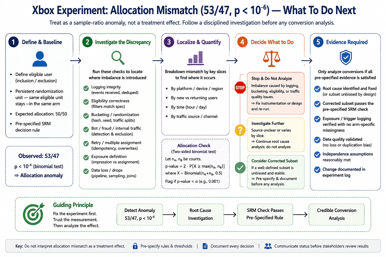
An Xbox checkout experiment expected a 50/50 split but observed 53/47 with p < 10^-6. What should you do next? diagram
How to Explain It in an Interview

Start with the experimental contract. The expected allocation is 50/50 among eligible units. The randomization unit must be persistent: once an eligible unit is assigned, it should remain in the same arm. The observed 53/47 allocation with p < 10^-6 is therefore an allocation anomaly. It is not a treatment-effect result.

Next, investigate where the discrepancy enters the data. Check logging integrity: assignment and exposure events should be received as expected and duplicates should be handled consistently. Check eligibility rules and confirm that filters match the experiment specification. Check bucketing and randomization logic, including the hash, seed or salt, and traffic-split configuration. Check bot, fraud, or internal-traffic handling for arm-specific behavior. Check retries or multiple assignments for overwrites or non-idempotent behavior. Verify the exposure definition so assignment is not confused with an actual impression or trigger. Finally, check data loss, sampling, joins, and pipeline drops for asymmetric missingness.

Then localize the SRM. Break the allocation down by slices such as platform, device, region, new versus returning users, time, and traffic source. The goal is not to hunt for a favorable treatment result. The goal is to find where the allocation mismatch appears and connect that slice to a plausible assignment or data-quality failure.

For a 50/50 design, a two-sided binomial SRM test compares the observed arm counts with the allocation expected under a 0.5 assignment probability. If n_A and n_B are the two arm counts, X follows Binomial(n_A + n_B, 0.5) under the null. The supplied p < 10^-6 already shows that the 53/47 split is highly inconsistent with the intended allocation, so there is no reason to reinterpret that imbalance as a conversion effect.

If logging, eligibility, bucketing, traffic quality, or another experiment mechanism is broken, stop the analysis, correct the problem, and rerun or otherwise obtain trustworthy data. If the source is unclear or changes across slices, continue the root-cause investigation and do not compare conversions.

A corrected subset can be defensible only under a much stronger standard than filtering until the ratio looks balanced. The subset must be well defined, stable, and unbiased with respect to treatment outcomes. Its inclusion or exclusion criteria must be established independently of conversion results and before inspecting treatment-effect outcomes. The corrected subset must pass the pre-specified SRM check. Exposure or trigger logging must show no arm-specific missingness. End-to-end data quality must be validated, relevant independence assumptions must be reasonable, and the correction must be documented in the experiment log.

The final decision is simple: detect the anomaly, identify and resolve the root cause, verify that the SRM check passes the pre-specified rule, and only then trust a conversion comparison. If a corrected subset is used instead of a full rerun, it must satisfy the same pre-specified evidence and data-quality requirements. Fix the experiment first, trust the measurement second, and analyze the treatment effect last.

Technical Approach
  1. Define the eligible population and the persistent randomization unit.
  2. Confirm the intended 50/50 allocation and the pre-specified SRM decision rule.
  3. Treat 53/47 with p < 10^-6 as an SRM and stop treatment-effect interpretation.
  4. Check logging integrity, eligibility rules, bucketing/randomization, bot or internal traffic handling, retries or repeated assignments, exposure definition, and data loss or pipeline drops.
  5. Slice the allocation by platform/device/region, new versus returning users, time, and traffic source to locate where the mismatch appears.
  6. If a mechanism is broken, correct it and obtain trustworthy experimental data before comparing conversions.
  7. If the cause is unclear, continue investigating and do not analyze conversions.
  8. Consider a corrected subset only when it is well defined, stable, unbiased with respect to treatment outcomes, and its criteria were established independently of conversion results before treatment-effect inspection.
  9. Require the corrected subset to pass the pre-specified SRM check, have no arm-specific exposure or trigger missingness, pass end-to-end data-quality checks, satisfy reasonable independence assumptions, and be documented.
  10. Compare conversion only after all required evidence is satisfied.
Practical Insights

The statistical SRM test itself is cheap because it only needs the arm counts. The harder and more expensive work is tracing assignment and event data through eligibility rules, logging systems, bucketing, retries, exposure events, joins, and filters. Slice analysis can increase investigation time because every important segment must be checked consistently. Stopping an experiment or rerunning it costs time and traffic, but that cost is preferable to making a decision from biased data. A corrected subset may save usable observations, but it carries extra bias risk if its rule was chosen after looking at conversion outcomes.

Why Interviewers Ask This

This question tests whether you recognize that trustworthy experimentation comes before treatment-effect estimation. The interviewer wants to see whether you can distinguish a sample-ratio mismatch from a conversion result, define the correct experimental population and persistent randomization unit, investigate common assignment and data-pipeline failures, avoid post-hoc filtering, and state clear evidence requirements before trusting an experiment.

Common interview mistakes

Common mistakes are interpreting the 53/47 imbalance as a treatment effect, comparing conversions before resolving the SRM, assuming a large sample makes the imbalance harmless, checking only the randomization code while ignoring eligibility and logging, confusing assignment with exposure, ignoring retries or duplicated units, filtering users after looking at conversion outcomes, accepting a subset merely because it looks close to 50/50, and rerunning the treatment analysis without documenting the failure and correction.

Interview tip

Lead with the decision: stop treatment-effect analysis because this is an SRM. Then organize your answer as definition, diagnosis, localization, stop-versus-corrected-subset decision, and evidence required before conversion analysis. This shows experimental judgment instead of just listing checks.
Interviewer may ask next
What if the SRM appears only for one platform while every other platform passes the pre-specified allocation check?

I would treat that platform slice as the main clue and investigate what differs there: eligibility, bucketing inputs, app behavior, bot filtering, retries, assignment logging, exposure logging, or pipeline loss. I still would not automatically delete that platform and analyze the rest. A corrected subset is defensible only if the exclusion rule is justified independently of treatment outcomes, is stable and unbiased, was established before conversion-outcome inspection, and the remaining subset passes the pre-specified SRM and data-quality checks. Otherwise I would stop and repair or rerun the experiment.

What if you identify the logging bug after the experiment ends and can reconstruct the missing records?

I would first show that the reconstruction addresses the identified root cause without using treatment outcomes to decide which records to restore. Then I would validate the reconstructed assignment and exposure data end to end, check for arm-specific missingness or duplication, rerun the pre-specified SRM check, confirm reasonable independence assumptions, and document the reconstruction. Only if those checks pass would I trust a conversion comparison on the corrected data. If the reconstruction is incomplete or outcome-dependent, I would not use it for the primary treatment conclusion.

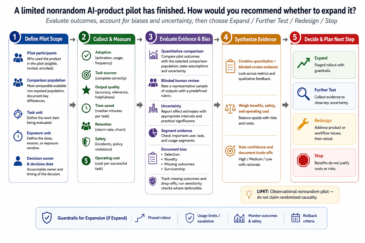
2. A limited nonrandom AI-product pilot has finished. How would you recommend whether to expand it?Model Evaluation And ValidationMediumMicrosoft

Question Details

Define the pilot participants, comparison population, task and exposure units, and the decision owner. Evaluate adoption, task success, output quality, time saved, retention, safety, and operating cost while documenting selection, novelty, missing-outcome, and survivorship biases. Combine quantitative outcomes with blinded human review, uncertainty, and segment evidence, and propose a staged expansion, further test, redesign, or stop decision without claiming randomized causality.

Short Interview Answer (30-60 seconds)

I would treat the pilot as observational evidence, define participants, comparison population, task and exposure units, then assess adoption, task success, quality, time, retention, safety, and cost. I would combine quantitative comparisons with blinded review, uncertainty, segment checks, and bias analysis, then choose staged expansion, further testing, redesign, or stop.

Detailed Explanation

I would evaluate the pilot as a decision problem, not as proof that the AI product caused an outcome. First, I would define who participated, the most comparable available non-exposed population, the work item being evaluated, the exposure window, and the person accountable for the decision. Then I would examine adoption, task success, output quality, time saved, retention, safety, and operating cost. I would combine those measures with blinded human review, uncertainty intervals, segment evidence, and explicit checks for selection, novelty, missing-outcome, and survivorship bias before recommending the next step.

Useful Questions to Ask the Interviewer
  1. Who was eligible for the pilot, who was invited, and who actually participated?
  2. What is the most comparable available non-exposed population, and how different is it from the pilot group?
  3. What should count as one task unit, and what exposure unit or time window represents meaningful product use?
  4. Who owns the expand-or-stop decision, and what business, safety, or cost constraints matter most?
  5. Which outcomes are available for both pilot and comparison populations, and how much outcome data is missing?
  6. Are there user, task, or usage segments where performance or risk is especially important?
A limited nonrandom AI-product pilot has finished. How would you recommend whether to expand it? diagram
How to Explain It in an Interview

I would use five steps that match the decision flow.

  1. Define the pilot scope. I would document the pilot participants, including the eligible, invited, and enrolled groups. I would define the comparison population as the most comparable available non-exposed group and record important differences between the two groups. I would also define the task unit as the work item being evaluated and the exposure unit as the meaningful dose, session, or exposure window. Finally, I would identify the decision owner and when the decision must be made.
  1. Collect and summarize the decision outcomes. I would measure adoption, such as activation, usage, or frequency; task success; output quality, such as accuracy, relevance, and helpfulness where appropriate; time saved per task; retention or continued use; safety events or policy violations; and operating cost, including cost per successful task when that denominator is meaningful. I would not invent a success threshold after seeing the results. The measures should reflect the actual product goal, user benefit, safety, and cost.
  1. Evaluate the evidence and its limitations. For the quantitative comparison, I would compare pilot outcomes with the selected comparison population and state the assumptions behind that comparison. Because assignment was nonrandom, observed differences may reflect who entered the pilot rather than the product itself. I would report effect estimates with appropriate uncertainty intervals and discuss practical significance, not only whether an interval excludes a reference value.

I would add blinded human review for a representative sample of outputs using a predefined rubric. Blinding reduces the chance that reviewers rate an output differently simply because they know which condition produced it. I would also inspect important user, task, and usage segments. A favorable overall average can hide a weak or unsafe result in an important segment.

I would explicitly document four major biases. Selection bias can occur because pilot users differ from nonparticipants. Novelty bias can make early enthusiasm or behavior unrepresentative of longer-term use. Missing-outcome bias appears when failures, rework, or other outcomes are not observed consistently. Survivorship bias appears when analysis overrepresents users who continued while ignoring drop-offs. I would track missing outcomes and drop-offs and run sensitivity analyses where the available data supports them.

  1. Synthesize the evidence. I would combine the quantitative outcomes with blinded-review evidence instead of allowing one attractive metric to dominate the decision. I would weigh user and task benefits against safety risk and operating cost. I would then rate my confidence in the recommendation and document the main tradeoffs and uncertainties. The recommendation should reflect the total evidence, not a single metric.
  1. Choose the next action. If benefits are consistent, safety and cost are acceptable, and the remaining uncertainty is manageable, I would recommend a staged expansion rather than an immediate full rollout. The expansion would use phased rollout, usage limits or escalation paths, monitoring of outcomes and safety, and clear rollback criteria. If important uncertainty remains, I would recommend further testing. If the evidence reveals product or workflow problems, I would redesign and retest. If the benefits do not justify the costs or risks, I would stop.

The central limitation is that this was an observational, nonrandom pilot. I can say that the pilot produced evidence consistent with a benefit or concern, but I should not describe the observed difference as a randomized causal effect. If causal identification becomes important to the decision, the next test should use a stronger design where feasible.

Technical Approach
  1. Define the eligible population, invited and participating users, comparison population, task unit, exposure unit, decision owner, and decision timing.
  2. Validate outcome coverage and summarize adoption, task success, output quality, time saved, retention, safety, and operating cost at the correct unit.
  3. Compare pilot outcomes with the selected comparison population while documenting material baseline differences and assumptions.
  4. Add blinded human review of a representative output sample using a predefined rubric.
  5. Report effect estimates with appropriate uncertainty and discuss practical significance.
  6. Evaluate important user, task, and usage segments rather than relying only on the overall average.
  7. Document selection, novelty, missing-outcome, and survivorship bias; track missing outcomes and drop-offs and run defensible sensitivity checks.
  8. Synthesize quantitative evidence, blinded review, safety, cost, segment results, and uncertainty into an explicit confidence assessment.
  9. Recommend staged expansion, further testing, redesign, or stopping.
  10. If expanding, use phased rollout, usage limits or escalation paths, outcome and safety monitoring, and rollback criteria.
Practical Insights

The main cost is not computational complexity; it is evidence quality and operational effort. A wider comparison across users, tasks, and segments needs more data cleaning and analysis. Blinded human review adds reviewer time and requires a clear rubric. Tracking missing outcomes and drop-offs may require additional instrumentation. Sensitivity analyses add analytical work but show whether the conclusion changes under reasonable assumptions. A staged expansion is slower than an immediate rollout, but it limits risk and creates more evidence. More monitoring and rollback capability also cost engineering and operational effort, but they make expansion safer and more reversible.

Why Interviewers Ask This

This tests whether I can turn imperfect real-world pilot evidence into a defensible product decision. The interviewer wants to see whether I define the evaluation population and units correctly, choose useful outcome measures, recognize bias in a nonrandom pilot, quantify uncertainty, combine quantitative and human-review evidence, examine important segments, and avoid making a causal claim that the study design cannot support. It also tests whether I can translate statistical evidence into a practical expand, test-more, redesign, or stop recommendation with appropriate guardrails.

Common interview mistakes

Common mistakes are treating a nonrandom pilot as if it proved causality; comparing pilot participants with an obviously different population without documenting the differences; leaving task or exposure units undefined; reporting only adoption while ignoring task success, quality, retention, safety, or cost; using only aggregate averages and missing important segments; evaluating output quality without blinded review; reporting point estimates without uncertainty; ignoring users with missing outcomes or users who dropped out; overlooking selection, novelty, and survivorship bias; choosing a success threshold after seeing results; recommending full expansion when a staged rollout would better manage uncertainty; and failing to define monitoring and rollback criteria for an expansion.

Interview tip

Structure the answer as scope, evidence, bias and uncertainty, synthesis, then decision. Say early that the pilot is nonrandom, so you will not claim randomized causality. Finish with explicit conditions for Expand, Further Test, Redesign, and Stop, and mention staged rollout plus rollback if you choose expansion.

Interviewer may ask next
What would you do if the pilot users are much more experienced or motivated than the available comparison population?

I would treat that as a major selection-bias limitation rather than trying to hide it with one adjustment. First, I would document the differences between the groups and compare outcomes within the most comparable user, task, and usage segments available. If defensible, I could use matching or adjustment based on measured pre-pilot characteristics, but I would state that unmeasured differences can still remain. I would run sensitivity checks to see whether reasonable alternative comparison definitions change the conclusion. If the expansion decision depends on a causal estimate and the remaining selection problem is large, I would recommend a stronger follow-up test rather than claiming the pilot proved the product caused the observed improvement.

What if the average outcomes look positive, but one important segment has worse safety or quality results?

I would not recommend unrestricted expansion based on the favorable overall average. I would first verify the segment definition, sample coverage, missing outcomes, and uncertainty to determine whether the issue is credible and practically important. If the risk is real, I would either redesign the product or workflow for that segment, exclude or limit that segment during a staged rollout, or run a targeted follow-up test. Any expansion should include usage limits or escalation paths, monitoring of that segment's outcomes and safety, and rollback criteria. If the safety or quality risk cannot be controlled, I would recommend stopping expansion for that use case.

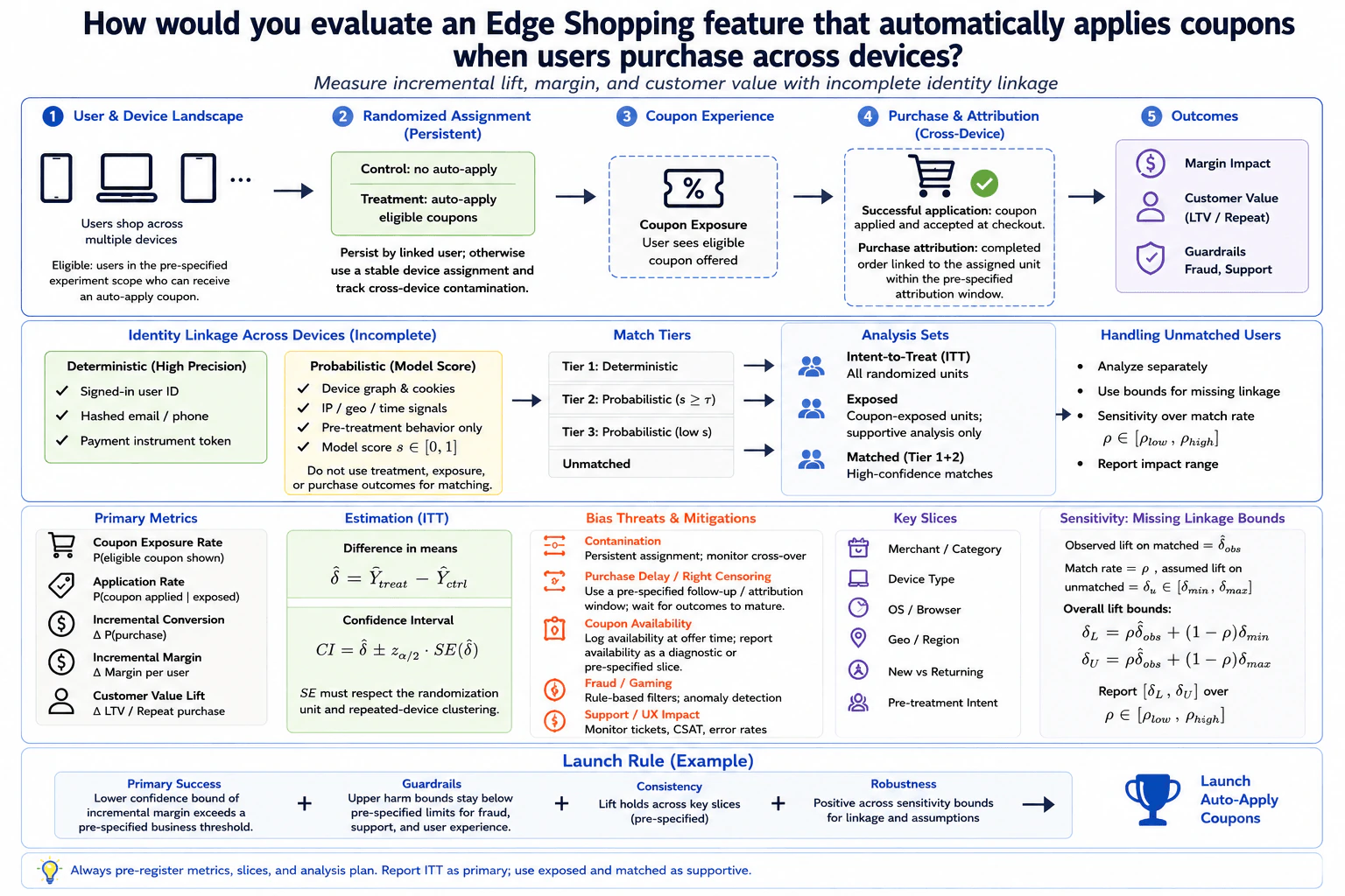
3. How would you evaluate an Edge Shopping feature that automatically applies coupons when users purchase across devices?Model Evaluation And ValidationHardMicrosoft

Question Details

Define eligible users, coupon exposure, successful application, purchase attribution, and margin or customer-value outcomes. Identity linkage across devices is incomplete, so specify deterministic and probabilistic matching, unmatched-user handling, intent-to-treat and exposed analyses, and sensitivity bounds for missing linkage. Cover persistent assignment, contamination, purchase delay, coupon availability, merchant and device slices, fraud, margin and support guardrails, uncertainty, and the launch rule.

Short Interview Answer (30-60 seconds)

I would use persistent randomized assignment and make intent-to-treat the primary analysis. I would define exposure, coupon application, purchase attribution, margin, and customer-value outcomes, then handle incomplete cross-device identity with deterministic and probabilistic matching, unmatched-user sensitivity bounds, confidence intervals, guardrails, and pre-specified launch criteria.

Detailed Explanation

The goal is to estimate whether auto-applying eligible coupons creates incremental customer and business value, not merely whether coupons are used. I would define eligible users before randomization, persist treatment assignment across known linked devices, and track coupon exposure, successful application, purchases, margin, and customer value. Because cross-device identity is incomplete, intent-to-treat is the primary analysis. Deterministic and probabilistic matching support attribution, while unmatched users remain visible through separate reporting and sensitivity bounds. I would also check contamination, delayed purchases, coupon availability, fraud, support impact, uncertainty, and important merchant and device slices before launch.

Useful Questions to Ask the Interviewer
  1. What exactly makes a user eligible for the experiment and for an auto-apply coupon?
  2. What event should count as coupon exposure: availability, display, or an actual offer shown to the user?
  3. What event defines successful application at checkout?
  4. What attribution window should connect a completed purchase back to the assigned experimental unit?
  5. Which business outcome is primary: incremental margin, customer value, conversion, or another pre-specified objective?
  6. Which identity signals are available for deterministic linkage, and what probabilistic linkage score is already supported?
  7. What fraud, support, and user-experience limits must remain below pre-specified harm thresholds?
How would you evaluate an Edge Shopping feature that automatically applies coupons when users purchase across devices? diagram
How to Explain It in an Interview

Start with the experimental unit and assignment. The control group receives no auto-apply behavior, while the treatment group receives auto-application for eligible coupons. Persist assignment by linked user when that identity is known. When it is not, use a stable device assignment and explicitly track cross-device contamination rather than silently changing treatment assignment.

Next, define each event in the funnel. Coupon exposure means the user actually sees an eligible coupon offer. Successful application means the coupon is applied and accepted at checkout. Purchase attribution means a completed order is linked to the assigned experimental unit within the pre-specified attribution window. Business outcomes include incremental conversion, incremental margin per user, and customer-value measures such as repeat purchase or lifetime-value change when the observation horizon supports them. Exposure and application rates are useful diagnostics, but they are not substitutes for the randomized business outcome.

For identity linkage, use deterministic signals first because they are higher precision. The diagram uses signed-in user ID, hashed email or phone, and payment-instrument token. For remaining cases, use a probabilistic match based on device graph and cookies, IP, geography and time signals, and pre-treatment behavior. The linkage model must not use treatment assignment, coupon exposure, or purchase outcomes because those variables can be affected by the experiment and could bias matching. A probabilistic score can create high-confidence matched tiers while leaving uncertain cases unmatched.

Keep intent-to-treat, or ITT, as the primary causal analysis. ITT compares outcomes for all randomized units according to their original assignment, even when exposure or identity linkage is incomplete. This preserves the protection created by randomization. Report exposed users and matched users as supportive analyses only because conditioning on post-assignment exposure or successful linkage can create selection bias.

For the primary ITT estimate, use the treatment-minus-control difference in the chosen outcome, for example δ̂ = Ȳ_treat - Ȳ_ctrl for incremental margin. Report a confidence interval as the estimate plus or minus the chosen critical value times SE(δ̂), consistent with the diagram's CI = δ̂ ± z_(α/2) · SE(δ̂) notation. The standard error must respect the randomization unit and repeated observations from the same user or device rather than pretending every event is independent.

Incomplete linkage needs an explicit sensitivity analysis. Let ρ represent the match rate and δ_obs the observed lift among matched users. Specify a plausible range for the unknown effect among unmatched users, δ_u ∈ [δ_min, δ_max]. Then report overall bounds such as δ_L = ρδ_obs + (1 - ρ)δ_min and δ_U = ρδ_obs + (1 - ρ)δ_max. Vary both the match-rate assumption and the unmatched-user effect assumptions. The point is to show whether the launch conclusion remains positive under plausible missing-linkage scenarios, not to pretend unmatched users are equivalent to matched users.

Then examine the main failure modes. Persistent assignment reduces cross-over, but I would still measure cross-device contamination. Purchases can arrive late, so I would use a pre-specified follow-up and attribution window and wait for outcomes to mature. Coupon availability can differ by merchant or time, so I would log availability at offer time and report it as a diagnostic or pre-specified slice. For fraud or gaming, use pre-specified, treatment-symmetric rules and anomaly checks to flag suspicious behavior and report the resulting guardrail; do not selectively remove observations from one arm after seeing the outcome. Support tickets, customer-satisfaction signals, and error rates are guardrails because a financially positive result can still create a poor user experience.

Slice the results by merchant or category, device type, operating system or browser, geography or region, new versus returning users, and pre-treatment intent. These are diagnostic views, not separate opportunities to redefine success after seeing the data. Pre-specify important slices and interpret them with appropriate uncertainty rather than launching from one favorable subgroup.

The launch rule should also be pre-specified. I would launch only when the lower confidence bound for incremental margin exceeds the business threshold, upper harm bounds remain below the allowed fraud, support, and user-experience limits, lift is reasonably consistent across key pre-specified slices, and the conclusion stays positive across the missing-linkage sensitivity range. I would report ITT as primary and clearly label exposed, matched, unmatched, sensitivity, and diagnostic results as supporting evidence.

Technical Approach
  1. Define the eligible experimental population and the exact events for exposure, successful coupon application, purchase attribution, incremental margin, and customer value.
  2. Randomize control versus auto-apply treatment and persist assignment by linked user; otherwise use stable device assignment and measure cross-device contamination.
  3. Log coupon exposure, application, purchase, availability, fraud, support, and user-experience signals using the pre-specified attribution and follow-up windows.
  4. Link devices deterministically with signed-in user ID, hashed email or phone, or payment-instrument token where available.
  5. For remaining cases, use probabilistic linkage from device graph and cookies, IP, geography and time signals, and pre-treatment behavior only. Do not use treatment, exposure, or purchase outcomes in the matcher.
  6. Keep uncertain identities unmatched instead of forcing a link. Report deterministic, probabilistic, matched, and unmatched populations separately.
  7. Estimate the primary intent-to-treat treatment effect across all randomized units. Use exposed and matched analyses only as supportive views.
  8. Report uncertainty with confidence intervals whose standard errors respect the assignment unit and repeated observations from a user or device.
  9. Compute sensitivity bounds for missing linkage by varying the match rate and the assumed effect among unmatched users.
  10. Diagnose merchant or category, device type, OS or browser, geography, new versus returning, and pre-treatment-intent slices.
  11. Check contamination, purchase delay, coupon availability, fraud or gaming, support, and user-experience guardrails using pre-specified, treatment-symmetric rules.
  12. Launch only if the pre-specified primary margin criterion, harm bounds, slice consistency, and linkage-sensitivity requirements all pass.
Practical Insights

The main difficulty is not computational complexity; it is getting an unbiased causal estimate from imperfect identity data. Deterministic links are easier to trust but leave more users unmatched. Probabilistic matching increases coverage but adds model uncertainty and possible false links. Keeping unmatched users separate is safer, but it widens the uncertainty range. ITT is robust because it keeps the original randomization, while exposed or matched-only analyses can look more targeted but are more vulnerable to selection bias. Longer purchase windows capture delayed orders but make experiments take longer. More merchant and device slices help find failures, but they also increase statistical uncertainty and the risk of chasing noisy subgroup results. Operationally, the experiment also needs persistent assignment, reliable cross-device logging, availability records, fraud checks, and support monitoring.

Why Interviewers Ask This

This question tests whether I can design a trustworthy randomized evaluation when the same user shops on multiple devices and identity linkage is incomplete. The interviewer wants to see whether I can define the experimental population and outcomes, keep assignment persistent, separate intent-to-treat from post-assignment analyses, handle missing linkage without hiding uncertainty, choose business and guardrail metrics, diagnose important slices, and translate statistical evidence into a defensible launch decision.

Common interview mistakes

Common mistakes are using coupon application rate as the main success metric instead of incremental business value; changing treatment assignment when a user switches devices; forcing uncertain devices into a matched identity; using treatment, exposure, or purchase outcomes as inputs to the identity matcher; analyzing only exposed or matched users and calling that the randomized effect; dropping unmatched users without sensitivity bounds; ignoring delayed purchases or right censoring; conditioning the primary causal estimate on coupon availability after randomization; using post-outcome or treatment-asymmetric fraud exclusions; overlooking cross-device contamination; reporting many merchant or device slices without pre-specification; ignoring fraud, support, or user-experience harm; and launching from a point estimate without confidence intervals, practical thresholds, or robustness to missing linkage.

Interview tip

Organize the answer around four ideas: persistent randomization, identity uncertainty, ITT as the primary causal estimate, and a pre-specified launch rule. Explicitly say that matched and exposed analyses are supportive, not replacements for ITT, and explain how sensitivity bounds keep unmatched users from disappearing from the decision.

Interviewer may ask next
What would you do if probabilistic identity matching covers many additional purchases but you are not confident that the matches are correct?

I would not force those matches into the primary estimate. The ITT analysis would remain based on original randomization. I would keep deterministic links as the highest-confidence tier, define a pre-specified probabilistic-score threshold for supportive matched analysis, and leave low-confidence cases unmatched. I would then vary both the assumed match rate and the possible outcome effect among unmatched users to produce sensitivity bounds. If the launch conclusion changes materially when plausible matching assumptions change, I would treat identity uncertainty as unresolved rather than reporting a single precise effect.

How would your decision change if the point estimate for incremental margin is positive but the result is weak in some devices or under the missing-linkage sensitivity analysis?

I would not launch solely from the positive point estimate. I would first check whether the lower confidence bound clears the pre-specified business threshold and whether fraud, support, and user-experience harm bounds remain acceptable. I would examine the pre-specified device slices to determine whether the weakness is consistent or just noisy, and I would test whether the overall conclusion stays positive across plausible linkage assumptions. If the decision becomes negative under reasonable sensitivity bounds or shows a material failure in a key slice, the launch rule has not passed.

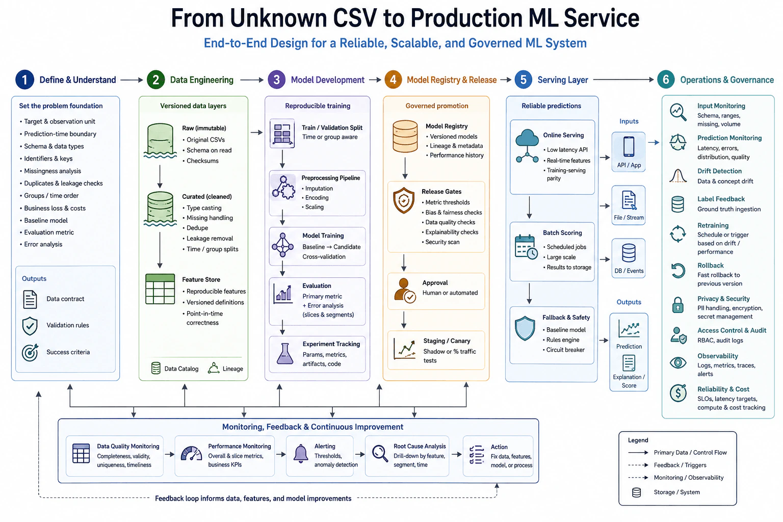
4. Turn a baseline model built from an unknown CSV into a production machine-learning service.Machine Learning System DesignEasyMicrosoft

Question Details

Start by defining the target, observation unit, prediction-time boundary, schema, identifiers, missingness, duplicate and leakage checks, groups or time order, business loss, baseline, metric, and error analysis. Then design versioned raw and curated datasets, reproducible preprocessing and feature definitions, training and validation, experiment tracking, model registry and release gates, online or batch serving with training-serving parity and fallback, input and prediction monitoring, label feedback, drift detection, retraining and rollback, privacy and secret handling, access controls, failure recovery, observability, and latency and compute cost.

Short Interview Answer (30-60 seconds)

I would first define the prediction contract and audit the unknown CSV. Then I would build versioned raw and curated data, reproducible preprocessing, time- or group-aware validation, experiment tracking and release gates. I would serve the approved model online or in batch with fallback, monitoring, label feedback, retraining, and rollback.

Detailed Explanation

Turning an unknown CSV and a baseline model into a production service starts with defining what a prediction means before building more infrastructure. I would establish the target, observation unit, prediction-time boundary, identifiers, schema, business loss, baseline, and evaluation metric, then inspect missing values, duplicates, leakage, groups, and time ordering. From there I would build versioned raw and curated data, reproducible features and training, controlled model promotion, reliable online or batch inference, monitoring, feedback, retraining, and rollback while treating security, observability, latency, reliability, and cost as system requirements.

Useful Questions to Ask the Interviewer
  1. What exactly is the target, and what real-world decision will use the prediction?
  2. What is one observation or prediction unit, and which identifiers uniquely represent it?
  3. At what moment must the prediction be made, and which data is guaranteed to exist by that moment?
  4. Are observations independent, grouped by an entity, ordered in time, or both?
  5. What business cost do false positives and false negatives create, and which evaluation metric should reflect that cost?
  6. Is the prediction needed synchronously through an online API, asynchronously from a stream, periodically through batch scoring, or should the design support more than one path?
  7. What latency, throughput, freshness, availability, and compute-cost constraints apply?
  8. When do ground-truth labels become available, and how can they be joined back to the correct prediction?
  9. What privacy, retention, access-control, and secret-handling requirements apply to the data and service?
Turn a baseline model built from an unknown CSV into a production machine-learning service. diagram
How to Explain It in an Interview

I would organize the design into six connected stages plus a continuous feedback loop.

1. Define the prediction contract and inspect the CSV

Before changing the baseline, I would define the target and the observation unit. The observation unit is the thing represented by one prediction. Because the CSV is unknown, I would not assume whether that unit is a user, transaction, device, or another entity.

I would also establish the prediction-time boundary. This is the point in time when the system must produce the prediction. A feature is valid only if it would have been available by that boundary. This prevents future information from leaking into training.

Next I would inspect the schema and data types, identify stable IDs or keys, profile missingness, detect duplicate observations, and look for direct or indirect target leakage. If rows belong to the same entity or have a meaningful time order, that structure must be preserved when splitting data.

I would connect the model objective to the business objective by defining the cost of important mistakes, keeping the existing baseline as the comparison point, choosing an evaluation metric that reflects the decision, and performing error analysis across relevant slices. The output of this stage is a clear data contract, validation rules, and success criteria rather than assumptions hidden inside a notebook.

2. Build versioned data foundations

I would keep an immutable version of the original CSV as the raw dataset. Each ingestion should be traceable with metadata such as the data version, schema, and integrity information. I would then create a curated dataset after applying deterministic cleaning rules such as type handling, missing-value treatment, deduplication, and leakage-safe filtering.

Raw and curated data should be separately versioned so a training run can be reproduced. Schema and data-quality checks should fail early when required fields disappear, types change unexpectedly, values become invalid, or duplicate behavior violates the contract.

If time or groups matter, the curated data must retain enough identifiers and timestamps to construct valid training and validation sets. Point-in-time correctness means that a historical training example receives only features that existed before its prediction boundary.

3. Make preprocessing, features, training, and validation reproducible

Preprocessing should be represented as a reproducible pipeline rather than manually prepared columns. Imputation, encoding, scaling, and feature transformations must be fit using the training portion where required and then applied consistently to validation and serving data.

Feature definitions should be versioned with the code and configuration that produces them. If a feature store or equivalent reusable feature layer is useful, it can hold those definitions and help maintain point-in-time correctness and training-serving parity. The important principle is not the product name; it is that training and inference compute the same feature meaning from the same definition.

I would compare the baseline with candidate models using a split strategy appropriate to the data. Random splitting is acceptable only when observations are independent and time does not create leakage. Group-aware validation keeps related observations together. Time-aware validation trains on the past and evaluates on later data. Cross-validation may be used when it is compatible with those constraints.

Evaluation would use the agreed primary metric plus error analysis across meaningful slices. I would not promote a model just because its training score improved. Every run should record parameters, code or configuration version, data version, feature definitions, metrics, and produced artifacts so the result can be reproduced and investigated later.

4. Register the candidate and apply release gates

A candidate that passes evaluation becomes a versioned model artifact in a model registry together with lineage, experiment metadata, and evaluation history. The registry gives each releasable model a clear identity and keeps previous known-good versions available for rollback.

Promotion should pass explicit release gates. Relevant gates include performance against the baseline, data-quality checks, robustness checks, security review, explainability checks when needed, and bias or fairness checks when those concerns apply to the prediction context. Approval may be automated or require a human depending on risk.

I would first expose a newly approved version in a controlled environment, such as staging, shadow traffic, or a small canary percentage when online serving is used. Promotion occurs only after the release evidence is acceptable. Otherwise the candidate remains unpromoted or is rolled back.

5. Serve through the path that matches the requirement

Offline training, online serving, streaming inference, and batch inference are different execution paths.

Offline training reads historical versioned data and produces a validated model artifact. It is not part of the request-time prediction path.

For online serving, an application sends a synchronous request to an API. The service validates the request contract, obtains or computes the same feature meanings used during training, scores the approved model, and returns a prediction. Request IDs and model-version metadata should make the prediction traceable. I would measure end-to-end request latency separately from model execution time because serialization, feature retrieval, network calls, queues, and other service work can dominate total latency.

Streaming inference is appropriate when records arrive continuously but do not require a synchronous request-response API. Each event is validated, transformed with the same versioned feature logic, scored, and written to a downstream event or data system while retaining the entity, event time, prediction time, and model version needed for later feedback.

For batch inference, a scheduled job reads a defined input snapshot or partition, applies the same preprocessing and feature definitions, performs large-scale scoring, and writes predictions to traceable storage. Batch processing is often simpler and less expensive when immediate responses are unnecessary.

Training-serving parity is a central requirement in every inference path. Preprocessing and feature semantics must not silently differ between offline training and production inference.

I would also provide safe degradation. If the active model is unavailable, required features are stale or missing, the service times out, or load exceeds safe capacity, the system should follow an explicitly defined fallback such as a previous known-good model or rules-based behavior. A circuit breaker or equivalent protective mechanism can stop repeated calls to a failing dependency. The exact fallback depends on the product requirement and should not be invented before that requirement is known.

6. Monitor the system and close the feedback loop

Monitoring should separate different kinds of signals instead of treating them as one health score.

Service monitoring covers latency, errors, timeouts, saturation, availability, and resource use. Data-quality monitoring covers schema, missingness, validity, uniqueness, and freshness. Prediction monitoring covers output distributions and relevant model-output behavior. Drift monitoring can detect changes in features, predictions, or relationships, but drift alone does not prove that predictive quality has declined. Fairness monitoring, when relevant to the use case, should be evaluated separately rather than inferred from general drift. Business outcomes should also be tracked separately from technical service health.

True model-quality measurement requires outcomes. When labels arrive, I would join each delayed outcome back to the original prediction using the correct entity identifier and prediction time. The stored prediction record should retain the request or event identifier, feature or feature-version reference, model version, prediction, and timestamp needed for that join. This produces a labeled evaluation dataset at the same grain as the original prediction contract. I would then measure the primary metric and relevant slice metrics over time.

Retraining should be triggered by evidence rather than blindly by every drift alert. Possible triggers include an agreed schedule, enough new labeled data, validated performance degradation, or another explicitly defined operational condition. A retrained challenger must pass the same validation and release gates as the original model.

Rollback should be fast because model and preprocessing artifacts are versioned. If a deployment degrades service health or validated model quality, traffic can return to the previous known-good version while the issue is investigated.

Cross-cutting production requirements

Privacy and security apply across the pipeline. Sensitive data should be minimized, protected according to the required policy, and never embedded in source code or model configuration as secrets. Secrets belong in a managed secret mechanism, and access should follow least privilege with auditable permissions.

Failure recovery should cover retries where operations are safe to retry, idempotent jobs where repeated execution must not duplicate results, checkpoints or durable state where needed, and recovery procedures for unavailable models or data dependencies.

Observability should connect logs, metrics, traces, alerts, model versions, request identifiers, and data lineage so an incident can be traced from a bad prediction or failed request back through the serving and training artifacts.

Finally, latency and compute cost influence architecture. Online inference offers immediate responses but usually requires continuously available serving capacity and stricter latency engineering. Streaming inference can provide fresher asynchronous predictions than periodic batch jobs but adds event-processing and operational complexity. Batch inference can process work efficiently on a schedule but produces less-fresh predictions. Model complexity, feature computation, storage, retraining frequency, and monitoring all have ongoing cost. I would choose the simplest architecture that meets the clarified product requirements rather than assuming the most complex production stack.

Technical Approach
  1. Define the target, observation unit, prediction-time boundary, identifiers, business loss, baseline, metric, and success criteria.
  2. Profile the unknown CSV for schema, types, missingness, duplicates, leakage, groups, and time ordering.
  3. Store the original data as an immutable versioned raw dataset and create a deterministic versioned curated dataset with validation rules.
  4. Build reproducible preprocessing and versioned feature definitions with point-in-time correctness where time matters.
  5. Train baseline and candidate models using random, group-aware, or time-aware validation according to the data structure.
  6. Record parameters, code or configuration, data versions, feature definitions, metrics, and artifacts for every experiment.
  7. Register acceptable candidates and apply release gates based on validation evidence rather than training performance alone.
  8. Release through staging, shadowing, or canary exposure when appropriate.
  9. Select online serving, streaming inference, or scheduled batch scoring according to latency, freshness, and interaction requirements while preserving training-serving parity.
  10. Make requests, events, predictions, model versions, and delayed outcomes traceable at the correct entity and time.
  11. Define fallback behavior for missing models, invalid inputs, stale features, timeouts, and overload according to product requirements.
  12. Monitor service health, input quality, prediction behavior, drift, model quality, fairness when relevant, and business outcomes as separate signals.
  13. Join delayed labels to predictions at the correct entity and time, retrain when justified, revalidate the challenger, promote only after gates pass, and retain a fast rollback path.
Practical Complexity & Trade-offs

The biggest tradeoff is usually not algorithmic Big-O complexity but operational complexity. More features, larger models, and more frequent retraining can increase training time, inference time, storage, and compute cost. Online serving adds strict latency and availability requirements. Streaming inference gives fresher asynchronous predictions but requires event-processing infrastructure and careful handling of ordering, retries, and duplicate events. Batch scoring is usually operationally simpler but gives less-fresh predictions. A feature store or similar reusable feature layer can reduce duplicated feature logic and training-serving skew, but it introduces infrastructure and maintenance cost. Strong versioning, experiment tracking, validation gates, monitoring, and rollback also add engineering work, but they reduce the cost of reproducing failures and recovering from bad releases. The design should therefore use only the components needed to satisfy the actual latency, freshness, reliability, privacy, and cost requirements.

Where it is used

This approach is useful whenever an exploratory or notebook-based model must become a repeatable production capability. It fits tabular prediction problems where source data arrives as files, tables, or streams and the team needs controlled training, reproducible features, model release management, synchronous API predictions, asynchronous streaming predictions, or scheduled batch scores, plus operational monitoring, delayed-label evaluation, and safe retraining. It is especially useful when duplicate entities, grouped observations, time ordering, leakage risk, changing input distributions, privacy controls, or production reliability make a simple model script insufficient.

Why Interviewers Ask This

This question tests whether a candidate can turn an exploratory model into a reliable end-to-end system rather than treating model training as the whole solution. The interviewer is looking for judgment around defining the prediction problem, preventing leakage, creating reproducible data and features, validating against a baseline, controlling model promotion, choosing online, streaming, or batch inference appropriately, preserving training-serving parity, handling failures safely, and closing the loop with monitoring, labels, drift analysis, retraining, rollback, security, observability, latency, and cost.

Common interview mistakes

Common mistakes are choosing a target or prediction unit without confirming the business decision; randomly splitting time-ordered or grouped data; allowing future information into features; removing duplicates without understanding their entity meaning; fitting preprocessing on the full dataset; manually recreating feature logic in production; evaluating only a training metric; failing to version raw data, curated data, features, code, configuration, models, and evaluation artifacts; promoting a model without explicit validation gates; drawing online, streaming, and batch inference as if every prediction goes through all of them; measuring only model execution time while ignoring end-to-end latency; having no behavior for stale features, missing models, invalid requests, timeouts, or overload; interpreting drift as proof of quality loss; collecting labels without joining them to the original prediction at the correct entity and time; automatically retraining and deploying on every alert; mixing service health, data quality, drift, model quality, fairness, and business outcomes into one metric; storing secrets in code; giving broad access to sensitive data; and lacking a tested rollback path to a previous known-good version.

Interview tip

Start with the prediction contract, not infrastructure. Then walk left to right through versioned data, reproducible training, release gates, serving, and the feedback loop. Explicitly distinguish offline training, online serving, streaming inference, and batch scoring, and distinguish drift from measured quality loss. Finish with fallback, rollback, security, observability, latency, and cost.

Interviewer may ask next
What would you change if the CSV contains many rows from the same entity or records that are ordered in time?

I would first identify the stable entity key and the relevant timestamps. If multiple rows belong to the same entity, I would keep related observations together when splitting so the same entity does not leak information across training and validation. If time determines what information was available, I would use time-aware validation, training on earlier observations and evaluating on later ones. Feature generation would also follow the prediction-time boundary so each historical row receives only information that existed at that time. The raw and curated datasets would retain the identifiers and timestamps needed to reproduce those splits and point-in-time features. I would apply the same rules to the baseline and every candidate so their comparison remains fair.

What would you do if production drift monitoring fires but labeled outcomes will not arrive for several weeks?

I would treat the drift alert as evidence that the input or prediction distribution changed, not as proof that model quality declined. I would inspect which features or prediction slices moved, check data-quality and service-health signals, and determine whether the change is caused by a pipeline problem, a real population change, or another known event. Until labels arrive, I would avoid automatically promoting a retrained model solely because of drift. If the change creates a safety or reliability concern, I could use the defined fallback or roll back to a known-good version. When outcomes arrive, I would join them to the original predictions by identifier and prediction time, measure the agreed quality metrics, and use that evidence to decide whether retraining and a new gated release are justified.

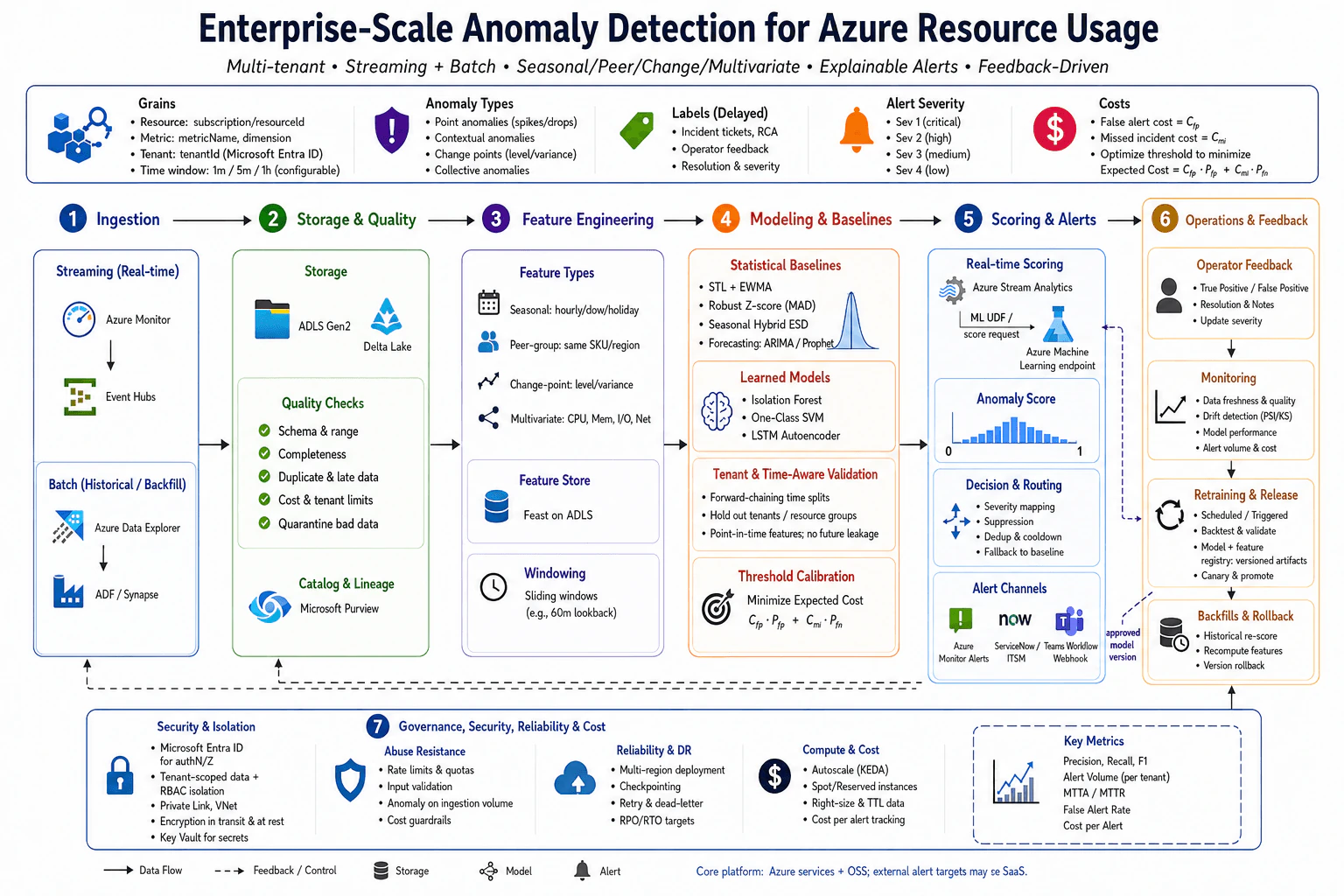
5. Design an enterprise-scale anomaly-detection system for Azure resource usage.Machine Learning System DesignMediumMicrosoft

Question Details

Define the resource, metric, tenant and time-window grains; anomaly types; delayed incident or operator labels; alert severity; and false-alert and missed-incident costs. Design streaming and batch ingestion, schema and quality checks, seasonal, peer-group, change-point and multivariate features, statistical and learned baselines, tenant and time-aware validation, threshold calibration, model and feature registry, low-latency scoring and alert routing with suppression and fallback, operator feedback, drift and alert-volume monitoring, retraining, backfills and rollback, tenant isolation, encryption, access control, abuse resistance, disaster recovery, and compute and on-call cost.

Short Interview Answer (30-60 seconds)

I would combine streaming Azure Monitor data and historical backfills, build seasonal, peer, change-point, and multivariate features, validate across time and tenants, calibrate thresholds by alert cost, score through Azure Machine Learning, suppress noisy alerts, and close the loop with operator feedback, monitoring, retraining, backfills, and rollback.

Detailed Explanation

The system should detect unusual Azure resource usage without creating an unmanageable alert burden. I would define each observation by tenant, resource, metric, and time window, with configurable windows such as 1 minute, 5 minutes, and 1 hour. Streaming data supports fast detection, while historical batch data supports training and backfills. Because incident and operator labels arrive later, features and validation must respect event time and prevent future information from leaking backward. The final alert decision should combine calibrated anomaly scores, severity, suppression, and the relative cost of false alerts versus missed incidents.

Useful Questions to Ask the Interviewer
  1. Which Azure resources and metrics are in scope, and should the same model cover every resource type or can models differ by tenant, resource class, or metric?
  2. What time windows matter operationally, such as 1 minute, 5 minutes, 1 hour, or another configurable set?
  3. What anomaly types matter most: spikes and drops, contextual seasonal anomalies, peer deviations, level shifts, variance changes, or multivariate behavior?
  4. How are incident tickets and operator decisions recorded, and how long after the original metric event do those labels normally become available?
  5. How should alert severity be mapped, and how much more expensive is a missed incident than a false alert?
  6. What end-to-end alert latency is required, and how stale can a metric or feature become before scoring should degrade or stop?
  7. Are there tenant-specific isolation, access-control, retention, encryption, or regional requirements?
  8. What alert destinations are required, such as Azure Monitor Alerts, ServiceNow or another ITSM system, and Microsoft Teams workflows or webhooks?
  9. What operational limits matter most: compute budget, alert volume per tenant, storage growth, or on-call workload?
Design an enterprise-scale anomaly-detection system for Azure resource usage. diagram
How to Explain It in an Interview
1. Define the prediction grain and decision

I would first make the data contract explicit. One scoring record represents one tenant, one Azure resource, one metric or metric dimension, and one configured time window. The diagram uses windows such as 1 minute, 5 minutes, and 1 hour, but they are configurable rather than hard service guarantees.

The system produces an anomaly score and then decides whether to create an alert and what severity to assign. Severity is mapped into levels such as Sev 1 through Sev 4. The threshold is not chosen only to maximize a model metric. It is calibrated using the operational cost of false positives and false negatives, where a false positive creates unnecessary engineer or on-call work and a false negative can miss a real incident.

A useful objective is to choose the threshold that minimizes expected cost:

Expected cost = C_fp * P_fp + C_mi * P_fn

Here C_fp is the cost of a false alert, C_mi is the cost of a missed incident, P_fp is the probability of a false positive under the chosen threshold, and P_fn is the probability of a false negative.

2. Ingest both real-time and historical data

For the streaming path, configured Azure Monitor telemetry is exported to Event Hubs. This path feeds the low-latency feature and scoring workflow.

For historical processing, the design uses Azure Data Explorer together with ADF or Synapse orchestration for history and backfills. Governed historical records are retained in ADLS Gen2 with Delta Lake so training, validation, feature recomputation, and replay can work from durable historical data rather than from the live stream alone.

Streaming inference and batch processing stay logically separate. Streaming is optimized for fast scoring. Batch processing is optimized for larger historical scans, training, validation, backfills, and historical rescoring.

3. Enforce schema and data-quality contracts

Before modeling, I would validate schema, expected ranges, completeness, duplicate records, late data, tenant limits, and cost limits. Invalid data is quarantined rather than silently entering training or serving.

The key identifiers and timestamps must be stable so that the same tenant, resource, metric, and time window are not counted twice. Late events should be handled according to event time, not merely arrival time. Catalog and lineage information can be maintained with Microsoft Purview so data and downstream artifacts can be traced.

4. Build features that match the anomaly types

I would use several complementary feature families because no single detector handles every anomaly type well.

Seasonal features capture expected hourly, day-of-week, or holiday patterns. Rolling statistics and decomposition can represent recurring behavior.

Peer-group features compare a resource with similar resources, such as the same SKU or region. This catches a resource that looks normal in isolation but abnormal relative to comparable resources.

Change-point features capture level or variance changes. They are useful when behavior shifts and stays shifted rather than creating only a single spike.

Multivariate features combine related signals such as CPU, memory, I/O, and network activity. They can expose anomalies that are not obvious in any single metric.

The diagram uses a feature store implemented with Feast on ADLS and a sliding-window representation such as a 60-minute lookback. The important production requirement is that training and serving use the same feature definitions and only information that was actually available at the scoring time.

5. Prevent leakage with point-in-time feature construction

For every historical training row, features must be reconstructed as they would have existed at that event time. A feature produced after the scoring timestamp cannot be joined backward into that example.

This is especially important because incident tickets, resolution notes, and operator feedback are delayed outcomes. They may be used as labels after they arrive, but they must never appear inside features for an earlier prediction.

Point-in-time correctness also prevents a historical backfill from accidentally using a newer feature state than the model would have seen online.

6. Use both statistical and learned baselines

I would keep statistical baselines because they are inexpensive, interpretable, and useful for fallback. The diagram includes STL plus EWMA, robust Z-scores using MAD, Seasonal Hybrid ESD, and forecasting approaches such as ARIMA or Prophet.

I would also evaluate learned anomaly models such as Isolation Forest, One-Class SVM, and an LSTM autoencoder. Learned models may capture nonlinear or multivariate behavior, but they add training, serving, tuning, and monitoring cost.

The production choice does not have to be one model for every tenant. A tenant or resource may use a more specific model when enough representative history exists and fall back to a broader statistical or peer-based baseline when it does not.

7. Validate across time and tenants

Random train-test splitting is unsafe for this problem because it mixes future and past behavior. I would use forward-chaining time splits so validation always predicts later periods from earlier information.

I would also hold out tenants or resource groups when appropriate. This tests whether a model is learning a generally useful anomaly pattern rather than memorizing one tenant's behavior.

The validation gate should check both detection quality and operational behavior. Useful metrics include precision, recall, F1, false-alert rate, alert volume per tenant, and cost per alert. Because labels are delayed, evaluation should be recomputed as outcomes mature rather than treating unlabeled recent predictions as known negatives.

8. Calibrate thresholds by operational cost

The anomaly model produces a score; the alert policy converts that score into an operational decision. I would calibrate thresholds on time-aware validation data and consider separate thresholds where tenant or resource behavior genuinely differs.

The main tradeoff is false alerts versus missed incidents. Lower thresholds catch more anomalies but increase noise and on-call cost. Higher thresholds reduce noise but increase the risk of missed incidents.

Threshold calibration therefore belongs after model scoring, not inside the training metric alone. Severity mapping can also consider the anomaly score and supported operational context rather than treating every anomaly as equally urgent.

9. Version models, features, and release artifacts

A production release should identify the exact model version, feature definitions, training data lineage, configuration, threshold configuration, code version, and validation results used to approve it. The diagram represents this with a versioned model and feature registry.

A candidate is promoted only after backtesting and validation. The release path can use canary promotion before broader rollout. This keeps deployment separate from training and gives the team a controlled rollback point.

10. Serve the approved model with a low-latency path

For real-time scoring, Azure Stream Analytics receives streaming measurements and sends a score request through an ML UDF to an Azure Machine Learning endpoint. The endpoint returns an anomaly score.

It is important to distinguish model execution time from end-to-end alert latency. The latter includes ingestion delay, feature calculation, network calls, model scoring, thresholding, suppression, routing, and the destination system.

If the endpoint times out, a feature is stale, or an approved model is unavailable, the system should degrade safely. The diagram uses a baseline fallback rather than simply dropping detection. A simpler statistical baseline can continue producing conservative anomaly decisions until the learned endpoint recovers.

11. Route alerts without overwhelming operators

The anomaly score flows into decision and routing logic. That layer maps severity, applies suppression, performs deduplication and cooldown, and invokes fallback behavior when required.

Suppression is important because one root cause can create repeated anomalous observations. Deduplication and cooldown reduce multiple pages for the same continuing event. Alert volume should also be monitored per tenant so one noisy tenant cannot dominate the operational channel.

The diagram routes alerts to Azure Monitor Alerts, ServiceNow or another ITSM destination, and a Microsoft Teams workflow or webhook destination. These are operational targets; they are separate from model execution.

12. Join delayed operator feedback to the original prediction

Operators can confirm true positives or false positives, add resolution notes, and update severity. That feedback must be joined back to the original prediction using the same tenant, resource, metric, and event-time identity.

The label time is different from the event time. A prediction can occur immediately while an incident ticket or operator resolution may arrive much later. Training data should therefore retain both when the metric event happened and when the outcome became known.

This delayed-feedback design avoids falsely labeling recent alerts as negatives merely because nobody has resolved them yet.

13. Monitor different kinds of failure separately

I would not use one generic health metric. Data freshness and quality, service health, drift, model quality, alert volume, and operational cost answer different questions.

The diagram monitors data freshness and quality, drift with statistics such as PSI or KS where appropriate, model performance once labels mature, alert volume, and cost. Drift is evidence that the input distribution changed; it is not proof that model quality declined. A drift alarm should trigger investigation or evaluation rather than automatically forcing retraining.

The serving path should separately monitor timeouts, endpoint errors, stale features, missing approved model versions, processing lag, and fallback usage.

14. Retrain, backfill, and roll back safely

Retraining can be scheduled or triggered by evidence such as enough new labeled data, material drift together with quality degradation, or changed resource behavior. New candidates are backtested and validated before promotion.

Backfills recompute historical features or rescore historical data when needed. They must use versioned feature definitions and point-in-time rules so they do not rewrite history with information that was unavailable at the original prediction time.

If a newly promoted model or threshold behaves badly, versioned artifacts allow rollback to the prior approved model and configuration. Historical rescoring can then quantify what changed.

15. Protect tenants and control abuse

Tenant identity is represented through Microsoft Entra ID. Tenant isolation should exist in the data model and access path, not only in an application filter. Data should be tenant-scoped, with RBAC enforcing authorized access.

The design also includes Private Link or VNet controls where appropriate, encryption in transit and at rest, and Key Vault for secrets. Rate limits, quotas, input validation, and monitoring of unusual ingestion volume reduce the risk that one tenant or malformed input overwhelms the shared platform.

The same tenant boundary must be respected in storage, feature access, model access, alert routing, feedback, and monitoring.

16. Design for reliability and disaster recovery

The platform should use checkpointing, retry, and dead-letter handling so transient failures do not silently lose events. A multi-region strategy can support disaster recovery according to required RPO and RTO targets, but I would ask the interviewer for those target values instead of inventing them.

A degraded scoring mode is valuable during partial failure. If the learned Azure Machine Learning endpoint is unavailable, a simpler statistical baseline can continue producing conservative detections. The system should record when fallback was used so later evaluation does not mix primary-model predictions with fallback predictions without distinction.

17. Control compute and on-call cost

Cost comes from more than model inference. Streaming compute, historical scans, feature storage, retention, endpoint capacity, retraining, backfills, alert delivery, and operator time all matter.

The diagram uses autoscaling with KEDA where appropriate, spot or reserved capacity where suitable, right-sized and tiered data retention, and cost-per-alert tracking. I would also control expensive feature calculations and bound per-tenant ingestion or alert volume.

A more sophisticated model is not automatically better if it slightly improves detection but dramatically increases serving cost, maintenance cost, or on-call noise.

18. Final decision

The final architecture is a closed loop. Azure resource data enters through streaming and batch paths, passes quality checks, becomes point-in-time seasonal, peer, change-point, and multivariate features, and is scored by validated statistical or learned models. Calibrated thresholds convert scores into severity-aware alerts with suppression and fallback. Operators provide delayed outcomes, which feed monitoring, evaluation, retraining, backfills, and controlled releases. Versioning, tenant isolation, access control, encryption, reliability mechanisms, disaster-recovery planning, and cost monitoring make the design suitable for an enterprise multi-tenant environment.

Technical Approach
  1. Define the observation contract as tenant, resource, metric or dimension, event time, and configurable time window.
  2. Define anomaly types, severity levels, delayed label semantics, and false-alert versus missed-incident cost.
  3. Ingest configured Azure Monitor telemetry through Event Hubs and maintain a separate historical batch and backfill path.
  4. Use Azure Data Explorer with ADF or Synapse orchestration for historical processing, and retain governed history in ADLS Gen2 with Delta Lake.
  5. Validate schema, range, completeness, duplicate and late events, tenant limits, and bad-data quarantine; maintain catalog and lineage with Microsoft Purview.
  6. Build seasonal, peer-group, change-point, and multivariate features with point-in-time correctness; use the Feast-on-ADLS feature-store path shown in the diagram.
  7. Evaluate statistical baselines such as STL plus EWMA, robust Z-score, Seasonal Hybrid ESD, and forecasting together with learned models such as Isolation Forest, One-Class SVM, and LSTM autoencoders.
  8. Validate with forward-chaining time splits and tenant or resource-group holdouts; reject candidates with leakage or unacceptable operational behavior.
  9. Calibrate anomaly-score thresholds against false-alert and missed-incident cost and map accepted alerts to severity.
  10. Version model, feature, data, configuration, threshold, code, and evaluation artifacts; backtest and validate before canary promotion.
  11. Score streaming events through Azure Stream Analytics and an Azure Machine Learning endpoint using the ML UDF score-request path; measure full end-to-end latency, not only model execution time.
  12. Apply severity mapping, suppression, deduplication, cooldown, and a statistical-baseline fallback when the learned path is unavailable.
  13. Route alerts to Azure Monitor Alerts, ITSM systems such as ServiceNow, and Microsoft Teams workflow or webhook destinations.
  14. Join operator true-positive or false-positive decisions, resolution notes, and severity updates back to the original prediction at the correct tenant, resource, metric, and event time.
  15. Monitor data freshness and quality, service health, drift, mature-label model quality, alert volume, fallback usage, and cost separately.
  16. Retrain only after sufficient evidence, validate the candidate again, backfill with point-in-time rules, and retain version rollback.
  17. Enforce Microsoft Entra ID authentication, tenant-scoped data, RBAC, network controls, encryption, secrets management, rate limits, quotas, and input validation.
  18. Use checkpointing, retry, dead-letter handling, multi-region disaster-recovery planning, autoscaling, right-sized retention, and cost-per-alert tracking.
Practical Complexity & Trade-offs

The main cost is not a single Big-O term because this is a distributed ML system. Streaming work grows roughly with the number of incoming metric events and the number of features computed for each event. Multivariate windows, peer comparisons, historical backfills, and learned models consume more CPU and memory than simple robust thresholds. Storage grows with retained raw events, feature history, predictions, delayed labels, and artifact versions. Longer windows and more tenants increase feature-state size. Real-time endpoints must have enough capacity for peak traffic, while batch training and backfills can use more flexible capacity because their latency requirements are different. Operationally, lower alert thresholds increase recall but also paging and on-call cost. Higher thresholds reduce noise but increase the risk of missed incidents. More tenant-specific models may improve fit but increase model count, validation effort, registry size, monitoring, and maintenance. A simple statistical fallback is valuable because it keeps detection available when a learned endpoint, feature path, or approved model version fails.

Where it is used

This design is useful for monitoring large multi-tenant cloud environments where many resources emit CPU, memory, I/O, network, utilization, or similar operational metrics. It fits situations where normal behavior changes by hour, day, resource type, tenant, or peer group; incident labels arrive after operators investigate; alerts must be routed to operational systems; and both missed failures and noisy pages have real cost. It is especially useful when a platform needs real-time detection together with historical backfills, tenant isolation, controlled model releases, delayed-feedback learning, disaster recovery, and cost-aware operations.

Why Interviewers Ask This

This question tests whether a candidate can design much more than an anomaly-detection model. The interviewer is looking for judgment about data grain, event and label timing, leakage prevention, statistical and learned baselines, tenant-aware validation, threshold calibration, streaming and batch architecture, low-latency serving, safe fallback, delayed feedback, monitoring, retraining, rollback, tenant isolation, security, disaster recovery, and operational cost. A strong answer connects these pieces into one consistent production system and explains the tradeoff between catching incidents quickly and avoiding noisy alerts.

Common interview mistakes

Common mistakes are defining an anomaly without first defining tenant, resource, metric, and time-window grain; using random train-test splits for time-series data; joining delayed incident labels or future feature values into earlier examples; using only one detector for seasonal, peer, change-point, and multivariate anomalies; deploying the model with the best training metric without tenant-aware validation; choosing one global threshold without considering false-alert and missed-incident cost; confusing model execution time with end-to-end alert latency; allowing duplicate or late events to create repeated alerts; omitting suppression, cooldown, and fallback behavior; treating drift as proof that prediction quality declined; marking recent unlabeled alerts as negatives before outcomes mature; retraining automatically on drift without validation; failing to version features, thresholds, and model artifacts together; allowing tenant data to mix in storage, features, feedback, or alert routing; and discussing compute cost while ignoring alert fatigue and on-call cost.

Interview tip

Start with the prediction grain, delayed labels, and alert-cost tradeoff. Then walk left to right through ingestion, storage and quality, features, models, validation, scoring, routing, feedback, and operations. Explicitly call out point-in-time correctness, tenant isolation, fallback, and rollback. Avoid inventing latency, throughput, RPO, or RTO numbers; ask for them.

Interviewer may ask next
How would you handle a new tenant or resource type with very little historical data?

I would avoid training a tenant-specific learned model before enough representative history exists. The new tenant would start with broader statistical or peer-group baselines using only compatible resource classes and regions, plus conservative calibrated thresholds. Seasonal features would become more useful as history accumulates. I would track the tenant separately during validation and monitoring so aggregate results do not hide poor cold-start behavior. Once enough point-in-time history and delayed labels are available, I would evaluate a more specific candidate using forward-chaining validation and tenant-aware holdouts. It would be promoted only if it improves operational performance. Until then, the broader baseline remains the safe fallback.

What would you do if drift increases sharply but operator-confirmed incident detection quality has not declined?

I would not retrain solely because the drift statistic crossed a threshold. Drift means the input distribution changed, not that the detector became worse. I would first verify data freshness, schema changes, missing values, ingestion behavior, tenant mix, and alert volume. Then I would compare mature-label precision, recall, false-alert rate, cost, and fallback usage for the affected tenants or resource groups. If quality remains acceptable, I would keep the current approved model while increasing observation or running a challenger offline. If the change later produces measurable quality or cost degradation, I would retrain or recalibrate thresholds, validate with forward-chaining and tenant-aware holdouts, canary the approved version, and retain the previous version for rollback.

6. Design product-description content moderation at marketplace scale.NEWMachine Learning System DesignHardMicrosoft

Question Details

Support billions of multilingual seller descriptions with low-latency upload decisions and adversarial obfuscation. Define policy taxonomy, severity, content and seller units, reviewer labels, confidence, language and context, and block, review, allow and asynchronous-action costs. Design ingestion, normalization, language and text features, rules and multilingual models, point-in-time training data, human adjudication, registry and policy-model compatibility, online serving and reason codes, appeals and fallback, quality, latency and adversarial monitoring, feedback and retraining, drift, staged rollout and rollback, privacy, access control, security, audit logs, reliability, disaster recovery, and review and inference cost.

Short Interview Answer (30-60 seconds)

I would treat one seller description plus seller, product, language, and context as the decision unit. Normalize obfuscation, combine high-precision rules with a multilingual model, then return BLOCK, REVIEW, or ALLOW with a reason code. Send uncertainty and failures to review, and learn from adjudication and appeals.

Detailed Explanation

The system must moderate each seller product description before or shortly after upload at marketplace scale. The decision unit is one description with its seller, product, language, and available context. The online path must normalize adversarial text, apply policy rules and a multilingual model, and return BLOCK, REVIEW, or ALLOW with confidence and a reason code. Human adjudication and appeals provide delayed labels. Offline training must use point-in-time-correct features. Production needs safe fallback, monitoring, compatible policy-model versions, staged rollout, rollback, privacy, access control, audit logs, reliability, disaster recovery, and cost controls.

Useful Questions to Ask the Interviewer
  1. What policy taxonomy and severity levels determine BLOCK, REVIEW, ALLOW, and later asynchronous actions?
  2. Is the prediction unit exactly one product-description version, and which seller or product context may affect the decision?
  3. What end-to-end upload-latency target should the moderation path meet, and what fallback should occur on timeout or service unavailability?
  4. Which languages and markets are in scope, and how should quality differences across languages be handled?
  5. Which reviewer and appeal outcomes become authoritative labels for retraining?
  6. How should we trade false blocks, false allows, human-review volume, inference cost, and asynchronous-action cost?
Design product-description content moderation at marketplace scale. diagram
How to Explain It in an Interview

Start with the request and decision contract. One request represents one version of a seller product description. It carries the description text, seller and product identifiers, language information, and available context. The response is one mutually exclusive decision: BLOCK, REVIEW, or ALLOW. It also carries confidence and a reason code so the decision can be reviewed, audited, and joined to later outcomes.

The functional requirement is a low-latency decision during the upload path for billions of multilingual descriptions. The latency budget is end-to-end, not only model inference time. It includes request handling, normalization, feature creation, policy rules, model inference, and decision logic. The online serving path is therefore separate from offline model training. Batch inference is not required for the upload decision, while delayed review, monitoring, and retraining happen outside the synchronous request path.

Next, normalize the incoming text. Sellers may deliberately obfuscate prohibited text with unusual Unicode characters, mixed case, spacing, or symbol substitutions. The system should normalize those forms, identify language, and generate text features while retaining information needed for policy decisions. Training and serving must use the same feature definitions to reduce training-serving skew.

Then apply the policy layer and multilingual model. High-precision rules handle deterministic cases where the policy can be expressed safely. The multilingual model handles broader semantic cases. Together they produce policy-category and severity evidence, confidence, and reason codes. The policy taxonomy, configuration, feature logic, data, code, model artifacts, and evaluation results should be versioned when they affect reproducibility.

The active policy and model must also be compatible. A model trained for one policy definition should not silently serve under an incompatible policy version. The registry therefore needs enough lineage to associate a deployed model with the policy, feature definitions, configuration, training data version, code version, and evaluation evidence used to approve it.

The serving decision then maps evidence and confidence to BLOCK, REVIEW, or ALLOW. High-confidence prohibited content can be blocked. Uncertain cases can be sent to REVIEW. Acceptable content can be allowed. Some allowed descriptions may still receive an asynchronous action later if new evidence appears. The design should account for false-block cost, false-allow cost, manual-review cost, inference cost, and asynchronous-action cost rather than optimizing only a model metric.

Failures need an explicit safe path. If the moderation service times out, is overloaded, receives unusable features, or cannot load the expected model, it should not silently treat the content as safe. The configured fallback can route the request to REVIEW or another approved degraded path. This is a reliability decision because the safest fallback may increase reviewer load and latency.

Human adjudication and appeals create delayed labels. Each label must be joined back to the original description version and original prediction using stable identifiers and timestamps. The feedback record should retain the decision, policy version, model version, confidence, reason code, and later reviewer or appeal outcome so the system does not train on the wrong entity or duplicate event.

For point-in-time training data, distinguish three times. Event time is when the moderation decision was requested. Feature availability time is when each feature became available to that decision. Label time is when the reviewer or appeal outcome became known. A historical training row may use only features available before the label boundary relevant to that example. This prevents leakage from future information.

The offline pipeline uses validated feedback to build training data, compute the same feature definitions used online, train candidate multilingual models, and evaluate them before registry promotion. A model should never be deployed only because its training score improved. Validation should cover moderation quality, relevant language slices, adversarial examples, review-volume impact, latency behavior, and policy compatibility.

Monitoring should keep different concerns separate. Service-health monitoring covers availability, errors, overload, and latency. Data-quality monitoring covers malformed or missing inputs and unexpected feature patterns. Drift monitoring detects distribution change but does not by itself prove that moderation quality became worse. Model-quality monitoring uses reviewer and appeal labels when those delayed outcomes become available. Adversarial monitoring looks for emerging obfuscation or attack patterns.

The feedback loop in the diagram connects reviewer adjudication, appeals, joined labels, quality signals, latency, drift, and attacks back to retraining. Retraining is not the same as deployment. A newly trained model must pass validation, remain compatible with the intended policy version, enter staged rollout, and retain a rollback path to the last known-good compatible version if production behavior regresses.

Privacy and security apply to seller text, seller identifiers, reviewer decisions, policy definitions, and model artifacts. Use least-privilege access control, protect sensitive data in storage and transit, and retain audit logs that record the decision and relevant versions without exposing unnecessary content. Reliability planning should include redundancy, safe degradation, operational recovery, and disaster-recovery procedures for the moderation path and its critical state.

The final design is therefore one connected loop: upload and context flow into normalization, then rules plus a multilingual model, then a low-latency BLOCK, REVIEW, or ALLOW decision. Human adjudication and appeals create validated point-in-time feedback. Monitoring and cost signals control retraining, staged rollout, and rollback. That matches the diagram's five-stage system and keeps safety, quality, latency, and operating cost in the same design.

Technical Approach
  1. Define the request grain as one seller product-description version with seller ID, product ID, language, and available context.
  2. Define the policy taxonomy, severity levels, reviewer labels, confidence meaning, reason codes, and BLOCK, REVIEW, ALLOW, and asynchronous-action costs.
  3. Ingest the upload with stable identifiers and event time.
  4. Normalize Unicode, case, spacing, symbols, and other relevant adversarial obfuscation; identify language and compute text features.
  5. Apply high-precision policy rules and the compatible multilingual model.
  6. Map the evidence and confidence to exactly one synchronous decision: BLOCK, REVIEW, or ALLOW, with a reason code.
  7. Use a configured safe fallback for timeout, overload, unusable features, or missing-model failures rather than silently allowing the content.
  8. Record request identifiers, policy version, model version, prediction, confidence, reason code, and latency for later joins and auditing.
  9. Send REVIEW cases to human adjudication and capture appeal outcomes as delayed labels.
  10. Join validated labels back to the original prediction at the correct description version, entity, and time.
  11. Build point-in-time training data using only features that were available before the relevant label boundary, and deduplicate entities and events.
  12. Train candidate multilingual models offline with the same feature definitions used online.
  13. Validate candidates on moderation quality, language slices, adversarial cases, review-volume impact, latency, and policy compatibility before registry promotion.
  14. Deploy a compatible policy-model version through staged rollout and retain the prior known-good version for rollback.
  15. Monitor service health, data quality, latency, drift, model quality when delayed labels arrive, adversarial attacks, review cost, and inference cost.
  16. Retrain from validated feedback when justified, but require the same validation and staged-deployment process before production promotion.
Practical Complexity & Trade-offs

The important complexity here is operational rather than a single Big-O number. Online work grows with the number and length of uploaded descriptions because each request may require normalization, rules, feature creation, and model inference. A larger multilingual model can improve semantic coverage but can increase latency and inference cost. Sending more uncertain cases to REVIEW can reduce risky automated decisions but increases human-review cost and queue delay. More languages increase training, evaluation, monitoring, and maintenance work. Point-in-time joins, versioned artifacts, audit logs, monitoring, staged rollout, rollback capacity, access controls, and disaster recovery add storage and engineering cost, but they make the system reproducible and safer to operate.

Where it is used

This design fits large marketplaces and other platforms that must moderate multilingual user-supplied product text during or shortly after submission. It is especially useful when policy violations may be obvious, ambiguous, deliberately obfuscated, or discovered later through human review and appeals.

Why Interviewers Ask This

This question tests whether the candidate can design the full moderation system instead of only choosing a classifier. The interviewer wants to see clear prediction and decision units, policy and severity definitions, multilingual and adversarial-text handling, low-latency serving, confidence-based review, point-in-time training data, human labels and appeals, policy-model compatibility, safe failure handling, monitoring, retraining, staged rollout, rollback, privacy, reliability, security, and cost judgment.

Common interview mistakes

Common mistakes are designing only a text classifier and not the BLOCK, REVIEW, and ALLOW decision system; ignoring the seller, product, language, or context attached to a description; failing to normalize adversarial text; using different offline and online feature logic; treating low confidence as an automatic allow; omitting reason codes; joining reviewer labels to the wrong description version or timestamp; leaking future information into point-in-time training data; deploying a model that is incompatible with the active policy; optimizing model inference time while ignoring end-to-end upload latency; treating drift alone as proof of quality loss; automatically deploying every retrained model; lacking a safe timeout or missing-model fallback; ignoring appeals and asynchronous actions; mixing service health, data quality, drift, and model quality into one metric; and ignoring privacy, access control, security, audit logs, reliability, disaster recovery, review cost, inference cost, staged rollout, or rollback.

Interview tip

Present the design in the same five-step order as the diagram: upload and context, normalization, rules plus multilingual model, low-latency BLOCK/REVIEW/ALLOW decision, and human feedback plus quality. Then explain point-in-time training, fallback, monitoring, staged rollout, rollback, privacy, reliability, and cost.

Interviewer may ask next
How would you handle a new adversarial obfuscation pattern that starts bypassing the multilingual model?

First, identify the affected description versions, languages, predictions, confidence values, policy versions, model versions, and later reviewer outcomes. If a narrow high-precision normalization or rule can catch the pattern without creating unacceptable false blocks, add it as an immediate mitigation and route uncertain affected cases to REVIEW. Add validated examples from reviewer adjudication and appeals to point-in-time-correct training data, retrain the multilingual model, and evaluate both the new attack pattern and normal traffic. Treat drift as a warning signal rather than proof of quality loss. Promote the new compatible policy-model version only after validation and staged rollout, with rollback available.

What would you change if human-review cost became too high but false-allow risk still had to remain low?

Measure review volume by policy category, severity, language, confidence range, and relevant seller or content segments. Improve precision near the REVIEW boundary rather than simply raising one global threshold. High-precision rules can remove obvious cases, and better multilingual training data can reduce avoidable uncertainty. Keep REVIEW for genuinely ambiguous or high-risk content and preserve the safe fallback for failures. Evaluate every change on false allows, false blocks, review volume, end-to-end latency, and inference cost together. Roll it out gradually, compare delayed reviewer and appeal outcomes, and roll back if moderation risk increases.

7. Write SQL to compare daily average downloads for free and paying accounts.Data EngineeringEasyMicrosoft

Question Details

Use ANSI SQL over accounts(account_id, paying_customer) and downloads(account_id, download_date, downloads). Consider only accounts with at least one matching download. At calendar-date and paying-status grain, return download_date, the free-versus-paying indicator, and average_downloads rounded to two decimal places. Preserve separate rows for each date and status, prevent account joins from multiplying download rows, define the date from download_date, and order deterministically by date and status.

Short Interview Answer (30-60 seconds)

Aggregate downloads to one row per account and date first. Join those rows to accounts for paying status, then group by download_date and paying_customer. Return ROUND(AVG(daily_downloads), 2) as average_downloads and order by date and status.

Detailed Explanation

See the Code while reading this explanation.

The goal is to compare how many downloads free and paying accounts make on each day. An account can have more than one download record on the same day, so those records should first be added together for that account. After that, each account is matched with whether it is free or paying. Accounts with no matching download are left out. For each day, the account totals are separated by free or paying status and averaged. The result keeps a separate row for each day and status and shows the average rounded to two decimal places.

Useful Questions to Ask the Interviewer
  1. Is account_id unique in accounts so each account has exactly one paying_customer value?
  2. Should paying_customer be returned in its stored form, or should its values be displayed as labels such as Free and Paying?
  3. Does download_date already contain a calendar date, or can it include a time component that should be converted to a date before grouping?
Write SQL to compare daily average downloads for free and paying accounts. diagram
How to Explain It in an Interview

The key is the grain, meaning what one row represents at each stage. The downloads data may contain several rows for the same account on the same date. I first aggregate it to one row per account_id and download_date using SUM(downloads). That prevents individual download rows from receiving unequal weight in the final average.

Next, I join those per-account daily totals to accounts on account_id to obtain paying_customer. Because this is an inner join, only accounts with a matching download and account record contribute. I assume accounts.account_id is unique; otherwise the account table would need to be deduplicated or constrained before the join so it cannot multiply account-day rows.

Finally, I group by download_date and paying_customer and compute AVG(daily_downloads). ROUND(..., 2) produces the requested two-decimal value. Ordering by download_date and paying_customer makes the output deterministic. The result grain is exactly one row per calendar date and paying status. The diagram's Free and Paying values are illustrative display labels for the paying_customer indicator; the SQL returns the source indicator directly without assuming whether it is stored as Boolean, numeric, or another encoding. This solution assumes download_date already represents the calendar date used for grouping.

Technical Approach
  1. Keep account records that have at least one matching download.
  2. Aggregate downloads by account_id and download_date so each account contributes one daily total.
  3. Join those daily totals to accounts on account_id to obtain paying_customer.
  4. Group by download_date and paying_customer.
  5. Average the per-account daily totals and round to two decimal places.
  6. Order by download_date and paying_customer for deterministic output.
Practical Insights

The query must read the relevant download rows and combine rows that share the same account and date. It then joins those account-day totals to the accounts table and performs another grouping by date and status. The database may need temporary memory or disk space for grouping and joining. An index or key on account_id can help the join, although the actual execution cost depends on table size, indexes, data distribution, and the database optimizer. The extra per-account aggregation is intentional because it preserves the required averaging grain.

Code
WITH
  valid_accounts AS (
    -- Keep only account records that have at least one matching download.
    -- Assumption: accounts.account_id identifies one account row, so this lookup cannot duplicate later account-day rows.
    SELECT
      account_id,
      paying_customer
    FROM
      accounts
    WHERE
      account_id IN (
        SELECT DISTINCT
          account_id
        FROM
          downloads
      )
  ),
  daily_account_downloads AS (
    -- Establish the required intermediate grain: exactly one row per account and calendar date.
    -- Summing first prevents multiple download rows for one account-day from receiving extra weight in the final average.
    SELECT
      account_id,
      download_date,
      SUM(downloads) AS daily_downloads
    FROM
      downloads
    GROUP BY
      account_id,
      download_date
  )
SELECT
  d.download_date,
  -- Return the stored paying-status indicator without assuming a Boolean or numeric encoding.
  v.paying_customer AS paying_customer,
  -- Average account-level daily totals within each date/status group and round to two decimal places.
  ROUND(AVG(d.daily_downloads), 2) AS average_downloads
FROM
  daily_account_downloads AS d
  -- INNER JOIN keeps only account-day rows with a matching account and supplies the paying status.
  JOIN valid_accounts AS v ON d.account_id = v.account_id
  -- Preserve one result row for every distinct calendar-date and paying-status combination.
GROUP BY
  d.download_date,
  v.paying_customer
  -- Give deterministic output ordering across dates and statuses.
ORDER BY
  d.download_date,
  v.paying_customer;
Why Interviewers Ask This

This question checks whether you can preserve the correct data grain while joining and aggregating. The important judgment is to avoid letting multiple download rows or an unsafe account join distort the average. It also tests whether you can distinguish an average of raw download rows from an average of each account's daily total and produce deterministic, clearly defined output.

Common interview mistakes

A common mistake is averaging raw download rows directly when an account can have multiple rows on the same day; that gives accounts with more rows more weight. Another mistake is joining before controlling account-table cardinality, which can multiply download rows if account_id is not unique. Other errors include grouping only by date, combining free and paying accounts into one row, inventing a 0/1 encoding for paying_customer, forgetting two-decimal rounding, or omitting deterministic ordering.

Interview tip

State the grain out loud: first one row per account per date, then one row per date and paying status. That immediately shows the interviewer why the first aggregation is necessary and why the final AVG is correct.

Interviewer may ask next
What if downloads contains only one row per account per date?

Then the first SUM aggregation is mathematically unnecessary because each account-date already has one value. You could join downloads directly to accounts and average downloads by download_date and paying_customer. I would still confirm that one-row-per-account-per-date is a guaranteed data contract before simplifying the query.

What if accounts contains multiple rows for the same account_id because paying status changes over time?

A simple join on account_id would no longer be safe because it could multiply account-day rows and attach the wrong status. The schema would need an effective-time contract, such as valid_from and valid_to, and each account-day should join to the status version that was effective on that date. The final grain would remain download_date and paying status.

8. Write SQL to identify customers who bought at least one product from every Azure product category.Data EngineeringMediumMicrosoft

Question Details

Using PostgreSQL 14, query purchases(customer_id INT, product_id INT, amount INT) and products(product_id INT, product_category STRING, product_name STRING). Return each qualifying customer_id once when its matched purchases cover every distinct category present in products. Repeated purchases and multiple products in one category count only once toward coverage; unmatched product IDs do not create a category. Compare each customer's distinct category count with the global distinct category count and order customer IDs ascending. In the reported sample, customer 1 qualifies and customer 2 does not.

Short Interview Answer (30-60 seconds)

Join purchases to products, count each customer's distinct matched product categories, and compare that count with the total distinct categories in products. Keep customers whose counts are equal, then order customer_id ascending. COUNT(DISTINCT ...) prevents duplicate purchases or several products in one category from inflating coverage.

Detailed Explanation

See the Code while reading this explanation.

We need to find every customer who has bought something from every kind of product category that exists. Buying the same kind many times should not give extra credit. Buying several different products from one kind should also count only once. A purchase that does not match a known product should be ignored. First, find how many different kinds exist. Then find how many different kinds each customer has bought. A customer qualifies only when those two numbers are equal. Return each qualifying customer once, sorted from the smallest customer ID to the largest.

Useful Questions to Ask the Interviewer
  1. Should a NULL product category be ignored, matching PostgreSQL COUNT(DISTINCT product_category) behavior?
  2. If there are zero distinct categories in products, what result should be returned?
Write SQL to identify customers who bought at least one product from every Azure product category. diagram
How to Explain It in an Interview

The core idea is relational division: a customer qualifies only when their matched purchases cover the complete set of distinct product categories.

First, compute the global number of distinct categories in products using COUNT(DISTINCT product_category). This is the total number of categories that each qualifying customer must cover.

Next, join purchases to products on product_id. Using an inner join means a purchase with an unmatched product_id contributes nothing because it has no valid category in products. Group the matched rows by customer_id and calculate COUNT(DISTINCT product_category) for each customer. DISTINCT is required because repeated purchases and multiple purchased products from the same category must count only once.

Finally, compare each customer's distinct category count with the global distinct category count. If they are equal, that customer has at least one matched purchase in every category represented by the global count. Return customer_id once and order the IDs ascending.

This matches the diagram's three-step flow: count all distinct catalog categories, count distinct category coverage for each customer, and keep customers whose coverage count equals the catalog count. The diagram uses illustrative customer IDs and category names to teach the flow; for the reported sample in the written question, customer 1 qualifies and customer 2 does not.

The SQL uses two CTEs. total_categories produces one row containing the global distinct-category count. customer_category_count produces one row per customer with that customer's distinct matched-category count. A CROSS JOIN makes the one-row global count available to each customer row, and the WHERE condition keeps only complete customers.

PostgreSQL COUNT(DISTINCT product_category) ignores NULL values. Because the same expression is used for both the global count and each customer's count, NULL categories are consistently outside the required category universe in this solution. If different NULL behavior is required, it should be defined explicitly.

Technical Approach
  1. Count the distinct product categories in products.
  2. Inner join purchases to products on product_id so unmatched product IDs cannot contribute categories.
  3. Group the matched rows by customer_id.
  4. Count DISTINCT product_category for each customer so repeated purchases and multiple products in one category count once.
  5. Compare each customer's distinct category count with the global distinct category count.
  6. Return customers whose counts are equal and ORDER BY customer_id ASC.
Practical Insights

The database reads products to determine the distinct category set and processes the matched purchase-product rows to build the per-customer counts. DISTINCT and GROUP BY normally require hashing or sorting, so the work grows with the number of products and purchases. PostgreSQL may use memory for grouping and distinct tracking and can use disk if the working set is large. An index on products(product_id) can help the join in some plans, but whether it improves performance depends on table sizes, statistics, and the chosen query plan.

Code
-- Compute the global number of distinct product categories.
WITH
  total_categories AS (
    SELECT
      COUNT(DISTINCT product_category) AS total_cat
    FROM
      products
  ),
  -- Compute one row per customer with the number of distinct matched categories.
  -- The inner join excludes purchases whose product_id is absent from products.
  customer_category_count AS (
    SELECT
      p.customer_id,
      COUNT(DISTINCT pr.product_category) AS cat_count
    FROM
      purchases AS p
      JOIN products AS pr ON pr.product_id = p.product_id
    GROUP BY
      p.customer_id
  )
  -- Compare each customer's coverage with the global category requirement.
SELECT
  ccc.customer_id
FROM
  customer_category_count AS ccc
  CROSS JOIN total_categories AS tc
WHERE
  ccc.cat_count = tc.total_cat
  -- Return qualifying customers in deterministic ascending order.
ORDER BY
  ccc.customer_id ASC;
Why Interviewers Ask This

This tests whether the candidate can translate an all-categories coverage requirement into SQL, preserve the correct aggregation grain, use joins correctly, handle duplicate purchases with COUNT(DISTINCT ...), and compare a per-customer aggregate with a global aggregate. It also checks whether the candidate understands why unmatched product IDs must not create categories and how to return deterministic results.

Common interview mistakes

Common mistakes are using COUNT(*) instead of COUNT(DISTINCT product_category), counting purchase rows instead of category coverage, allowing an unmatched product_id to count as a category, grouping at product level instead of customer level, comparing against the number of products rather than the number of distinct categories, or forgetting ORDER BY customer_id ASC. Another subtle mistake is applying different NULL-category rules to the global count and customer counts.

Interview tip

Start with the key rule: a customer's distinct matched-category count must equal the global distinct-category count. Then explain why the inner join removes unmatched product IDs and why COUNT(DISTINCT ...) is needed on both sides. Mention NULL behavior only after the main logic is clear.

Interviewer may ask next
Could you solve the same requirement with NOT EXISTS instead of comparing counts?

Yes. A double NOT EXISTS solution can express the rule directly: there must not exist a required product category for which the customer has no matching purchase. Start from the customer set, examine each distinct required category, and reject a customer if no joined purchase exists for that category. This is another form of relational division. Duplicate category rows should still be removed or handled consistently, and NULL-category semantics should be defined explicitly.

What happens if product_category contains NULL values?

PostgreSQL COUNT(DISTINCT product_category) ignores NULL values. Because the shown query uses COUNT(DISTINCT product_category) for both the global category count and each customer's category count, NULL categories are consistently excluded from the required category set. If the business wants NULL to represent a real category, the query must normalize it to an explicit value before counting.

9. Write SQL to produce seven-day email-deliverability insights by provider and recipient domain.Data EngineeringHardMicrosoft

Question Details

Use Emails(sent_id, message_id, provider, from_addr, to_domain, sent_ts, subject) and Deliveries(message_id, status, event_ts, detail) with UTC timestamps and 2025-09-01 as today. For the preceding seven calendar days, calculate provider-domain delivery within five minutes using the earliest delivered event, ignore spam events, treat no delivered event as undelivered, and prevent multiple status rows from multiplying messages. Separately measure bounce-first messages whose later delivery occurs after five minutes. For to_domain='ms.com', find the earliest date when Gmail-to-Outlook switching strictly improves the same-day cumulative delivery rate. Define output grains, ties, nulls, ordering, indexes, and reconciliation totals.

Short Interview Answer (30-60 seconds)

First reduce Deliveries to one row per message_id, then LEFT JOIN that summary to the seven-day Emails population. Calculate earliest delivery, five-minute success, and bounce-first late delivery at message grain before aggregating. For ms.com, compare Gmail and Outlook cumulative rates at shared, deterministically ordered same-day checkpoints.

Detailed Explanation

See the Code while reading this explanation.

This task asks us to look at messages sent during the seven days before September 1, 2025 and summarize how well each provider and destination domain performed. A message counts as successful when its first successful arrival happens within five minutes. Messages with no successful arrival still count in the total. We also need to identify messages that first bounced but arrived later than five minutes. Finally, for ms.com, we compare Gmail and Outlook during each day and return the earliest day where moving to Outlook gives a strictly better running success rate.

Useful Questions to Ask the Interviewer
  1. Should I assume PostgreSQL syntax, including aggregate FILTER clauses and named window definitions?
  2. Which exact status represents a bounce? I will assume status = 'bounce', matching the audited diagram.
  3. Should a delivery exactly five minutes after sent_ts count as successful? I will treat it as successful.
  4. For bounce-first, should any earlier non-spam event disqualify the message? I will require the bounce to be the earliest non-spam event.
  5. If Gmail and Outlook messages have equal sent_ts values, may I use sent_id as the deterministic tie-breaker? I will do that.
  6. If one provider has not sent a message yet at a checkpoint, should that checkpoint be skipped? I will compare rates only after both denominators are greater than zero.
Write SQL to produce seven-day email-deliverability insights by provider and recipient domain. diagram
How to Explain It in an Interview

The main design decision is to establish the correct grain before calculating rates. Emails is the population table. The population is every row whose sent_ts is at least 2025-08-25 00:00:00 UTC and less than 2025-09-01 00:00:00 UTC. That is seven complete calendar days. A NULL sent_ts does not satisfy the range and therefore falls outside the population.

Deliveries is one-to-many relative to a message, so joining raw delivery rows directly to Emails would multiply messages and corrupt denominators. I first aggregate Deliveries to one row per message_id. I calculate first_delivered_ts as the minimum event_ts where status = 'delivered', first_bounce_ts as the minimum event_ts where status = 'bounce', and first_nonspam_ts as the minimum event_ts among non-spam statuses. Spam events therefore do not determine the first meaningful outcome.

I then LEFT JOIN the event summary to scoped Emails. The LEFT JOIN is important because an email with no delivery-event summary must remain in the denominator. A message is delivered within five minutes when first_delivered_ts is not NULL and first_delivered_ts <= sent_ts + INTERVAL '5 minutes'. The boundary is inclusive, so exactly five minutes counts as delivered within five minutes. A missing first_delivered_ts is undelivered.

For the primary output, the grain is one row per provider and to_domain across the seven-day window. I return sent_count, delivered_5m_count, undelivered_or_late_count, delivery_5m_rate, and bounce_first_late_count. A bounce-first late message must have a bounce, that bounce must be the earliest non-spam event, a later delivery must exist, the bounce timestamp must be strictly before the delivered timestamp, and the delivery must occur strictly after sent_ts plus five minutes.

For ties, a bounce and delivery at the same earliest event_ts are not bounce-first because the rule uses first_bounce_ts < first_delivered_ts. NULL status or NULL event_ts cannot satisfy the delivered or bounce predicates. NULL provider and NULL to_domain remain PostgreSQL NULL grouping keys unless the business chooses to filter them.

For the ms.com switching analysis, I filter to to_domain = 'ms.com' and providers Gmail and Outlook. Each message gets sent_date = CAST(sent_ts AS DATE) and the same delivered_5m flag used by the primary metric. Within each date, all Gmail and Outlook messages share one deterministic order: sent_ts, then sent_id. At each shared checkpoint I calculate four running values: Gmail delivered, Gmail sent, Outlook delivered, and Outlook sent. I divide delivered by sent using NULLIF to avoid division by zero. I keep only checkpoints where both providers have at least one sent message and Outlook's cumulative rate is strictly greater than Gmail's. Ordering qualifying checkpoints by sent_date, sent_ts, sent_id and taking the first row gives the earliest qualifying switching date and its two cumulative rates.

The primary output is ordered by provider, to_domain. The switching output returns the earliest qualifying date only; if strict improvement never happens, it returns no row, which a downstream consumer may represent as NULL.

I would reconcile the result in two ways. First, SUM(sent_count) over all provider-domain groups must equal the number of scoped Emails rows. Second, inside every provider-domain group, delivered_5m_count + undelivered_or_late_count must equal sent_count. These checks detect row multiplication or silent loss.

For performance, the audited diagram uses candidate indexes Emails(sent_ts) and Deliveries(message_id, status, event_ts). The first can help the seven-day range filter, and the second can help event lookup and grouping by message. These are workload-dependent recommendations, so I would validate them with EXPLAIN rather than claim that either index is always faster. Both indexes add storage and write cost.

Technical Approach
  1. Filter Emails to the fixed UTC half-open window [2025-08-25 00:00:00, 2025-09-01 00:00:00).
  2. Aggregate Deliveries by message_id to calculate first_delivered_ts, first_bounce_ts, and first_nonspam_ts while excluding spam from meaningful-event ordering.
  3. LEFT JOIN the event summary to scoped Emails so messages without matching delivery events remain in the denominator.
  4. At message grain, derive delivered_5m, undelivered_or_late, and bounce_first_late flags.
  5. Aggregate those flags by provider and to_domain for the seven-day result.
  6. Reuse the same message-level delivered_5m rule for ms.com Gmail and Outlook messages.
  7. Within each sent_date, order all qualifying messages by sent_ts, sent_id and calculate shared-checkpoint cumulative Gmail and Outlook numerators and denominators.
  8. Compute both cumulative rates with NULLIF, require both denominators to be positive, and select the first checkpoint where outlook_cum_rate > gmail_cum_rate.
  9. Order the primary result by provider, to_domain and reconcile row counts before accepting the output.
Practical Insights

Let E be the number of emails in the seven-day window and D be the number of delivery-event rows examined. Aggregating Deliveries is roughly linear in D plus the database cost of grouping. Joining the one-row-per-message summary to Emails is roughly proportional to E when supported well. The provider-domain aggregation is also linear in E. The ms.com cumulative calculation requires ordering its qualifying messages, so that part commonly costs about M log M for M ms.com Gmail/Outlook messages. Memory is mainly used for grouping, sorting, and window calculations. The suggested indexes can reduce reads for some plans but increase storage and the cost of inserts and updates.

Code
-- PostgreSQL syntax assumed. All timestamps are UTC.
-- QUERY 1: Seven-day provider-domain deliverability metrics.
-- Contract: Emails is the message population; Deliveries may contain many rows per message_id.
WITH
  scoped AS (
    SELECT
      e.*
    FROM
      Emails e
      -- Seven complete calendar days before 2025-09-01.
      -- NULL sent_ts does not satisfy this range and is therefore outside the population.
    WHERE
      e.sent_ts >= TIMESTAMP '2025-08-25 00:00:00'
      AND e.sent_ts < TIMESTAMP '2025-09-01 00:00:00'
  ),
  latest_events AS (
    SELECT
      d.message_id,
      -- Earliest successful delivery event for the five-minute rule.
      MIN(d.event_ts) FILTER (
        WHERE
          d.status = 'delivered'
      ) AS first_delivered_ts,
      -- Audited assumption: status = 'bounce' denotes a bounce event.
      MIN(d.event_ts) FILTER (
        WHERE
          d.status = 'bounce'
      ) AS first_bounce_ts,
      -- Earliest meaningful non-spam event, used to make 'bounce-first' literal.
      MIN(d.event_ts) FILTER (
        WHERE
          d.status <> 'spam'
      ) AS first_nonspam_ts
    FROM
      Deliveries d
      -- Ignore spam rows for these business metrics.
    WHERE
      d.status <> 'spam'
    GROUP BY
      d.message_id
  ),
  email_with_events AS (
    SELECT
      s.*,
      le.first_delivered_ts,
      le.first_bounce_ts,
      le.first_nonspam_ts
    FROM
      scoped s
      -- LEFT JOIN preserves scoped emails that have no matching event summary.
      LEFT JOIN latest_events le ON s.message_id = le.message_id
  )
SELECT
  provider,
  to_domain,
  COUNT(*) AS sent_count,
  -- Exactly five minutes is included by the <= boundary.
  SUM(
    CASE
      WHEN first_delivered_ts IS NOT NULL
      AND first_delivered_ts <= sent_ts + INTERVAL '5 minutes' THEN 1
      ELSE 0
    END
  ) AS delivered_5m_count,
  -- Missing delivery or delivery later than five minutes belongs here.
  SUM(
    CASE
      WHEN first_delivered_ts IS NULL
      OR first_delivered_ts > sent_ts + INTERVAL '5 minutes' THEN 1
      ELSE 0
    END
  ) AS undelivered_or_late_count,
  SUM(
    CASE
      WHEN first_delivered_ts IS NOT NULL
      AND first_delivered_ts <= sent_ts + INTERVAL '5 minutes' THEN 1
      ELSE 0
    END
  ) * 1.0 / NULLIF(COUNT(*), 0) AS delivery_5m_rate,
  -- Bounce-first means bounce is the earliest non-spam event.
  -- Equal bounce/delivery timestamps do not qualify because the comparison is strict.
  SUM(
    CASE
      WHEN first_bounce_ts IS NOT NULL
      AND first_bounce_ts = first_nonspam_ts
      AND first_delivered_ts IS NOT NULL
      AND first_bounce_ts < first_delivered_ts
      AND first_delivered_ts > sent_ts + INTERVAL '5 minutes' THEN 1
      ELSE 0
    END
  ) AS bounce_first_late_count
FROM
  email_with_events
GROUP BY
  provider,
  to_domain
ORDER BY
  provider,
  to_domain;


-- Reconciliation for QUERY 1:
-- 1) SUM(sent_count) must equal the number of rows in scoped.
-- 2) For each provider + to_domain group,
--    delivered_5m_count + undelivered_or_late_count must equal sent_count.
-- QUERY 2: Earliest ms.com checkpoint/date where Outlook strictly beats Gmail
-- on the same-day cumulative delivery-within-five-minutes rate.
-- This is a separate statement, so the CTEs are defined again deliberately.
WITH
  scoped AS (
    SELECT
      e.*
    FROM
      Emails e
    WHERE
      e.sent_ts >= TIMESTAMP '2025-08-25 00:00:00'
      AND e.sent_ts < TIMESTAMP '2025-09-01 00:00:00'
  ),
  latest_events AS (
    SELECT
      d.message_id,
      -- Only earliest delivery is needed for the switching calculation.
      MIN(d.event_ts) FILTER (
        WHERE
          d.status = 'delivered'
      ) AS first_delivered_ts
    FROM
      Deliveries d
      -- Spam rows do not contribute to the delivery outcome.
    WHERE
      d.status <> 'spam'
    GROUP BY
      d.message_id
  ),
  ms_base AS (
    SELECT
      s.sent_id,
      s.message_id,
      s.provider,
      s.to_domain,
      s.sent_ts,
      CAST(s.sent_ts AS DATE) AS sent_date,
      CASE
        WHEN le.first_delivered_ts IS NOT NULL
        AND le.first_delivered_ts <= s.sent_ts + INTERVAL '5 minutes' THEN TRUE
        ELSE FALSE
      END AS delivered_5m
    FROM
      scoped s
      -- LEFT JOIN keeps ms.com messages with no delivered event in provider denominators.
      LEFT JOIN latest_events le ON s.message_id = le.message_id
    WHERE
      s.to_domain = 'ms.com'
      AND s.provider IN ('Gmail', 'Outlook')
  ),
  ms_cumulative AS (
    SELECT
      sent_id,
      sent_ts,
      sent_date,
      provider,
      delivered_5m,
      -- All four counters use the same shared same-day checkpoint order.
      SUM(
        CASE
          WHEN provider = 'Gmail'
          AND delivered_5m THEN 1
          ELSE 0
        END
      ) OVER w AS gmail_delivered_cum,
      SUM(
        CASE
          WHEN provider = 'Gmail' THEN 1
          ELSE 0
        END
      ) OVER w AS gmail_sent_cum,
      SUM(
        CASE
          WHEN provider = 'Outlook'
          AND delivered_5m THEN 1
          ELSE 0
        END
      ) OVER w AS outlook_delivered_cum,
      SUM(
        CASE
          WHEN provider = 'Outlook' THEN 1
          ELSE 0
        END
      ) OVER w AS outlook_sent_cum
    FROM
      ms_base
    WINDOW
      w AS (
        PARTITION BY
          sent_date
          -- sent_id is the stated deterministic tie-breaker for equal sent_ts values.
        ORDER BY
          sent_ts,
          sent_id ROWS BETWEEN UNBOUNDED PRECEDING
          AND CURRENT ROW
      )
  ),
  ms_rates AS (
    SELECT
      sent_date,
      sent_ts,
      sent_id,
      gmail_sent_cum,
      outlook_sent_cum,
      -- NULLIF protects against division by zero before both providers appear.
      gmail_delivered_cum * 1.0 / NULLIF(gmail_sent_cum, 0) AS gmail_cum_rate,
      outlook_delivered_cum * 1.0 / NULLIF(outlook_sent_cum, 0) AS outlook_cum_rate
    FROM
      ms_cumulative
  )
SELECT
  sent_date AS switch_date,
  gmail_cum_rate,
  outlook_cum_rate
FROM
  ms_rates
  -- Compare only shared checkpoints where both cumulative denominators exist.
WHERE
  gmail_sent_cum > 0
  AND outlook_sent_cum > 0
  -- Strict improvement: equality does not qualify.
  AND outlook_cum_rate > gmail_cum_rate
ORDER BY
  sent_date,
  sent_ts,
  sent_id
LIMIT
  1;


-- If QUERY 2 returns no row, no strict improvement occurred in the seven-day window.
-- Candidate indexes from the audited diagram; validate with EXPLAIN because indexes add write/storage cost:
-- CREATE INDEX ON Emails (sent_ts);
-- CREATE INDEX ON Deliveries (message_id, status, event_ts);
Why Interviewers Ask This

This question tests whether the candidate can preserve the correct message grain while joining one-to-many event data, express event-time business rules correctly, handle missing and repeated status rows, define deterministic cumulative calculations, and provide reconciliation and indexing guidance. It also tests whether the candidate can translate phrases such as bounce-first and switching improves into explicit, auditable SQL semantics.

Common interview mistakes

Common mistakes are joining raw Deliveries rows directly to Emails and multiplying the denominator; filtering the seven-day population on Deliveries.event_ts instead of Emails.sent_ts; using the latest status instead of the earliest delivered event; dropping messages with no events by using an INNER JOIN; treating exactly five minutes as late; allowing spam to determine the first meaningful outcome; calling a message bounce-first when another non-spam event occurred earlier; using >= instead of > for the switching improvement; calculating Gmail and Outlook cumulative rates on different checkpoints; leaving equal sent_ts rows nondeterministic; dividing by zero when one provider has not sent yet; inventing bounce status values without stating an assumption; trying to reference a CTE from a second SQL statement after its scope has ended; and skipping reconciliation checks.

Interview tip

Lead with the grain: one scoped email must remain one analytical row before aggregation. Then explain the event-summary LEFT JOIN, the exact five-minute and bounce-first predicates, and finally the shared deterministic ms.com cumulative window. Explicitly mention the two reconciliation identities because they prove that the query did not silently lose or multiply messages.

Interviewer may ask next
How would you change the solution if delivery events can arrive late after the report has already been produced?

The SQL logic can remain event-time based, but the operational process needs a late-data policy. I would define how long the seven-day result remains revisable, rerun or backfill affected dates when late Deliveries rows arrive, and make replacement of derived results idempotent so rerunning the same backfill does not duplicate output. I would also record processing time separately from sent_ts and event_ts so consumers know when the result was recomputed.

What would you do if sent_id is not guaranteed to uniquely break ties in the cumulative ms.com ordering?

I would require a deterministic unique ordering key from the source contract. The cumulative frame needs a total order, so I would order by sent_ts followed by a stable unique identifier, such as a guaranteed-unique sent_id or another immutable message key. I would not rely on arbitrary database row order because repeated executions could then produce different cumulative checkpoints and potentially a different switching result.

10. Reverse a Python list in place without using built-in reversal helpers.CodingEasyMicrosoft

Question Details

Using Python 3.14, implement def reverse_list_in_place(values: list[int]) -> list[int]. values contains 0 to 100,000 signed 32-bit integers. Reverse the existing list in place and return the same list object. Do not use slicing, reversed, list.reverse, or allocate another list proportional to the input. Use only the standard library and target O(n) time with O(1) auxiliary space. Valid input is guaranteed. Example: after values = [1,4,8,12,16,20], reverse_list_in_place(values) returns the same object containing [20,16,12,8,4,1]; [] remains [].

Short Interview Answer (30-60 seconds)

I would use two pointers, one at the start of the list and one at the end. While the left pointer is before the right pointer, I swap those two values and move both pointers toward the center. Each swap puts two elements into their final reversed positions. I stop when the pointers meet or cross, then return the original list object. This takes O(n) time and O(1) auxiliary space.

Detailed Explanation

See the Code while reading this explanation.

The goal is to reverse the values inside the existing list without creating another list that grows with the input. The function must also return that same list object. I use one position at the left end and one at the right end. I swap those values, then move both positions toward the middle. This works because every swap places the two outside values into their final reversed locations. When the positions meet or cross, every required pair has been handled. The method also works for empty and one-element lists.

Useful Questions to Ask the Interviewer
  1. Should the function return the same list object after modifying it?
  2. Is Python tuple assignment allowed for swapping two indexed values without creating another list proportional to the input?
Reverse a Python list in place without using built-in reversal helpers. diagram
How to Explain It in an Interview
1. Understand the input and required output

The input is values, a Python list containing 0 to 100,000 signed 32-bit integers. The function must reverse the elements inside this existing list. It must return the same list object. It cannot use slicing, reversed, list.reverse, or another list proportional to the input size.

For the example, the starting list is [1, 4, 8, 12, 16, 20]. After the function runs, the same object contains [20, 16, 12, 8, 4, 1].

2. Choose the two-pointer method

I use two integer positions called left and right. left starts at index 0. right starts at index len(values) - 1.

The key invariant is: before each iteration, every element outside the range [left, right] is already in its final reversed position. Swapping the two boundary elements extends that correct region toward the center.

3. Initialize the state

For [1, 4, 8, 12, 16, 20], the indices are 0, 1, 2, 3, 4, 5. We start with left = 0 and right = 5.

The loop continues only while left < right. This means there is still an unmatched pair to swap.

4. Walk through the example

Initially, the list is [1, 4, 8, 12, 16, 20] with left = 0 and right = 5.

First, swap indices 0 and 5. The list becomes [20, 4, 8, 12, 16, 1]. Then move the pointers to left = 1 and right = 4.

Next, swap indices 1 and 4. The list becomes [20, 16, 8, 12, 4, 1]. Then move to left = 2 and right = 3.

Next, swap indices 2 and 3. The list becomes [20, 16, 12, 8, 4, 1]. Then move to left = 3 and right = 2.

Now left < right is false, so the loop stops. Exactly three swaps were performed.

5. Explain why the result is correct

Before each loop iteration, elements outside [left, right] are already in their final reversed positions. Swapping values[left] with values[right] places both boundary values where they belong in the reversed list. Moving both pointers inward keeps the invariant true. When the pointers meet or cross, no unmatched pair remains, so the whole list is reversed.

6. Explain the Python implementation

The code first creates the two index variables. The while left < right condition controls when swaps are needed. Python tuple assignment swaps the two indexed elements in the existing list. After each swap, left increases by one and right decreases by one. No proportional auxiliary container is created. Finally, return values returns the same list object that was modified.

7. Explain complexity and edge cases

The algorithm takes O(n) time because it performs floor(n / 2) swaps, which grows linearly with the number of elements. It uses O(1) auxiliary space because it keeps only a constant amount of extra state.

An empty list stays empty because the loop never starts. A one-element list also stays unchanged. For an odd-length list, the middle element stays in place. For an even-length list, every element belongs to one swapped pair.

Key Insight / Why This Solution Works

The key idea is to reverse the list from the outside toward the center. Put left at the first index and right at the last index. While left < right, swap the two values and then move both pointers inward. The central invariant is that, before each iteration, all elements outside [left, right] are already in their final reversed positions. Each swap makes that correct outer region larger. This method fits the constraints because it changes the existing list directly and does not allocate another list proportional to the input.

Code
def reverse_list_in_place(values: list[int]) -> list[int]:
    # Start one pointer at each end of the existing list.
    left, right = 0, len(values) - 1

    # Continue only while there is an unmatched pair to reverse.
    while left < right:
        # Swap the two boundary values directly in the original list.
        values[left], values[right] = values[right], values[left]

        # Move both pointers inward to process the next pair.
        left += 1
        right -= 1

    # Return the same list object after all required swaps are complete.
    return values
Time & Space Complexity

Let n be the number of elements in values. The function performs exactly floor(n / 2) swaps, so its running time is O(n). It does not build another list or other structure that grows with n. It keeps only a constant amount of extra state, including the left and right indices, so the auxiliary space is O(1). Auxiliary space means extra memory used by the algorithm apart from the input list itself.

Where it is used

This two-pointer pattern is useful when a mutable sequence can be processed from both ends toward the center. Common examples include reversing arrays or lists in place and swapping symmetric elements. It is especially useful when the input may be large and extra memory should remain constant.

Why Interviewers Ask This

This question checks whether you recognize a simple two-pointer pattern and can modify a mutable structure in place. The interviewer can evaluate your understanding of list object identity, pointer movement, loop stopping conditions, and constant auxiliary space. It also tests whether you can follow constraints that forbid convenient built-in helpers, handle empty and small inputs naturally, write correct Python, and explain why the algorithm works instead of only producing code.

Common interview mistakes

A common mistake is using values[::-1], which creates a new list and violates the requirement. Another is calling reversed() or list.reverse(), which the question explicitly forbids. A candidate may forget to move both pointers after a swap, which can cause an infinite loop. Moving only one pointer also breaks the intended symmetric progress. Using left <= right performs an unnecessary self-swap for the middle element of an odd-length list. Another mistake is returning a different list object instead of returning the modified values object.

Interview tip

State the invariant before coding: every element outside [left, right] is already in its final reversed position. Then each swap and pointer movement has a clear reason.

Interviewer may ask next
What changes if the input has an odd number of elements?

The algorithm does not need to change. The two pointers move inward until they meet. The middle element is already in the correct reversed position, so the loop stops without swapping it with itself. For a list of length n, the function still performs floor(n / 2) swaps. The time complexity remains O(n), and the auxiliary space remains O(1).

What changes if you are allowed to return a new reversed list instead of modifying the original list?

Then Python slicing such as values[::-1] could create the reversed result directly. The time complexity would still be O(n), but the auxiliary space would become O(n) because a new list proportional to the input is allocated. That version is shorter, but it would no longer satisfy the original in-place and same-object requirements.

More questions load as you scroll

Disclaimer: This interview guide is for educational and informational purposes only. It is designed to help readers prepare, but it does not guarantee any interview result, hiring decision, offer, or outcome. Interview questions, hiring criteria, and preferred answers can vary by employer, interviewer, industry, location, and time. The examples and explanations reflect the authors' research and judgment, are provided without warranties of any kind, and should not be treated as the only correct approach. Diagrams are simplified illustrations intended to highlight the main components and their interactions; actual systems and implementations may be more complex. Alternative approaches may be equally valid or better suited to a particular question, context, or interviewer. To the fullest extent permitted by applicable law, the author, contributors, and publisher are not liable for decisions made, actions taken, or losses incurred based on this guide.

Company Notice: This guide is an independent educational resource and is not affiliated with, endorsed by, sponsored by, or approved by the company named in this guide. Company names are used only to identify interview experiences commonly reported by candidates. Interview practices can change without notice, and inclusion of company-specific content does not mean these questions are official, complete, or guaranteed to be asked. To the fullest extent permitted by law, the author, contributors, and publisher are not responsible for outcomes related to use of this material.

Content Accuracy and Verification: To the fullest extent permitted by applicable law, we do not represent or warrant that interview guides, questions, answers, examples, or diagrams are accurate, complete, current, error-free, or suitable for any particular purpose. You are responsible for independently reviewing and verifying the information before relying on it.