12 Meta Data Scientist Interview Questions & Answers

meta icon

Questions with Detailed ExplanationsWith Detailed Explanations

(Last Updated: September 8, 2026)

1. How would you define and choose among N-day, rolling, and return retention metrics?Model Evaluation And ValidationEasyMeta

Question Details

For a product with timestamped user activity, define the eligible cohort, activation event, retained activity, cohort date, and observation horizon. Compare exact N-day retention, bounded-window retention, rolling retention, and return-rate formulations, including their numerators, denominators, censoring, reactivation, and sensitivity to usage frequency. Explain when seven-day and twenty-eight-day measures answer different product questions, how to report cohort curves and uncertainty, and how a team should choose one primary retention metric plus guardrails without selecting the definition that makes a launch look best.

Short Interview Answer (30-60 seconds)

I would first lock the cohort, activation event, retained activity, and observation horizon. Exact N-day measures return exactly on day N, bounded retention measures return inside a window, rolling measures return on or after N, and return rate measures any return within H. I would choose the primary definition before evaluating the launch.

Detailed Explanation

Retention starts with a fixed group of eligible users, not with a formula. I would define the activation event, assign each user a cohort date from that event, define what activity counts as a return, and state the observation horizon. Then I would choose a metric that matches the product's expected usage pattern. Exact N-day, bounded-window, rolling, and return-rate metrics answer different questions. Their denominators also need enough follow-up time, so immature users must not silently enter the calculation. Finally, I would report cohort size, uncertainty, and complementary retention views.

Useful Questions to Ask the Interviewer
  1. What event should count as activation, and should the cohort date be the calendar date of that first qualifying event?
  2. What later event counts as retained activity: any active session, a purchase, or another specific action?
  3. What usage cadence do we expect: daily, weekly, monthly, or irregular?
  4. Are we trying to measure an exact return milestone, return within a window, late reactivation, or whether a user ever returns within a fixed horizon?
  5. What observation horizon is mature enough for the cohorts we want to compare?
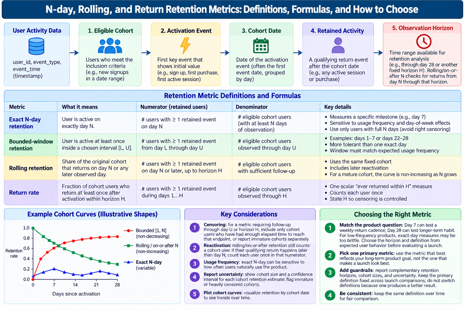
How would you define and choose among N-day, rolling, and return retention metrics? diagram
How to Explain It in an Interview

I would define the measurement population first. An eligible cohort is the set of users who meet the inclusion rule and complete the activation event. The activation event is the first qualifying event that represents initial value, such as a first active session. The cohort date is the date of that activation event, usually grouped by day. Retained activity is the later qualifying action that counts as a return. The observation horizon is the amount of follow-up time available for measuring retention.

For exact N-day retention, the numerator is the number of eligible cohort users with at least one retained event exactly on day N after the cohort date. The denominator is the number of eligible cohort users who have been observable for at least N days. This answers a narrow question such as, 'What fraction returned exactly on day 7?' It can be sensitive to day-of-week effects and to products that users naturally use less often than once per day.

For bounded-window retention over [L, U], the numerator is the number of cohort users with at least one retained event from day L through day U. The denominator contains eligible cohort users observed through day U. Examples are days 1 through 7 or days 22 through 28. A bounded window is more tolerant than one exact day because a user can return anywhere inside the chosen interval. If the lower bound is 1 and the upper bound grows with N, bounded [1, N] retention is cumulative and therefore cannot decrease as N grows for a fixed mature cohort.

For rolling retention at N, I would define the numerator as cohort users who have at least one retained event on day N or any later observed day, up to the available horizon H. The denominator is the eligible cohort with sufficient follow-up through that horizon. This definition includes later reactivation. If a user is inactive on day N but returns later, that user still counts. For a fixed mature cohort, rolling retention is non-increasing as N grows because the requirement becomes harder: the qualifying return must occur at an increasingly late time.

For return rate, I would use one explicit horizon H. The numerator is the number of eligible cohort users with at least one retained event during days 1 through H, and the denominator is the number of eligible cohort users observed through H. Each user counts once. This gives one scalar answer to, 'What fraction returned at least once within H?' With the same start and end points, this is mathematically the same event definition as bounded-window retention over [1, H]; the difference is usually how the result is presented and used.

Censoring matters because recent cohorts have not had enough time to reach the required endpoint. For an exact day-N metric, users need at least N days of follow-up. For a bounded interval ending at U, they need follow-up through U. For rolling retention evaluated through horizon H, they need follow-up through H. For a return rate ending at H, they also need follow-up through H. I would either restrict the denominator to mature users or clearly mark immature cohorts separately instead of treating missing future observation as non-retention.

Reactivation also changes the meaning of the metrics. Exact N-day retention ignores a user who misses day N but returns later. A bounded window counts the user only if the return happens inside that interval. Rolling retention counts a later return because it asks for activity on or after N. Return rate counts any qualifying return inside its fixed horizon H.

Seven-day and twenty-eight-day measures can answer different product questions. Day 7 may be useful when the product expects a weekly-return cadence or when the team wants an early signal of repeated value. Day 28 can test a longer-term habit. Neither horizon is automatically better. For a low-frequency product, exact-day retention can be brittle, so a bounded window or another definition may better match natural behavior. The important point is to select the definition from the expected usage pattern before looking at launch results.

I would report retention by cohort date rather than only one pooled number. For each cohort estimate, I would show cohort size and an uncertainty interval, such as a confidence interval for a retention proportion. I would flag immature or heavily censored cohorts. The curve shape itself is useful: exact N-day retention can move up or down across days, cumulative bounded [1, N] retention is non-decreasing, and rolling or on-or-after-N retention is non-increasing for a mature fixed cohort.

Finally, I would choose one primary retention metric based on the product question and expected user behavior, document the definition, and keep it fixed across launch comparisons. I would add guardrails such as complementary retention horizons, cohort sizes, uncertainty, and possibly another retention formulation. I would not switch from exact N-day to rolling or return rate simply because one definition gives a higher number. That would change the question being measured instead of evaluating the launch consistently.

Technical Approach
  1. Define the eligible user population and activation event.
  2. Assign each activated user a cohort date.
  3. Define the later activity that counts as retained activity.
  4. Choose the observation horizon required for mature follow-up.
  5. For exact N-day retention, count users active exactly on day N and divide by eligible users observable through N.
  6. For bounded-window retention, count users active at least once in [L, U] and divide by eligible users observable through U.
  7. For rolling retention, count users active on day N or any later observed day through H and divide by eligible users observable through H.
  8. For return rate, count users with at least one return during days 1 through H and divide by eligible users observable through H.
  9. Plot results by cohort date, show cohort size and uncertainty, and identify immature cohorts.
  10. Choose one primary definition from the product question and expected usage cadence before comparing launches, then use complementary retention measures as guardrails.
Practical Insights

The arithmetic is simple, but the measurement design is not. Exact N-day retention is easy to explain but can be noisy for irregular usage. Bounded windows are more forgiving, but the chosen interval changes the business meaning. Rolling retention captures later reactivation, but it answers a different question from exact-day retention. Longer horizons such as 28 days delay when a cohort becomes mature, so teams must wait longer before making a stable comparison. Reporting more cohorts and confidence intervals adds analysis work, but it reduces the risk of reacting to random variation or censored data.

Why Interviewers Ask This

This tests whether the candidate understands that retention is not one universal metric. The interviewer wants to see precise cohort and time definitions, correct numerators and denominators, proper handling of censoring and reactivation, awareness of usage frequency, uncertainty reporting, and disciplined metric selection that does not change simply because another definition makes a result look better.

Common interview mistakes

Common mistakes are mixing cohort definitions across analyses; failing to define activation or retained activity; putting recent users in a denominator before they have enough follow-up; calling a last-N-days active-user metric 'rolling retention' when the intended definition is return on or after day N; treating exact day 7 and return within seven days as the same metric; ignoring later reactivation; comparing seven-day and twenty-eight-day values as if they answer the same product question; reporting percentages without cohort sizes or uncertainty; pooling cohorts with different maturity; and changing the primary retention definition after seeing which one makes a launch look strongest.

Interview tip

Start with the cohort and time definitions before discussing formulas. Then contrast the four numerators and denominators, explain censoring and reactivation, and finish by saying that the primary metric must be chosen from product behavior before looking at launch results.
Interviewer may ask next
How would you handle a cohort that has only 10 days of follow-up when the primary metric is 28-day retention?

I would not treat those users as failures for a 28-day metric because their outcome is not observable yet. I would exclude that immature cohort from the mature 28-day denominator or display it separately as incomplete. For an exact day-28 metric, each user needs at least 28 days of follow-up. For a bounded interval ending at day 28 or a return rate through H = 28, the same maturity requirement applies. I could still report a mature seven-day metric for that cohort if enough time has elapsed, but I would clearly label it as a different question rather than substituting it for the primary 28-day result.

What would you do if exact day-7 retention falls after a launch but rolling retention improves?

I would not choose whichever number looks better. The two metrics measure different behavior. Exact day-7 retention asks whether users return exactly on day 7, while rolling retention asks whether they return on day 7 or later within the available horizon. I would first keep the preselected primary metric as the decision metric. Then I would inspect the cohort curves and complementary measures to understand the pattern. The result could mean users are returning later rather than at the weekly milestone. I would also check cohort size, uncertainty, usage-frequency changes, and censoring before deciding whether the difference is meaningful.

2. How would you compare shopping-surface ads with web-destination ads without making a causal claim from observational data?Model Evaluation And ValidationMediumMeta

Question Details

Use twenty-eight days of ad-detail and conversion data to define ad, advertiser, campaign, day, impression, click, conversion, spend, and value grains before joining. Compare shopping-destination and web-destination ads on exposure, click, conversion, value, and cost metrics after pre-aggregating to prevent many-to-many inflation. Explain advertiser, objective, placement, audience, budget, creative, and selection differences; choose weighting, stratification, or regression adjustments for a descriptive comparison; quantify uncertainty and sensitivity; inspect overlap and outliers; and state which causal conclusions remain unsupported without randomized assignment or a defensible natural experiment.

Short Interview Answer (30-60 seconds)

I would first aggregate every source to a common ad-by-day grain, then compare shopping-surface and web-destination ads on impressions, clicks, CTR, conversions, conversion rate, value, spend, ROAS, and CPA. I would adjust descriptively for observed group differences, report uncertainty, inspect overlap and outliers, run sensitivity checks, and avoid any causal claim without randomization or a defensible natural experiment.

Detailed Explanation

This is an observational comparison of two ad destinations over twenty-eight days. The goal is to describe how shopping-surface ads and web-destination ads differ, not to prove that destination type causes the difference. I would first define the natural grain of every source so joins cannot multiply rows. Then I would aggregate event data to a common ad-by-day grain, calculate exposure, click, conversion, value, and cost metrics, and compare the two groups. Because advertisers may select ad types differently, I would adjust for measured differences, quantify uncertainty, inspect overlap and outliers, test sensitivity, and keep the conclusion descriptive.

Useful Questions to Ask the Interviewer
  1. Is the twenty-eight-day window fixed, and should every ad be observed for the same calendar period?
  2. How are shopping-surface and web-destination ads identified in the ad-detail data?
  3. What attribution rule links a conversion and its value back to an ad and day?
  4. Are impression, click, and conversion tables event-level, or are any of them already aggregated?
  5. Which advertiser, objective, placement, audience, budget, creative, and selection variables are available before the outcome occurs?
  6. Should the comparison represent the observed ad population directly, or should advertisers receive equal influence?
  7. Are there minimum-volume rules or known invalid records that should be removed before computing rates?
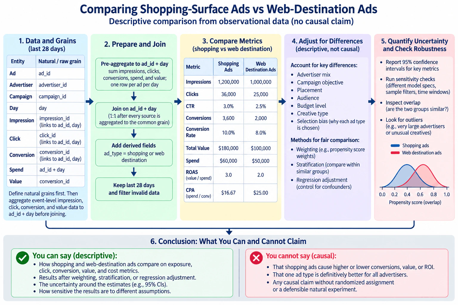
How would you compare shopping-surface ads with web-destination ads without making a causal claim from observational data? diagram
How to Explain It in an Interview
1. Define the grain before joining

A grain means what one row represents. I would write this down for every source before touching the joins.

For the approved design, the natural grains are:

  • Ad: one row per ad_id.
  • Advertiser: one row per advertiser_id.
  • Campaign: one row per campaign_id.
  • Day: one row per day.
  • Impression: one row per impression_id, linked to ad_id and day.
  • Click: one row per click_id, linked to ad_id and day.
  • Conversion: one row per conversion_id, linked to ad_id and day.
  • Spend: one row per ad_id + day.
  • Value: one value attached to each conversion, so its natural grain is conversion_id before aggregation.

The important failure case is joining raw impression, click, and conversion events directly. One ad can have many impressions, many clicks, and many conversions. Joining those many-to-many tables can multiply rows and inflate counts, spend, or value.

2. Pre-aggregate to a common grain

I would aggregate the event-level sources to ad_id + day. For each ad and day, I would sum impressions, clicks, conversions, spend, and conversion value. After every source used in the metric join has one row per ad per day, I would join on ad_id + day at that common grain.

I would also attach the ad attributes needed for comparison, including destination type, advertiser, campaign objective, placement, audience, budget, and creative information. I would keep the required twenty-eight-day window and filter invalid records using agreed data-quality rules rather than silently dropping inconvenient observations.

3. Build descriptive metrics

For each destination type, I would report both totals and rates because they answer different questions.

Exposure and volume:

  • Impressions.
  • Clicks.
  • Conversions.
  • Total value.
  • Spend.

Rates and efficiency:

  • CTR = clicks / impressions.
  • Conversion rate = conversions / clicks when clicks are the agreed denominator.
  • ROAS = value / spend.
  • CPA = spend / conversions.

The audited diagram uses an illustrative table where shopping ads have 1,200,000 impressions, 36,000 clicks, 3,600 conversions, $180,000 in value, and $60,000 in spend, while web-destination ads have 1,000,000 impressions, 25,000 clicks, 2,000 conversions, $100,000 in value, and $50,000 in spend. Those values illustrate the metric calculations and do not establish causation.

4. Explain why the raw comparison may be misleading

The two groups may differ before outcomes are measured. Shopping-surface ads and web-destination ads can have different advertiser mixes, campaign objectives, placements, audiences, budget levels, creative types, and selection processes. For example, advertisers may choose a destination type for campaigns that already have different goals or expected performance.

That means a raw difference can reflect destination type together with those observed selection differences. In simple terms, the groups may not be comparable before the outcome happens.

5. Adjust descriptively for measured differences

I would choose an adjustment method based on the available covariates and the amount of overlap between the groups.

Weighting: Estimate each observation's probability of being in its observed destination group from measured pre-outcome covariates, then use those probabilities to construct weights that make the observed covariate distributions more comparable. Propensity-score weighting is one possible approach.

Stratification: Put observations into comparable groups, such as similar advertiser, objective, placement, or propensity-score strata, and compare destination types within those groups before combining the descriptive results.

Regression adjustment: Model the outcome or metric as a function of destination type plus measured covariates such as advertiser, objective, placement, audience, budget, and creative. I would describe the destination term as an adjusted association, not a causal effect.

These methods can reduce imbalance in measured variables. They cannot guarantee that unmeasured differences have been removed.

6. Inspect overlap before trusting an adjusted comparison

Overlap asks whether similar observations exist in both destination groups. I would inspect covariate distributions or propensity-score distributions for shopping and web-destination ads.

If the groups barely overlap in an important region, an adjusted estimate may depend heavily on extrapolation or extreme weights. In that case I would narrow the comparison to the region with reasonable common support, report the limitation, and avoid claiming that one adjusted number represents all advertisers or ads.

7. Inspect outliers and influential observations

A very large advertiser, an unusual creative, an extreme budget, or an observation with a very large weight can dominate the comparison. I would inspect distributions, contribution to totals, and extreme weights or metric values.

I would not remove an outlier merely because it changes the result. I would determine whether it is invalid, genuinely part of the population, or a sign that the groups have weak overlap. Then I would report the main analysis and an appropriate sensitivity analysis.

8. Quantify uncertainty

I would report uncertainty for the main differences, such as 95% confidence intervals. The uncertainty method should match the structure of the data and the estimator. For example, if repeated ad-day observations from the same advertiser are correlated, the interval calculation should account for that dependence rather than treating every row as fully independent.

The point estimate tells me the observed size of the difference. The interval shows how precisely that difference is estimated. I would discuss both statistical uncertainty and practical size rather than treating a significance test as the whole conclusion.

9. Run sensitivity checks

I would repeat the comparison under reasonable alternative choices. Examples include different adjustment specifications, weighting approaches, strata, sample filters, and time windows. I would also check whether conclusions change when influential observations are handled differently under defensible rules.

If the direction and practical size of the result remain similar, the descriptive conclusion is more robust to those choices. If the result changes substantially, that instability is part of the answer and should be reported rather than hidden.

10. State the conclusion at the correct strength

I can say that, in these observational data, shopping-surface and web-destination ads differ on exposure, click, conversion, value, or cost metrics. I can report raw and adjusted descriptive comparisons, uncertainty, overlap, outliers, and sensitivity results.

I cannot say that shopping-surface ads cause higher or lower conversions, value, ROAS, or other outcomes. I also cannot say one destination type is definitively better for every advertiser. Weighting, stratification, and regression do not create randomized assignment. A causal conclusion would require randomized assignment or a defensible natural experiment with assumptions appropriate to that design.

Technical Approach
  1. Restrict the data to the required twenty-eight-day window and apply agreed validity rules.
  2. Document the natural grain and keys of ad, advertiser, campaign, day, impression, click, conversion, spend, and value data.
  3. Aggregate impression, click, conversion, value, and spend data to one row per ad_id + day.
  4. Join the aggregated sources on ad_id + day and attach destination type plus advertiser, objective, placement, audience, budget, and creative attributes.
  5. Compute impressions, clicks, CTR, conversions, conversion rate, value, spend, ROAS, and CPA for shopping-surface and web-destination ads.
  6. Examine raw differences in group composition.
  7. Choose weighting, stratification, or regression adjustment for observed differences and describe the result as an adjusted association.
  8. Inspect covariate or propensity-score overlap and influential observations.
  9. Report uncertainty, such as 95% confidence intervals, using a procedure appropriate for the dependence structure.
  10. Run sensitivity analyses with reasonable alternative specifications, filters, weighting choices, and time windows.
  11. Report descriptive findings and explicitly state that causal conclusions remain unsupported without randomized assignment or a defensible natural experiment.
Practical Insights

The data work is usually dominated by reading, aggregating, and joining the twenty-eight days of event data. Pre-aggregation adds a processing step, but it prevents much more serious many-to-many counting errors and reduces the size of later joins. Weighting is easy to summarize but can become unstable when some observations receive very large weights. Stratification is easy to explain, but many strata can become sparse. Regression can use many covariates, but its result depends on model specification. All three methods address only measured differences. Confidence intervals and sensitivity analyses add computation, but their main cost is analytical discipline: defining assumptions, checking overlap, investigating outliers, and explaining when the answer is unstable.

Why Interviewers Ask This

This question tests whether a candidate can make a disciplined comparison from observational data without turning association into causation. It checks data-grain reasoning, prevention of many-to-many join inflation, metric selection, adjustment for important group differences, overlap diagnostics, uncertainty, robustness, outlier analysis, and the judgment to state clearly what the available evidence does and does not support.

Common interview mistakes

Common mistakes are joining raw impression, click, and conversion events and creating many-to-many inflation; failing to define spend and value grains; comparing only totals when exposure differs; using inconsistent denominators for CTR or conversion rate; calling a regression coefficient or propensity-weighted difference a causal effect; adjusting for variables measured after the outcome or affected by destination choice; ignoring advertiser, objective, placement, audience, budget, creative, and selection differences; accepting extreme propensity weights without checking overlap; deleting outliers only because they are inconvenient; reporting point estimates without uncertainty; skipping sensitivity checks; and saying one destination is definitively better when the evidence is observational.

Interview tip

Start with grain and join safety, then move through metrics, group differences, adjustment, overlap, uncertainty, and sensitivity. Finish with one explicit sentence that the result is descriptive: weighting, stratification, or regression can adjust observed differences, but they do not justify causality without randomization or a defensible natural experiment.

Interviewer may ask next
What would you do if shopping-surface and web-destination ads have very poor propensity-score overlap?

I would not force a full-population adjusted comparison. Poor overlap means there are shopping ads for which comparable web-destination ads, or vice versa, are scarce or absent. I would identify the region of common support, inspect which advertisers or campaign types fall outside it, and consider restricting the descriptive comparison to observations with reasonable overlap. I would also inspect extreme weights because they can make the result depend on a small number of observations. I would report that the narrower estimate applies only to the supported population. I would not extrapolate the result to ads with no comparable observations, and I still would not make a causal claim.

What if the adjusted result changes substantially across weighting, stratification, regression, or different time windows?

I would treat that instability as an important result rather than choosing the method that gives the preferred answer. I would compare covariate balance, overlap, influential observations, and the assumptions behind each specification. I would report the range of reasonable estimates and explain which modeling or sample choices drive the change. A result that is highly sensitive to defensible choices is weaker descriptive evidence than a result that remains similar across them. The correct conclusion would emphasize uncertainty and sensitivity, and it would remain non-causal because the data are observational.

3. How would you estimate the short- and long-term revenue impact of a new ads-ranking model?Model Evaluation And ValidationHardMeta

Question Details

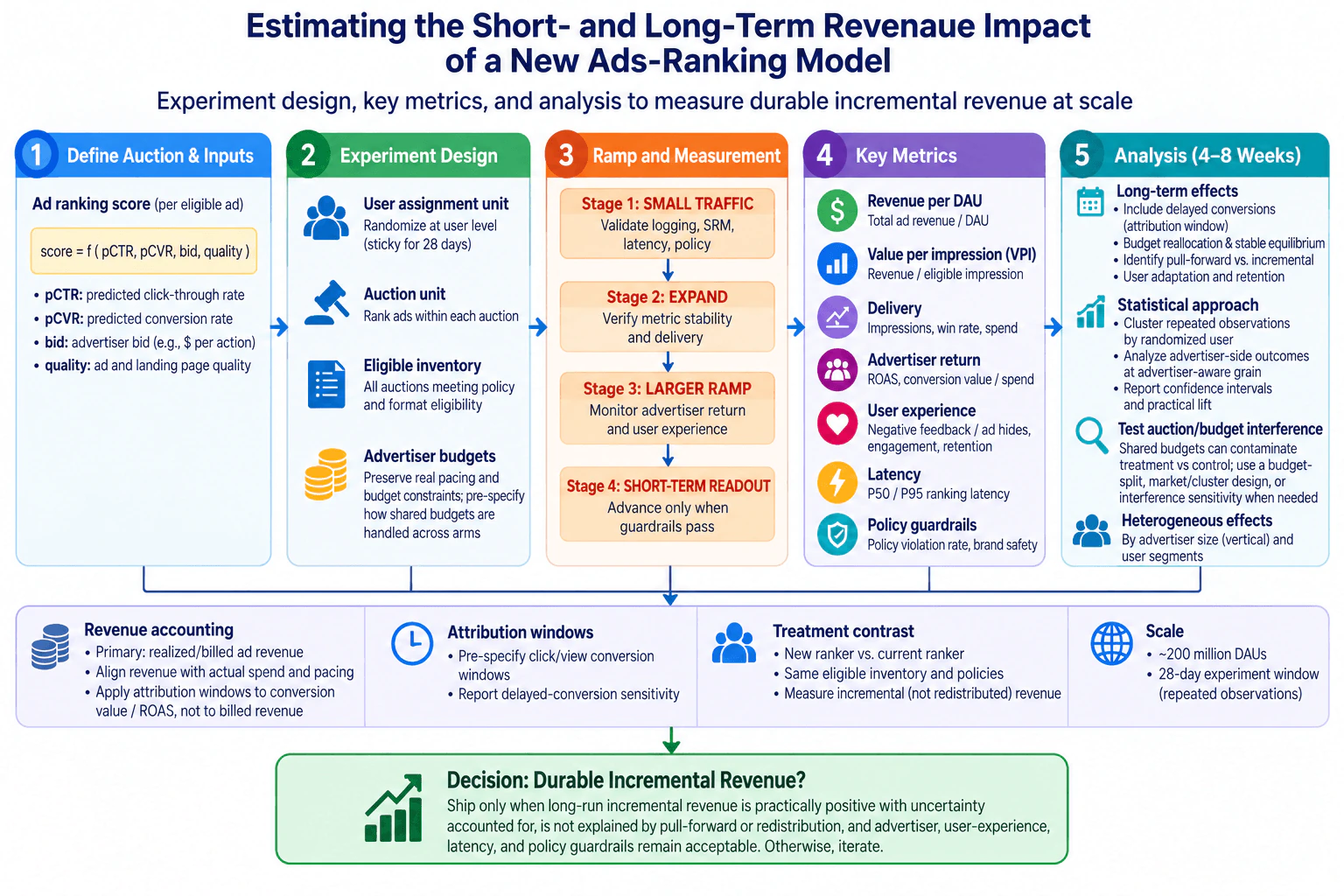
The ranker combines predicted click-through rate, predicted conversion rate, bid, and quality. Define the auction and user assignment units, eligible inventory, advertiser budgets, revenue accounting, attribution windows, and treatment contrast. Design a short ramp that measures revenue per daily active user, value per impression, delivery, advertiser return, latency, user experience, and policy guardrails, then a four- to eight-week analysis for delayed conversions, budget reallocation, pull-forward, user adaptation, and retention. Address roughly 200 million daily active users over a twenty-eight-day window, repeated observations, cluster-robust uncertainty, spillovers through auctions and budgets, ramp stages, sample-ratio and logging checks, heterogeneous advertisers and users, and a decision policy that separates durable incremental revenue from redistribution or short-term extraction.

Short Interview Answer (30-60 seconds)

I would randomize users between the current and new ranker, ramp gradually after SRM, logging, latency, policy, delivery, advertiser-return, and user checks pass, and estimate treatment-minus-control lift in revenue per DAU and value per impression. Then I would extend the analysis for four to eight weeks to capture delayed conversions, budget reallocation, pull-forward, retention, interference, and durable incremental revenue.

Detailed Explanation

The core task is to estimate causal revenue lift from the new ads ranker, not just whether its predictions look better offline. I would compare the new and current rankers on the same eligible auctions while keeping user assignment stable. The short ramp tells me whether revenue, delivery, advertiser return, latency, user experience, and policy guardrails remain healthy. The longer analysis asks whether the measured lift survives delayed conversions, budget movement, pull-forward, user adaptation, retention effects, and auction interference. The final decision should depend on durable incremental revenue with uncertainty, not a temporary redistribution of spend.

Useful Questions to Ask the Interviewer
  1. What exactly counts as platform revenue for this experiment: realized or billed ad revenue, and at what reporting grain?
  2. Which click-through and view-through conversion attribution windows should be pre-specified for advertiser-return analysis?
  3. Is user-level randomization operationally feasible for the full twenty-eight-day primary experiment window, and can assignment remain sticky?
  4. Which inventory, surfaces, markets, and policy-eligible ads are in scope for both treatment and control?
  5. How are advertiser budgets and pacing shared across treatment and control traffic today?
  6. Which user-experience and policy guardrails are considered launch blockers?
How would you estimate the short- and long-term revenue impact of a new ads-ranking model? diagram
How to Explain It in an Interview

I would start by defining the comparison precisely. The auction unit is each ad auction. Within an auction, eligible ads are ranked using the supplied score inputs: predicted click-through rate, predicted conversion rate, bid, and quality. The experimental assignment unit is the user, with sticky treatment assignment across the twenty-eight-day primary experiment window. Treatment uses the new ranker and control uses the current ranker. Both arms should use the same inventory eligibility and policy rules so that the treatment contrast is the ranking change rather than a population change.

Next I would define revenue and advertiser outcomes separately. The primary platform outcome is realized or billed ad revenue. For each day, revenue per DAU is that arm's ad revenue divided by that arm's daily active users. Across multiple days, I would preserve the same DAU-day grain rather than divide multi-day revenue by a single day's DAU. Value per eligible impression is a complementary measure because it separates monetization efficiency from changes in the number of impressions served. The causal short-term effect is the treatment-minus-control difference in these metrics, with a relative lift reported when useful. I would also track delivery, including impressions, win rate, and spend. Advertiser return is different from platform revenue, so I would evaluate measures such as ROAS or conversion value divided by spend using pre-specified click-through and view-through conversion windows. Those attribution windows apply to conversion value and advertiser return, not to billed platform revenue.

I would preserve real advertiser pacing and budget constraints because they are part of the auction environment. At the same time, shared advertiser budgets can create interference: treatment traffic can consume budget that otherwise would have been available to control traffic. That can contaminate a simple user-randomized estimate. I would therefore pre-specify how shared budgets are handled and test the sensitivity of the result to interference. Depending on feasibility, that can mean a budget-split design, a market or cluster-level design, or an explicit interference sensitivity analysis.

For the short ramp, I would use progressive exposure rather than assume fixed percentages or durations. The first stage is small traffic, where I validate logging, sample-ratio mismatch, latency, and policy behavior. If those checks pass, I expand and verify metric stability and delivery. At a larger ramp, I monitor advertiser return and user experience closely. I move to the short-term readout only when the guardrails pass. This staged approach limits risk while still producing evidence about the treatment effect.

The short-term scorecard should include revenue per DAU, value per eligible impression, delivery, advertiser return, ranking latency such as P50 and P95, user-experience measures such as negative feedback or ad hides and engagement, and policy guardrails. I would inspect sample-ratio mismatch, logging completeness, and metric consistency throughout. A revenue increase is not enough if it comes with unacceptable advertiser, user, latency, delivery, or policy damage.

The longer four-to-eight-week analysis answers whether the early revenue lift is durable. I would retain the original treatment assignment for the cohorts being compared and include delayed conversions using the pre-specified attribution windows. I would report sensitivity to those windows rather than treating the twenty-eight-day experiment duration as an attribution rule. I would look for budget reallocation and whether the marketplace is moving toward a different stable allocation of spend. I would test whether early revenue is merely pull-forward from later periods rather than genuinely incremental. I would also evaluate user adaptation, engagement, and retention because a ranker that extracts more revenue initially but harms longer-term usage may reduce durable value.

Because the same users contribute repeated observations across days, I would calculate uncertainty in a way that respects the randomized user assignment. For user-level outcomes, I would cluster repeated observations by randomized user and report confidence intervals together with practical lift, not only statistical significance. Advertiser-side outcomes should be analyzed at an advertiser-aware grain because advertiser budgets and pacing create dependence that is different from user-level repetition. I would also examine heterogeneous effects by advertiser size or vertical and by relevant user segments so that a positive average does not hide important losses in major cohorts.

Auction and budget spillovers need a separate check because ordinary user randomization assumes one user's treatment does not materially alter another arm's outcomes. Shared auctions, pacing, and budgets can violate that assumption. I would compare conclusions under an interference-aware design or sensitivity analysis when that risk is material. I would not call the observed treatment-control gap fully incremental if it can be explained by budget shifting between arms or advertisers.

Finally, I would separate three possibilities: true incremental revenue, redistribution, and short-term extraction. Redistribution means the ranker changes which advertisers or auctions receive spend without creating durable platform value. Pull-forward means revenue appears earlier but is offset later. Short-term extraction means monetization rises while advertiser return, user experience, retention, latency, or policy outcomes deteriorate. I would ship only when the long-run incremental revenue effect is practically positive after uncertainty is considered, the effect is not explained by pull-forward or redistribution, and advertiser, user-experience, latency, delivery, and policy guardrails remain acceptable. Otherwise, I would iterate rather than scale the ranker.

Technical Approach
  1. Define the auction unit as each ad auction and the treatment contrast as new ranker versus current ranker on the same eligible inventory and policy rules.
  2. Randomize at the user level and keep assignment sticky across the twenty-eight-day primary experiment window so repeated user observations remain in one arm.
  3. Preserve real advertiser pacing and budget constraints, and pre-specify how shared budgets across treatment and control will be handled.
  4. Define primary platform revenue as realized or billed ad revenue. Compute daily revenue per DAU and value per eligible impression, then estimate treatment-minus-control lift while preserving the correct daily or user-day denominator.
  5. Pre-specify click-through and view-through attribution windows for conversion value and ROAS, and plan sensitivity analysis for delayed conversions.
  6. Start with a small-traffic ramp and validate logging, sample-ratio mismatch, latency, and policy guardrails.
  7. Expand traffic only after checks pass, then verify metric stability and delivery.
  8. At larger exposure, monitor revenue per DAU, value per impression, delivery, advertiser return, user experience, latency, and policy outcomes.
  9. Continue into a four-to-eight-week analysis for delayed conversions, budget reallocation, pull-forward, user adaptation, engagement, and retention without re-randomizing the compared cohorts.
  10. Estimate uncertainty at the correct grain: cluster repeated user observations by randomized user and analyze advertiser-side outcomes at an advertiser-aware grain.
  11. Test auction and budget interference using an appropriate budget-split, market or cluster design, or interference sensitivity analysis when shared budgets can contaminate arms.
  12. Examine heterogeneous effects across advertiser and user segments.
  13. Ship only if long-run incremental revenue is practically positive with uncertainty accounted for, is not explained by pull-forward or redistribution, and all important guardrails remain acceptable.
Practical Insights

The main cost is not computational complexity but experimental and statistical complexity. With roughly 200 million daily active users, the data volume is large, but aggregation by user, day, advertiser, and auction makes the analysis manageable with distributed data systems. The harder problem is dependence: the same users appear repeatedly, and advertisers share budgets across auctions. That means naive row-level standard errors can be too optimistic. Longer experiments or follow-up also cost time because delayed conversions, budget reallocation, and retention cannot be measured immediately. More isolation, such as budget-split or cluster experiments, can reduce interference but may be operationally harder and may reduce statistical efficiency. The best design balances causal credibility, marketplace realism, risk, and time to decision.

Why Interviewers Ask This

This question tests whether a candidate can turn an ads-ranking change into a credible causal evaluation rather than simply comparing offline model metrics. The interviewer wants to see correct experiment units, revenue accounting, treatment contrast, staged ramping, business and user guardrails, repeated-observation uncertainty, delayed outcomes, heterogeneous effects, auction and budget interference, and a decision rule that separates durable incremental revenue from redistribution or short-term extraction.

Common interview mistakes

Common mistakes are randomizing impressions while ignoring repeated user exposure, changing eligible inventory between treatment and control, treating advertiser conversion attribution as the definition of platform revenue, using the twenty-eight-day experiment length as an attribution window, dividing multi-day revenue by a single day's DAU, declaring success from revenue alone, ignoring sample-ratio or logging problems, using naive independent-row standard errors for repeated users, clustering every outcome in the same way regardless of its grain, ignoring advertiser budget interference, inventing fixed ramp percentages without justification, stopping after a short-term readout, and calling redistributed or pulled-forward revenue durable incremental lift.

Interview tip

Present the answer as a causal measurement story: define the units and treatment first, explain what you measure during the safe ramp, then explain why the four-to-eight-week analysis is needed. Finish with the interference and uncertainty problem and a clear ship rule that distinguishes durable incremental revenue from redistribution or short-term extraction.

Interviewer may ask next
What would you do if user-level randomization shows a positive revenue lift but shared advertiser budgets may be contaminating treatment and control?

I would not treat the user-level estimate as automatically causal for the full marketplace effect. Shared budgets create interference because treatment traffic can change how much budget remains for control auctions. I would quantify that risk and, if material, use a design with stronger isolation such as advertiser budget splits or market or cluster randomization when feasible. If stronger isolation is not practical, I would run an interference sensitivity analysis and compare advertiser-level spend, delivery, and return patterns across arms. I would require the durable-revenue conclusion to remain credible under those checks before scaling.

What if the new ranker increases revenue per DAU during the first two weeks but the four-to-eight-week analysis shows weaker advertiser return and lower retention?

I would not ship based on the early revenue result. The longer analysis suggests the short-term gain may be extraction rather than durable incremental value. I would determine whether the effect comes from pull-forward, budget reallocation, worse advertiser efficiency, or user adaptation. I would also examine the affected advertiser and user cohorts and their uncertainty intervals. The decision rule requires long-run revenue to remain practically positive while advertiser return, user experience, retention, latency, delivery, and policy guardrails stay acceptable, so this result would lead me to iterate on the ranker.

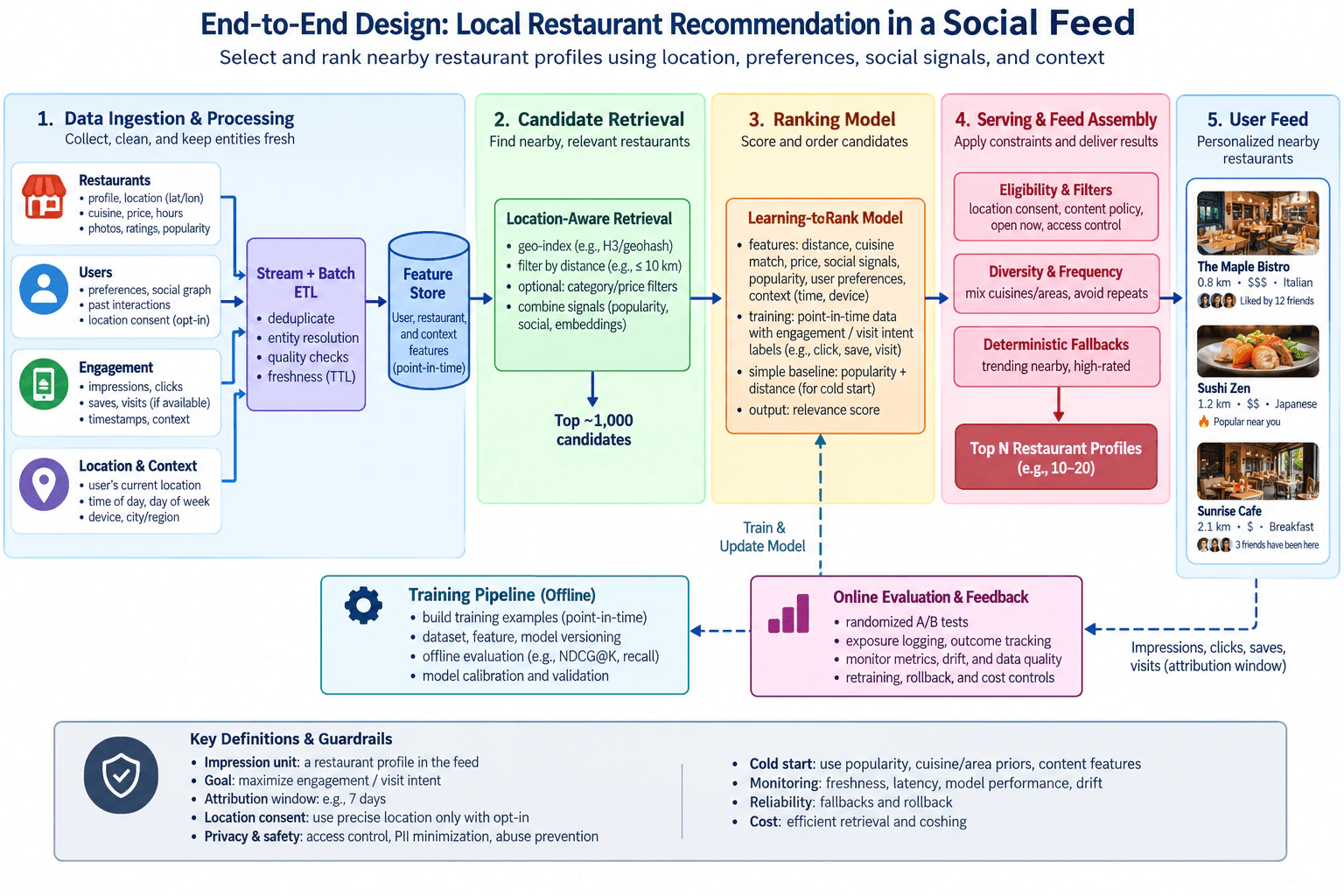
4. Design a system that recommends local restaurant profiles in a social feed.NEWMachine Learning System DesignEasyMeta

Question Details

Design an end-to-end system that selects and ranks nearby restaurant profiles for an eligible feed request. Define the user-profile impression unit, recommendation goal, engagement or visit-intent labels, attribution window, and location-consent boundary. Cover restaurant and user data ingestion, entity quality and freshness, distance, cuisine, price, social, popularity, and context features; candidate retrieval; a simple baseline and ranking model; point-in-time training examples; dataset, feature, and model versioning; low-latency serving with eligibility, diversity, frequency, and deterministic fallbacks; offline ranking and calibration tests; randomized online evaluation; exposure and outcome feedback; cold start, drift, retraining, monitoring, privacy-safe location use, access control, abuse prevention, reliability, rollback, and cost.

Short Interview Answer (30-60 seconds)

I would retrieve nearby eligible restaurants, rank them with point-in-time user, restaurant, social, and context features, then apply diversity and frequency rules before returning the feed. I would learn from logged impressions and later engagement or visit-intent outcomes, evaluate offline and through randomized A/B tests, and use consent-aware location, deterministic fallbacks, monitoring, retraining, and rollback.

Detailed Explanation

The system should decide which nearby restaurant profiles to show for an eligible social-feed request and in what order. The impression unit is one restaurant profile shown to one user in the feed. The goal is to maximize relevant engagement or visit intent while keeping results local, eligible, diverse, and fresh. Restaurant, user, engagement, location, and context data pass through quality-controlled processing. Location-aware retrieval narrows the catalog, a learning-to-rank model scores candidates, serving applies eligibility and feed constraints, and logged exposures and later outcomes create the feedback loop for evaluation and retraining.

Useful Questions to Ask the Interviewer
  1. What counts as success: clicks, saves, explicit visits, check-ins, or a weighted engagement or visit-intent objective?
  2. What location precision may be used, and should precise location require explicit opt-in at request time?
  3. How fresh must restaurant availability, hours, and profile information be before a restaurant can be recommended?
  4. Are there feed-level limits on repeated restaurants, cuisine concentration, area concentration, or frequency of exposure?
  5. What end-to-end latency and availability targets should the serving path meet?
  6. How should we treat users or restaurants with little or no interaction history?
Design a system that recommends local restaurant profiles in a social feed. diagram
How to Explain It in an Interview
1. Define the decision and impression unit

For each eligible feed request, the system selects and orders nearby restaurant profiles. One prediction corresponds to a user-restaurant candidate in the current request context. One impression is a restaurant profile actually shown to that user in the feed. The ranking model estimates relevance for engagement or visit intent, while the final feed also obeys eligibility, diversity, and frequency constraints.

The diagram uses an illustrative seven-day attribution window. A click, save, or qualifying visit signal that occurs after an impression can be joined back to that exposure when it falls inside this window. The exact attribution window is a product assumption to confirm with the interviewer, not a universal constant.

2. Enforce the location-consent boundary first

Precise current location is used only when the user has opted in. The request path checks consent before precise location participates in eligibility, retrieval, or ranking. Privacy-safe handling also means minimizing retained personally identifiable or precise location data, restricting access, and applying abuse-prevention controls. If consent is absent, the system must not silently use precise current location; it should use only an allowed coarser context or a deterministic non-personalized fallback when the product permits one.

3. Ingest and clean the source data

Restaurant inputs include profile information, latitude and longitude, cuisine, price, hours, photos, ratings, and popularity signals. User inputs include preferences, social-graph information, past interactions, and location-consent state. Engagement inputs include impressions, clicks, saves, and visits when a reliable visit signal exists. Request context includes current location when permitted, time of day, day of week, device, city, or region.

Stream and batch ETL perform deduplication, entity resolution, quality checks, and freshness handling. Duplicate restaurant entities should be resolved before training and serving so one physical restaurant is not represented as several recommendation entities. Freshness checks are especially important for changing attributes such as hours, availability, and profile status.

4. Build point-in-time features

The feature store holds user, restaurant, and context features. Important ranking features include geographic distance, cuisine match, price compatibility, social signals, popularity, user preferences, time, device, and freshness or quality signals.

Training examples must be point-in-time correct. For an impression at time t, every feature in the historical example must have been available at or before t. Later clicks, saves, or visits may become labels, but those later outcomes must never leak into the feature vector. This prevents point-in-time leakage and keeps training behavior aligned with information available during online serving.

The training pipeline versions the dataset, feature definitions, and model artifact together. This provides traceability between the data used for training, the feature logic, the evaluation result, and the model that is eventually served.

5. Retrieve a manageable candidate set

The online request first performs location-aware retrieval. A geographic index such as H3 or geohash can narrow the restaurant universe around the permitted user location. Distance, restaurant eligibility, and optional category or price filters reduce the set further. Popularity, social signals, and embeddings can contribute retrieval signals when available.

The diagram shows an example radius of at most 10 km and approximately 1,000 retrieved candidates. These are illustrative design values rather than fixed requirements. The purpose of retrieval is to maintain good recall while avoiding the cost of running the ranking model over the full restaurant catalog.

6. Rank the candidates

A simple baseline is popularity plus distance. It is inexpensive, interpretable, useful for comparison, and useful during cold start. The primary model is a learning-to-rank model that uses features such as distance, cuisine match, price, social signals, popularity, user preferences, and request context. It outputs a relevance score for each candidate.

Training should use exposure-based examples. Impressions establish which restaurant profiles actually had an opportunity to receive a later outcome. Labels may include clicks, saves, or reliable visit-intent signals within the agreed attribution window. A missing interaction should not automatically be interpreted as a strong dislike because many exposed items receive no action for reasons unrelated to relevance.

7. Validate offline before promotion

Offline evaluation should measure ranking quality with metrics such as NDCG@K and recall. Calibration should also be checked when the model score is interpreted as a probability-like engagement or visit-intent estimate. Point-in-time validation, data-quality checks, and comparison against the popularity-plus-distance baseline belong in the validation process. A model should not be promoted only because its training objective improved.

Dataset, feature, and model versions should be recorded with the evaluation result so a deployed model can be reproduced and a previous validated version can be restored during rollback.

8. Serve online and assemble the feed

For each eligible request, the serving path checks location consent and content or policy eligibility, retrieves nearby candidates, loads the required online features, scores candidates with the ranking model, and then performs feed assembly.

Eligibility checks include location consent, content policy, restaurant availability such as open-now when required, access controls, and abuse filters. After model scoring, the service applies diversity across cuisine or area and frequency controls to avoid showing the same restaurant repeatedly. It then returns the top restaurant profiles. The diagram shows 10 to 20 profiles as an illustrative output size rather than a fixed system requirement.

Model execution time is only one part of latency. End-to-end request latency also includes geographic retrieval, feature access, eligibility filtering, ranking, diversity and frequency processing, network overhead, and final feed assembly.

9. Handle cold start and failures safely

For a new user, the system can rely more on distance, popularity, cuisine or area priors, restaurant content features, and permitted request context until personalized history becomes available. A new restaurant can be scored using location, cuisine, price, hours, content, quality, and other non-interaction features.

If the learned ranking model is missing, times out, or cannot obtain required features, the service should degrade safely instead of failing the feed request. The deterministic fallback shown in the diagram can return eligible trending-nearby or high-rated restaurants, using stable signals such as distance and popularity for deterministic ordering. Stale or invalid restaurant entities should be filtered according to their freshness and quality status rather than blindly served.

Caching, efficient retrieval, overload protection, and safe fallback behavior help balance latency, reliability, and cost.

10. Evaluate online and close the feedback loop

A randomized A/B test compares the new ranking policy with the current production policy. Exposure logging records which restaurant profile was shown, to which user or eligible request, at what time, and under which model or configuration version. Later clicks, saves, and qualifying visit outcomes are joined back to those impressions using the attribution rule.

The online experiment should measure the chosen engagement or visit-intent objective together with guardrails such as feed quality, repeated exposure, latency, and reliability. Offline ranking quality alone is not enough to justify deployment because historical ranking metrics do not fully predict behavior under a new live recommendation policy.

11. Monitor the system and retrain carefully

Monitoring should separate different failure types. Service-health monitoring covers latency, errors, timeouts, and availability. Data-quality monitoring covers missing, duplicate, invalid, or stale entities and features. Drift monitoring checks changes in feature or score distributions, but drift by itself does not prove recommendation quality has declined. Model-quality monitoring uses delayed outcomes when they become available, while product monitoring follows engagement or visit-intent outcomes.

Retraining may be periodic or triggered by enough new labeled data or meaningful quality degradation. A new model must pass the same validation process before promotion. If the online experiment, reliability metrics, or safety signals deteriorate, the service should roll back to the previous validated model and configuration.

12. Main tradeoffs

A larger candidate set can improve recall but increases retrieval and ranking cost. Richer real-time features can improve relevance but add latency, availability dependencies, and training-serving-skew risk. Stronger diversity and frequency rules may lower the raw sum of model scores while improving the quality of the feed as a whole. Precise location can improve local relevance but creates a stronger privacy obligation, so consent and data minimization take priority. The final design therefore combines efficient location-aware retrieval, point-in-time-correct learning, online ranking, feed constraints, deterministic fallback behavior, and a closed exposure-to-outcome feedback loop.

Technical Approach
  1. Define one impression as one restaurant profile shown to one user, then define the engagement or visit-intent label and attribution window.
  2. Check location consent before using precise current location.
  3. Ingest restaurant, user, engagement, location, and context data with batch and streaming ETL.
  4. Deduplicate restaurant entities, resolve identities, validate fields, and enforce freshness rules.
  5. Build versioned user, restaurant, and context features with point-in-time correctness.
  6. Retrieve nearby candidates with a geographic index, distance and eligibility filters, plus optional category, price, popularity, social, or embedding signals.
  7. Keep a popularity-plus-distance baseline for comparison and cold start.
  8. Train a learning-to-rank model on exposure-based point-in-time examples using engagement or visit-intent outcomes.
  9. Evaluate ranking quality, recall, calibration, data quality, and baseline comparisons before promotion.
  10. At request time, retrieve candidates, load online features, score them, then apply eligibility, diversity, and frequency constraints.
  11. Return the top restaurant profiles, with deterministic trending-nearby or high-rated fallbacks if the learned model or required features are unavailable.
  12. Log exposures and outcomes, run randomized A/B tests, monitor service health, data quality, drift, model quality, and product outcomes, then retrain and roll back through the same validation process when needed.
Practical Complexity & Trade-offs

The expensive part is not only the ranking model. Geographic retrieval should first reduce a large restaurant catalog to a manageable candidate set, and the model then scores only those candidates. More candidates may improve recall but increase CPU, memory, feature reads, and latency. More real-time features can improve relevance but create additional dependencies and more chances for stale or missing data. Caching and efficient geographic indexing lower serving cost, but cached information can become stale. Diversity and frequency rules add post-processing work and may trade some raw ranking score for a better overall feed. Offline training also requires storage, feature computation, evaluation, retraining, and version-management cost.

Where it is used

This design is useful when a social or discovery feed must surface nearby restaurant profiles using both geographic relevance and user interest. It fits local-discovery experiences that combine location, social context, preferences, restaurant attributes, and request-time context while still enforcing eligibility, diversity, privacy, frequency control, and safe fallback behavior.

Why Interviewers Ask This

This question tests whether a candidate can turn a recommendation goal into a complete machine-learning system. The interviewer wants to see a correct impression and prediction unit, location-aware candidate retrieval, useful ranking features, leakage-safe training data, low-latency serving constraints, offline and online evaluation, privacy boundaries, and operational judgment. A strong answer also explains cold start, deterministic fallbacks, monitoring, feedback, retraining, rollback, reliability, abuse prevention, and cost.

Common interview mistakes

Common mistakes are treating the problem as only a ranking-model task; using precise location without checking opt-in consent; training with features that were not available at impression time; failing to log impressions before defining engagement labels; joining delayed outcomes to the wrong exposure or attribution window; failing to deduplicate restaurant entities; using stale hours or restaurant status; ranking the full catalog without a retrieval stage; ignoring a simple baseline; evaluating only a training metric; omitting calibration when score interpretation requires it; forgetting diversity or frequency controls; treating drift as proof that model quality declined; having no deterministic fallback for model or feature failures; and describing retraining without versioning, validation, monitoring, or rollback.

Interview tip

Start with the impression unit and location-consent boundary, then walk left to right through data quality, point-in-time features, candidate retrieval, ranking, feed constraints, evaluation, feedback, and safe degradation. Clearly separate model scoring from final feed assembly, and state that numbers such as 10 km, 1,000 candidates, 10 to 20 results, and seven days are illustrative assumptions from the design rather than universal requirements.

Interviewer may ask next
How would you handle a new user or a new restaurant with almost no interaction history?

For a new user, I would rely more on permitted request context, distance, popularity, cuisine or area priors, and restaurant content features. As impressions, clicks, saves, or reliable visit signals accumulate, personalization can receive more weight. For a new restaurant, I would use its location, cuisine, price, hours, content, and quality signals instead of interaction history. I would still enforce the same consent, eligibility, diversity, frequency, and abuse rules. If personalization is unavailable, the deterministic trending-nearby or high-rated fallback remains available.

What would you do if the learning-to-rank model improves offline NDCG but the online experiment reduces the engagement or visit-intent goal?

I would not promote the model based on the offline result. NDCG measures historical ranking quality, but it does not prove that the new policy improves behavior under live exposure. I would inspect experiment randomization, exposure and outcome joins, calibration, latency, repeated exposure, diversity, data quality, and segment-level outcomes. If the online degradation is real, I would keep or roll back to the previous validated model or fallback, correct the identified issue, retrain if appropriate, pass offline validation again, and run another randomized test before promotion.

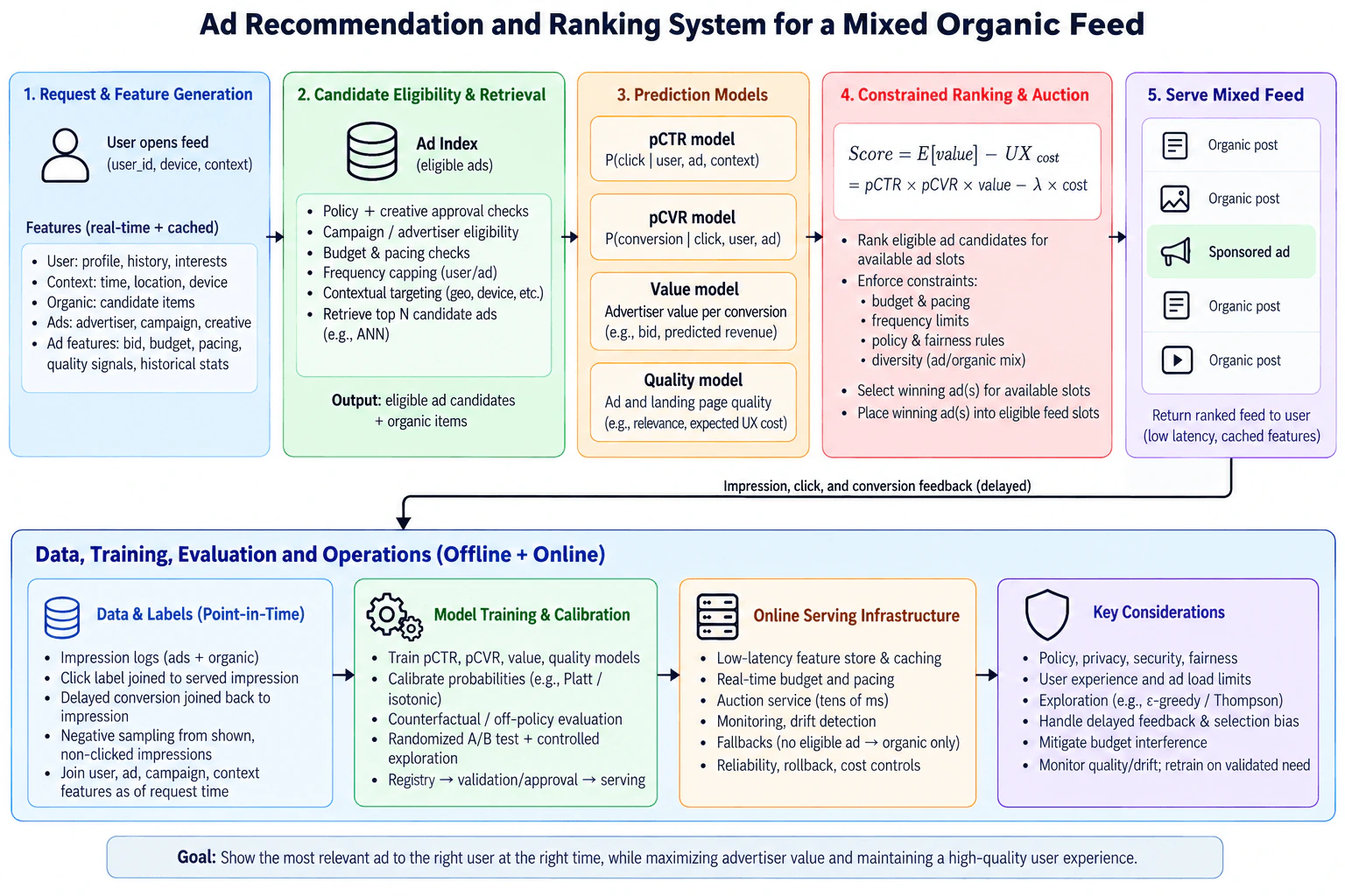
5. Design an ad recommendation and ranking system for a mixed organic feed.Machine Learning System DesignMediumMeta

Question Details

Design the end-to-end path that chooses an eligible ad and places it among organic feed items. Define the auction or impression unit, click and delayed conversion labels, advertiser value, user-experience costs, and policy constraints. Cover ad, advertiser, campaign, user, context, creative, bid, budget, pacing, quality, and historical features; candidate eligibility and retrieval; calibrated pCTR, pCVR, value, and quality models; a constrained ranking objective; point-in-time datasets, negative sampling, exploration, registry, and approval; low-latency online features, auction execution, caching, frequency limits and fallbacks; offline calibration and counterfactual checks; randomized online evaluation; delayed feedback, selection bias, budget interference, drift, retraining, monitoring, privacy, security, fairness, reliability, rollback, and cost.

Short Interview Answer (30-60 seconds)

I would retrieve only policy-approved, budget- and pacing-eligible ads, score them with calibrated pCTR, pCVR, advertiser value, and quality or UX cost, rank them under auction and frequency constraints, and place the winner into an eligible feed slot. Then I would learn from impression, click, and delayed conversion feedback using point-in-time training data.

Detailed Explanation

The system makes one practical decision: for an eligible advertising opportunity inside an organic feed, choose an eligible ad and place it in an allowed feed slot. I would build the path as request features → eligibility and retrieval → calibrated prediction models → constrained ranking and auction → mixed-feed serving. Training data is joined at the served-impression grain so clicks and delayed conversions return to the prediction that caused the impression. The design must balance advertiser value with user experience while respecting policy, budget, pacing, frequency, privacy, security, fairness, latency, reliability, and cost.

Useful Questions to Ask the Interviewer
  1. Is the feed layout already producing eligible ad slots, or should this system also decide whether an ad slot is available?
  2. What advertiser objective should value represent: clicks, conversions, or another campaign objective?
  3. How should delayed conversions be attributed back to served impressions?
  4. Which policy, frequency, pacing, and user-experience constraints are hard constraints rather than ranking penalties?
  5. Are pCTR and pCVR required to be calibrated probabilities because they feed directly into the auction value calculation?
  6. How fresh must budget, pacing, frequency, and contextual features be at serving time?
  7. What should happen when features, models, budget state, or eligible ads are unavailable?
  8. Which advertiser, user-experience, fairness, reliability, and cost outcomes should the randomized online experiment use as decision criteria?
Design an ad recommendation and ranking system for a mixed organic feed. diagram
How to Explain It in an Interview
1. Define the decision and the prediction grain

The online decision happens when a user opens or refreshes the feed and the system has an eligible advertising opportunity among organic items. The prediction grain is one candidate ad for one user and request context. The served impression is the key outcome grain because a later click or conversion must be joined back to the exact ad exposure and prediction that produced it.

The primary functional requirement is to return a mixed feed in which any sponsored item was first found eligible, then scored and selected under auction and product constraints. Organic posts do not participate as bidders in the ad auction. The auction ranks eligible ad candidates for available ad slots, and the winning ad is placed into an eligible position among organic content.

2. Build the request and feature contract

At request time, build a feature-rich context using the same logical feature definitions used during training. User features can include profile, historical behavior, and interests. Context features include device, location, time, and feed context. Ad-side information includes the ad, advertiser, campaign, creative, bid, budget, pacing, quality signals, and historical statistics. Organic candidates are available to the feed assembler because the final product is a mixed feed, although the ad auction itself ranks only ad candidates for eligible ad slots.

Feature availability time matters. A historical training row may use only information that would have been available when that request occurred. This point-in-time rule prevents future information from leaking into training. Online feature definitions should match offline definitions to reduce training-serving skew. Budget, pacing, and frequency state need especially fresh online values because they change as impressions are served.

3. Retrieve only eligible ad candidates

The first serving-stage reduction is eligibility, not ML ranking. Start from the ad index and apply policy and creative approval checks, campaign and advertiser eligibility, budget and pacing checks, frequency caps, contextual targeting, and any other required constraints. Then retrieve a manageable top-N candidate set, using user, context, and ad representations when approximate nearest-neighbor retrieval is appropriate.

This ordering is important. A model must not make an otherwise prohibited ad acceptable merely because it predicts high value. Hard policy and eligibility requirements remain constraints around the prediction system.

If no ad survives eligibility, the safe fallback is to return the organic feed without an ad rather than violating a constraint.

4. Predict click, conversion, advertiser value, and quality

For each eligible candidate, produce calibrated predictions that support the auction decision.

pCTR estimates P(click | user, ad, context).

pCVR estimates P(conversion | click, user, ad), consistent with the diagram. Because conversion feedback can arrive much later than the impression or click, the label pipeline must account for that delay rather than immediately treating unresolved outcomes as permanent negatives.

Advertiser value represents the economic value associated with the campaign objective, using the applicable bid or value information. A quality model represents ad and landing-page quality, relevance, and expected user-experience cost.

Calibration matters because predicted probabilities are used in an economic score. A model can rank candidates well but still produce poorly calibrated probabilities, which can distort expected value. I would therefore evaluate calibration offline and apply a suitable calibration method when needed rather than relying only on ranking discrimination.

5. Use a constrained ranking objective

A useful conceptual objective is:

Score = expected advertiser value - λ × expected UX cost.

For the conversion-value formulation shown in the diagram, expected advertiser value can be represented as pCTR × pCVR × advertiser value. The coefficient λ controls how strongly the system penalizes expected user-experience cost.

The score is not the whole decision. The auction still enforces hard constraints such as budget, pacing, frequency limits, policy and fairness rules, and allowed ad placement. The system ranks eligible ad candidates for the available ad slots, chooses the winner, and places the winning ad into an eligible feed position.

This separation between objective and constraints is important. Mandatory requirements should not be reduced to weak soft penalties when violating them is not allowed.

6. Build point-in-time training examples

The offline dataset starts from served impression logs. Each training row represents what the system actually knew when an ad was served. User, ad, advertiser, campaign, creative, context, and historical features are joined as of request time.

The click label is joined to the served impression. A delayed conversion is later joined back to the corresponding impression through the feedback contract. For click modeling, shown but non-clicked impressions provide observed negative examples. Unshown ads should not automatically be labeled as ordinary negative clicks because their outcomes were never observed.

Deduplicate repeated events and maintain stable request, impression, candidate, prediction, and outcome identifiers so feedback attaches to the correct entity and time. Version data definitions, features, model configuration, code, model artifacts, and evaluation results so an approved model can be reproduced and audited.

7. Handle selection bias and exploration

Historical logs come from previous retrieval and ranking policies, so they are selected data rather than a random sample of every possible ad-user pair. We mainly observe outcomes for candidates the old system chose to expose. That creates selection bias.

Use controlled exploration to collect information outside the deterministic choices of the current ranker. Counterfactual or off-policy evaluation can provide additional offline evidence when its assumptions are satisfied. If an estimator requires action propensities, log them correctly at decision time. Counterfactual checks do not replace randomized online testing because auction competition, user behavior, and budget interactions can violate simple offline assumptions.

8. Train, calibrate, validate, and approve models

The offline pipeline trains the pCTR, pCVR, advertiser-value, and quality components from point-in-time datasets. Evaluate predictive quality and probability calibration separately. Also inspect important slices for users, advertisers, campaigns, creatives, contexts, and applicable fairness requirements rather than approving a model from one aggregate metric.

Before serving, a model artifact goes through validation and approval and is stored in a model registry with its lineage. The registry records a versioned artifact; registry entry alone is not a deployment decision. The lifecycle is registry → validation and approval → serving.

A new model should not launch only because a training or offline metric improved. It must also satisfy relevant data-quality, calibration, policy, reliability, fairness, and online-evaluation gates.

9. Serve predictions with low latency

Online serving uses low-latency online features plus cached information where freshness allows it. The request goes through eligibility, candidate retrieval, prediction, constrained ranking, auction execution, and feed assembly. End-to-end request latency includes all of those stages, so it is different from model inference latency alone.

Real-time state such as remaining budget, pacing, and frequency counts must be incorporated close enough to the auction decision that the system does not repeatedly serve ads using stale eligibility state. Caching should distinguish relatively stable features from state whose freshness directly affects constraints.

The serving path must handle timeouts, stale or missing features, unavailable models, overload, and empty candidate sets. Safe degradation can use valid cached or default-safe features, a previously approved model when appropriate, or an organic-only response when no valid ad decision can be made. Fallback behavior must never bypass policy, budget, pacing, or frequency constraints merely to fill an ad slot.

10. Update state and collect feedback

After serving, log the request, the information needed to reconstruct the eligible decision set, feature or feature-version references, predictions, the winning decision, auction information needed for evaluation, and the served impression. The serving system updates relevant budget, pacing, and frequency state.

Clicks can arrive soon after the impression, while conversions may arrive much later. Both must be joined to the original served impression and prediction. This creates the delayed-feedback loop back into the point-in-time training dataset.

The delay is a modeling issue as well as a data-engineering issue. Training on examples whose conversion window has not matured can incorrectly create negative labels. The label-building process therefore needs a defined maturity or censoring policy consistent with the conversion definition rather than pretending every unresolved conversion is negative.

11. Evaluate offline and online

Offline, evaluate predictive quality, probability calibration, data quality, relevant slices, and decision quality where appropriate. Run counterfactual or off-policy checks carefully because historical exposure was selected by earlier policies.

Online, use a randomized experiment with controlled exploration where appropriate. Evaluate advertiser outcomes together with user-experience guardrails, fairness and policy measures, service reliability, and cost. The exact success metric should follow the product objective agreed with the interviewer rather than being invented.

Budget interference deserves special attention. Campaigns have finite budgets, so treatment and control can compete for the same advertiser resources. One arm can change spend or eligibility available to the other, breaking the simple assumption that experimental units are independent. The experiment design and analysis should account for this interference instead of treating a naive user-level A/B test as automatically unbiased.

12. Monitor the right layers separately

Monitor several classes of signals rather than combining everything into one health score.

Service health: end-to-end latency, errors, timeouts, overload, cache or dependency failures, and availability.

Data quality: missing, stale, duplicated, malformed, or unexpectedly distributed features and events.

Model behavior: prediction distributions, calibration, slice quality, and validated model-quality measures.

Drift: changes in features, labels, candidates, traffic, or predictions. Drift is a warning signal, not proof that model quality became worse.

Business and UX outcomes: advertiser value, spend, budget and pacing behavior, ad load, user-experience outcomes, and other agreed product measures.

Fairness and policy: relevant delivery or outcome slices and violations of approved constraints.

Cost: feature computation, retrieval, model inference, storage, logging, experimentation, and operational overhead.

13. Retraining and rollback

Retraining should happen because validated evidence says the production model or data needs updating, not merely because a fixed calendar interval elapsed. Useful triggers can include enough matured new labels, demonstrated quality degradation, sustained distribution change accompanied by quality evidence, or meaningful feature or product changes.

The new artifact still passes validation and approval before serving. If an online launch causes model-quality, UX, fairness, reliability, or business regressions, the serving layer should be able to route traffic back to the previous approved model and compatible configuration. Data, feature, configuration, and model versions must be recorded so rollback restores a coherent serving state rather than only swapping a model file.

14. Privacy, security, fairness, reliability, and cost

Use only data permitted for the advertising purpose and minimize unnecessary personal data. Apply access controls and protect data, feature, model, and serving interfaces from unauthorized access or tampering. Policy and creative approval are enforced before auction ranking rather than being left for the model to infer implicitly.

Fairness must be evaluated in the context of the actual ad-delivery decision and applicable constraints. A strong aggregate ranking metric does not establish fair behavior across relevant delivery or outcome slices.

For reliability, design the path so optional prediction improvements can degrade safely while mandatory eligibility constraints remain intact. For cost, reserve expensive computation for candidates that survive early filtering, cache reusable features when freshness allows it, and evaluate whether extra feature or model complexity creates enough decision value to justify its serving and maintenance cost.

Final decision

The complete loop is: build request features → enforce eligibility and retrieve candidates → predict calibrated pCTR, pCVR, advertiser value, and quality → rank eligible ads with a constrained auction objective → place the winner into an eligible feed slot → update serving state → record the impression → join click and delayed conversion feedback → rebuild point-in-time training data → validate and approve improved models → test them through randomized online evaluation. The system succeeds only when advertiser value, user experience, policy compliance, fairness, reliability, and cost remain acceptable together.

Technical Approach
  1. Define the advertising opportunity and use the served impression as the outcome and feedback grain.
  2. Build request-time user, context, organic-feed, ad, advertiser, campaign, creative, bid, budget, pacing, quality, and historical features with point-in-time semantics.
  3. Apply policy and creative approval, campaign and advertiser eligibility, budget and pacing checks, frequency caps, and contextual targeting before ranking.
  4. Retrieve a manageable set of eligible ad candidates.
  5. Produce calibrated pCTR and pCVR predictions plus advertiser-value and quality or UX-cost estimates.
  6. Rank eligible ads with an expected-value objective such as expected advertiser value minus a weighted UX cost while keeping hard policy, budget, pacing, frequency, fairness, and placement requirements as constraints.
  7. Run the auction for the available ad slot, choose the winning ad, and place it into the mixed organic feed.
  8. Serve through low-latency online features and caching while keeping fast-changing budget, pacing, and frequency state sufficiently fresh.
  9. Log requests, predictions, decisions, impressions, clicks, and delayed conversions at consistent identifiers and times.
  10. Build point-in-time training data from served impressions; use shown non-clicked impressions as click negatives and join delayed conversions back to the correct impression.
  11. Use controlled exploration and careful counterfactual evaluation to reduce blind spots created by historical selection bias.
  12. Train and calibrate models, validate data and model quality, register versioned artifacts, obtain approval, and only then make them eligible for serving.
  13. Compare approved changes with randomized online experiments, accounting for budget interference and checking advertiser, UX, fairness, reliability, and cost outcomes.
  14. Monitor service health, data quality, drift, model quality, calibration, policy, fairness, business outcomes, and cost separately.
  15. Retrain on validated need and retain a coherent rollback path to a previously approved model and compatible configuration.
  16. Fall back safely to an organic-only response when no valid ad can be selected.
Practical Complexity & Trade-offs

The main online cost comes from how many ads survive retrieval and how expensive their features and prediction models are. Early eligibility filtering reduces unnecessary scoring work. Approximate retrieval and cached features can reduce latency, but stale budget, pacing, or frequency state can produce invalid decisions, so not every feature should be cached for the same duration. More complex pCTR, pCVR, value, and quality models may improve ranking but increase inference cost, operational complexity, and failure risk. Offline pipelines also cost more because delayed conversions, point-in-time joins, exploration logs, calibration, counterfactual evaluation, and versioned artifacts must be maintained correctly. Experimentation is statistically difficult because campaign budgets create interference between decisions. Retraining too often wastes compute and can react to noise; retraining too slowly can leave the system stale. Reliability therefore requires safe degradation, monitoring, versioned configuration, and rollback rather than relying only on model accuracy.

Where it is used

This design is useful whenever sponsored content must be selected and inserted into a feed that primarily contains organic content. It applies when advertisers provide campaigns, creatives, bids, budgets, pacing, and targeting constraints while the platform must also protect user experience, policy requirements, frequency limits, fairness, privacy, security, and reliability. The same structure is useful when click and conversion feedback arrive at different times, when online decisions depend on rapidly changing budget or pacing state, and when ranking changes must be evaluated through controlled experiments rather than only offline model metrics.

Why Interviewers Ask This

This question tests whether I can connect recommendation modeling with auction economics and production ML. I need to define the prediction and impression grain, build leakage-safe labels and features, retrieve only eligible ads, calibrate pCTR and pCVR, combine advertiser value with user-experience cost, and enforce budget, pacing, policy, frequency, and placement constraints. It also tests whether I understand delayed feedback, selection bias, randomized evaluation, low-latency serving, reliability, privacy, security, fairness, monitoring, retraining, rollback, and the difference between a good offline model and a safe production system.

Common interview mistakes

Common mistakes are ranking every ad before checking eligibility; treating organic posts as bidders in the ad auction; using unshown ads as ordinary negative click labels; leaking future information into historical features; failing to join clicks and delayed conversions to the exact served impression; training on immature conversion labels as if they were final negatives; optimizing pCTR alone and ignoring conversion value, quality, and UX cost; using uncalibrated probabilities directly in an economic score without checking calibration; converting mandatory policy or budget rules into weak score penalties; ignoring budget, pacing, and frequency freshness; assuming model inference time equals total serving latency; launching a model because one offline metric improved; using counterfactual evaluation without considering selection and propensity assumptions; treating drift by itself as proof of quality loss; running a naive randomized test without considering budget interference; allowing fallback behavior to bypass policy or frequency rules; retraining on a fixed cadence without validated need; and rolling back only the model while leaving incompatible features or configuration active.

Interview tip

Draw the serving path first: request → eligibility and retrieval → prediction → constrained auction → mixed feed. Then add the feedback loop underneath. Define the served impression as the label grain, explain why pCTR and pCVR need calibration, separate hard constraints from the ranking objective, and finish with delayed feedback, randomized evaluation, safe fallback, monitoring, retraining, and rollback. This keeps a broad system-design answer structured instead of turning it into a list of unrelated components.

Interviewer may ask next
How would you train the conversion model when conversions can arrive long after the ad impression?

I would keep the served impression as the anchor and join any later conversion back to that impression through stable identifiers and event time. I would not immediately label every impression with no current conversion as a final negative because its conversion window may still be open. The label pipeline should use the agreed conversion-attribution and maturity rules so examples enter training with the correct known outcome or an explicitly handled censored state. The training features must still be point-in-time features from the original request, not information learned after the impression. I would monitor label delay and completeness because a change in reporting lag can look like model degradation even when user behavior has not changed.

What changes if campaign budgets are small enough that the randomized experiment's treatment and control groups compete for the same budget?

Then ordinary user-level independence becomes questionable. A treatment that wins impressions differently can consume a campaign's budget earlier, changing which ads remain eligible for control users and vice versa. That is budget interference. I would design the experiment and analysis so this shared-resource effect is explicitly considered rather than reading a naive user-level A/B difference as an unbiased treatment effect. The exact experimental unit or isolation strategy depends on the serving and campaign constraints, but both arms should use the same logging and policy contracts. I would also inspect spend, pacing, eligibility, advertiser value, UX outcomes, fairness, and reliability together so an apparent ranking gain is not actually caused by one arm taking budget from the other.

6. Design a safe process for replacing a legacy ads model with a new model.NEWMachine Learning System DesignHardMeta

Question Details

A legacy ads model M0 is a production dependency and candidate M1 changes ranking scores. Define immutable model and feature contracts, advertiser and user outcomes, attribution windows, budget interactions, and rollback authority. Reconstruct point-in-time training data, compare calibration and segment behavior over a twenty-eight-day offline window, and use logged propensities for inverse-propensity or doubly robust off-policy estimates with clipping and overlap diagnostics. Design shadow scoring, parity checks, user-bucket or geographic experiments, advertiser, revenue, delivery, latency, policy and user-experience guardrails, and a 1%, 10%, 25%, 50%, 100% ramp with automated stop conditions. Cover registry promotion, reproducibility, production serving and score compatibility, delayed feedback, drift, retraining, monitoring, incident recovery, privacy, security, reliability, and cost.

Short Interview Answer (30-60 seconds)

I would replace M0 with M1 through reversible gates. First freeze contracts and rebuild 28 days of point-in-time data. Then validate calibration, segments, and clipped IPS or doubly robust estimates, shadow M1 in production, experiment on isolated traffic, and ramp 1%, 10%, 25%, 50%, 100% only while guardrails pass. M0 stays ready for rollback.

Detailed Explanation

The safe design is a sequence of reversible gates from M0 to M1. M1 changes ranking scores, so I would first make the model, feature, and score interfaces immutable and define advertiser outcomes, user outcomes, attribution windows, budget interactions, and rollback authority. I would reconstruct the previous 28 days using point-in-time features so training or evaluation never sees future information. Offline evidence combines calibration and segment behavior with logged-propensity off-policy estimates. M1 then runs in shadow mode, followed by isolated experiments and the 1%, 10%, 25%, 50%, 100% ramp. Any guardrail breach stops the rollout or restores M0.

Useful Questions to Ask the Interviewer
  1. Which advertiser, revenue, delivery, policy, latency, and user-experience outcomes are release-blocking guardrails?
  2. What attribution windows define when delayed advertiser and user outcomes are considered complete enough for evaluation?
  3. Which logged propensities are available, and were they recorded at the same decision grain needed for IPS or doubly robust evaluation?
  4. Does M1 preserve the score interface expected by downstream ranking, pacing, and serving components, or is a compatibility layer required?
  5. Who has rollback authority, and which guardrail violations must trigger an automatic rollback instead of a manual review?
Design a safe process for replacing a legacy ads model with a new model. diagram
How to Explain It in an Interview
1. Freeze the contracts before comparing models

Treat M0 as a production dependency, not just a model file. Version the model artifact, feature definitions, feature schemas, joins, configuration, and score contract. The score contract defines the output format, range, semantics, and version expected by downstream systems. Also define advertiser and user outcomes, attribution rules, budget pacing and bidding constraints, and rollback authority before M1 receives production traffic.

This prevents a misleading comparison where M1 appears better because its inputs, score interpretation, or outcome definitions silently changed. Preserve lineage for the versioned data reconstruction logic, code, feature definitions, configuration, model artifacts, and evaluation results so the exact candidate can be reproduced.

2. Reconstruct a point-in-time 28-day offline window

Build the evaluation data exactly as it would have been known at each historical decision time. A feature value is eligible only if it was available at that time. This prevents future leakage and point-in-time errors. Requests, feature values, predictions, and eventual outcomes must stay joined at the correct entity and time grain.

Compare M0 and M1 over the required 28-day window. Check calibration, meaning whether predicted scores remain aligned with observed outcomes, and inspect behavior by relevant user, advertiser, and geographic segments. Segment checks matter because an aggregate improvement can hide a serious regression for one population.

3. Use logged propensities for off-policy evidence

Historical ads were selected by M0 or another logging policy, so the observed outcomes are biased toward actions that policy chose. Logged propensities record the historical probability of the chosen action. Use inverse-propensity scoring or a doubly robust estimator to estimate how M1 might behave without broadly serving it.

Clip importance weights so a small number of very unlikely logged actions cannot dominate the estimate. Then inspect overlap diagnostics. Poor overlap means M1 favors decisions that historical traffic rarely explored. In those regions, the off-policy estimate is weak evidence, so report the uncertainty instead of trusting one aggregate estimate.

Offline evaluation is a gate, not proof that M1 is safe. It cannot fully reproduce production budget interactions, auction effects, delayed user behavior, service failures, or strategic advertiser responses.

4. Shadow M1 before exposing users

In production shadow mode, M0 continues to serve the real ranking while M1 receives the same eligible inputs and produces scores that are logged but not served. This validates the production scoring path without changing user or advertiser outcomes.

Compare score distributions, feature parity, missing-feature rates, feature coverage, end-to-end latency, error rates, and policy or safety behavior. Confirm that online features match the versioned offline definitions and that M1's score format and semantics are compatible with downstream ranking and serving components. Shadow mode can expose training-serving skew and operational defects, but it cannot measure causal business impact because users still receive M0's decisions.

5. Run a controlled online experiment

After offline and shadow gates pass, assign traffic using stable user buckets or a geographic experiment design appropriate to the system. Keep treatment assignment isolated so the same user is not repeatedly switched between M0 and M1 in a way that contaminates measurement.

Measure advertiser, revenue, delivery, latency, policy, and user-experience outcomes over the predefined attribution windows. Relevant outcomes include advertiser conversions, CPA, ROAS, budget pacing and delivery; revenue and impression delivery; user relevance and experience; end-to-end latency and errors; and policy or safety violations.

Ads systems can have interference through auctions and budgets. A ranking change can alter which advertisers spend, when budgets exhaust, and which opportunities remain for later requests. That is why pacing and budget delivery are explicit guardrails rather than assuming every observation is independent.

6. Ramp gradually with automated stop conditions

If the controlled experiment passes, expose M1 using the required sequence: 1%, 10%, 25%, 50%, then 100%. Each step is a gate rather than a timer. Advance only after predefined guardrails remain acceptable for the required observation period.

Automated stop conditions should cover advertiser outcomes, revenue, delivery, latency, policy, and user experience. Service-health and data-quality failures should also block promotion because a statistically promising model is unsafe when the serving path is unhealthy.

Do not invent universal numeric thresholds. Agree on thresholds and decision rules before launch using product risk and operational requirements. If a release-blocking condition fires, stop further exposure and invoke the predefined rollback path. Automated rollback can restore M0 for configured breaches, while the authorized on-call team retains manual rollback authority.

7. Promote only the tested artifact

Promote only the exact M1 artifact that passed offline, shadow, and experiment gates. The registry entry should reference the versioned model, features, configuration, code, data reconstruction or snapshot information, and evaluation evidence. This prevents a different build from silently replacing the tested candidate.

Production serving must preserve feature and score compatibility. If M1, required features, or serving dependencies are unavailable or invalid, the safe degradation path is to restore the known-compatible M0 path rather than emit an unvalidated ranking.

8. Handle delayed feedback correctly

Ads outcomes can arrive after the prediction that produced the exposure. Log enough identifiers and timestamps to join each delayed outcome back to the correct prediction at the correct entity and time after the attribution window closes. Do not evaluate or retrain on recent traffic as though incomplete delayed labels were final.

This creates two decision speeds. Fast operational guardrails can stop latency, error, policy, delivery, or obvious user-experience failures immediately. Slower advertiser and user outcomes require mature attribution before supporting stronger launch or retraining conclusions.

9. Monitor different failure classes separately

After promotion, monitor service health, data quality, drift, model quality, business outcomes, and policy or user outcomes as different signals. Drift means an input, feature, or prediction distribution changed; drift alone does not prove model quality declined. Investigate it together with matured labels and business evidence.

Monitor missing or stale features, feature coverage, score distributions, calibration when labels mature, segment behavior, latency, errors, advertiser delivery, revenue, policy violations, and user experience. Retraining should occur only on defined triggers and every retrained candidate should pass the same validation and rollout gates. A drift alert should not automatically trigger production replacement.

10. Build incident recovery, privacy, security, reliability, and cost into the process

Rollback must be operationally simple: restore M0, stop additional M1 exposure, retain logs needed for investigation, and prevent the unsafe artifact from being promoted again without review. Access to models, features, configurations, and sensitive logged data should follow required privacy and security controls. Reliability includes safe behavior when models, features, or serving dependencies are missing, stale, overloaded, timed out, or unhealthy.

Cost should include shadow scoring, duplicate inference during experiments, extra logging, offline reconstruction, evaluation, monitoring, registry storage, and ongoing serving. Shadowing and gradual rollout intentionally cost more than a direct replacement, but that temporary cost buys evidence and a smaller failure blast radius.

The final decision is therefore not 'M1 has a better offline metric.' It is 'the exact version of M1 has passed point-in-time offline evaluation, clipped IPS or doubly robust diagnostics with sufficient overlap, production shadow parity checks, controlled online testing, staged guardrails, and operational readiness, while M0 remains immediately recoverable.'

Technical Approach
  1. Define immutable model, feature, score, outcome, attribution-window, budget-interaction, and rollback-authority contracts.
  2. Version the data reconstruction logic, code, features, configuration, model artifacts, and evaluation results.
  3. Reconstruct the required 28-day evaluation window using point-in-time joins and no future leakage.
  4. Compare M0 and M1 calibration and behavior across relevant user, advertiser, and geographic segments.
  5. Use logged propensities for clipped inverse-propensity or doubly robust estimates and inspect overlap diagnostics.
  6. Run M1 in production shadow mode while M0 continues serving; compare feature parity, score distributions, coverage, latency, errors, and policy behavior.
  7. Run a stable user-bucket or geographic experiment and measure advertiser, revenue, delivery, latency, policy, and user-experience outcomes using predefined attribution windows.
  8. Ramp M1 through 1%, 10%, 25%, 50%, and 100%, advancing only when predefined guardrails pass.
  9. Automatically stop or roll back to M0 when a release-blocking condition fires, with manual rollback authority available to the designated operator.
  10. Promote the exact tested artifact through the registry and preserve feature and score compatibility in production serving.
  11. Join delayed outcomes back to the correct logged predictions after attribution closes.
  12. Monitor service health, data quality, drift, model quality, business outcomes, privacy, security, reliability, and cost separately.
  13. Retrain only on defined triggers and send every retrained candidate through the same validation and rollout gates.
Time & Space Complexity

The main tradeoff is safety versus speed and cost. Point-in-time reconstruction, off-policy evaluation, shadow scoring, experiments, duplicate logging, and gradual ramps require more compute, storage, engineering work, and time than replacing M0 directly. IPS can have high variance when propensities are small; clipping reduces that variance but introduces bias. Doubly robust estimation can be more stable, but it still depends on enough overlap and a useful outcome model. Shadow traffic tests serving compatibility but not causal user or advertiser effects. Online experiments provide stronger causal evidence, but ads budgets and auctions can create interference. Longer attribution windows improve outcome completeness but slow decisions. A rollback-capable staged rollout deliberately accepts slower deployment in exchange for limiting the blast radius of mistakes.

Where it is used

This approach is useful whenever an existing production ranking or decision model is tightly connected to business and user outcomes and a replacement changes its scores. Examples include ads ranking, recommendation ranking, search ranking, marketplace ordering, and other systems where model changes affect downstream allocation or delivery. It is especially important when outcomes are delayed, historical data was collected by another policy, failures can affect many users or customers, or the old model must remain available as a safe fallback during migration.

Why Interviewers Ask This

This question tests whether a candidate can replace an important production model without treating offline accuracy as sufficient evidence. The interviewer is looking for judgment about immutable contracts, point-in-time data correctness, off-policy evaluation from logged propensities, shadow testing, controlled experimentation, staged deployment, business and user guardrails, score compatibility, reproducibility, delayed feedback, monitoring, retraining, incident recovery, and rollback. A strong answer also recognizes that an ads ranking model interacts with advertiser budgets and delivery, so a technically better model can still create harmful advertiser, revenue, delivery, policy, latency, or user-experience outcomes.

Common interview mistakes

Common mistakes are deploying M1 because one offline metric improved; rebuilding historical features with information unavailable at decision time; ignoring score-contract compatibility with downstream systems; using IPS without clipping or overlap diagnostics; treating off-policy estimates as conclusive when M1 acts outside logged support; accidentally serving shadow predictions; ignoring feature parity and training-serving skew; changing experiment assignment during the test; ignoring advertiser budget pacing and delivery interactions; looking only at revenue while missing user, latency, policy, or advertiser regressions; jumping directly to 100% traffic; inventing universal guardrail thresholds instead of defining them before launch; treating drift as proof that quality declined; retraining automatically on every drift alert; evaluating delayed outcomes before attribution closes; promoting a different artifact from the one tested; and having a rollback plan that depends on rebuilding M0 after an incident instead of keeping a known compatible fallback ready.

Interview tip

Present the design as reversible gates: contracts, 28-day point-in-time offline evidence, shadow parity, controlled experiment, 1%-to-100% ramp, then monitoring and rollback. At each gate, state what evidence you need, what can still fail, and what condition prevents promotion.

Interviewer may ask next
What would you do if the logged-propensity overlap diagnostics show that M1 often chooses rankings that historical traffic almost never explored?

I would treat the off-policy estimate as weak evidence in those regions rather than trusting a large IPS or doubly robust result. Very small propensities create unstable importance weights, so clipping can control variance but cannot create information where there is no support. I would report the low-overlap segments explicitly, avoid broad offline claims for them, and rely on a smaller controlled online experiment to gather causal evidence under strict guardrails. I would keep the initial exposure small, verify serving and policy behavior first, and expand only after supported online evidence accumulates. Lack of overlap should reduce confidence and rollout speed, not be hidden by estimator tuning.

How would your rollout change if advertiser outcomes arrive much later than latency, delivery, and user-experience signals?

I would separate fast stop signals from slow decision signals. Latency, errors, policy violations, delivery failures, and immediate user-experience regressions can stop or roll back the ramp quickly. Advertiser outcomes should be joined back to the correct logged predictions only after their predefined attribution window has matured. I would not call a ramp stage successful merely because delayed labels are still missing. Depending on the agreed launch policy, traffic can remain at the current safe stage while mature advertiser evidence arrives instead of automatically advancing. This keeps operational protection fast without treating incomplete delayed feedback as a positive result.

7. Write SQL to compare social-only and game-only engagement for a virtual-reality product.NEWData EngineeringEasyMeta

Question Details

Use timestamped user events from 2025-07-01 through 2025-08-31 inclusive, with columns sufficient to identify user_id, UTC event date, and event category social or game. Define a user’s active day as any valid event day. Assign a user to social_only only when every valid event in the analysis window is social, and to game_only only when every event is game; exclude mixed users. Define Monday-start calendar weeks and a regularly engaged user-week as at least three distinct active days. Return one row per cohort with unique users, average weekly active days per user over represented user-weeks, and the percentage of user-weeks that are regularly engaged. Deduplicate repeated events for active-day counting, preserve zero-activity weeks only if the source supplies an eligible-user spine, use zero-safe rates, and sort cohorts deterministically.

Short Interview Answer (30-60 seconds)

I would classify each user from all valid events in the full window, exclude mixed users, deduplicate activity by UTC day, and aggregate into Monday-start user-weeks. Then I would return unique users, average active days across represented user-weeks, and the percentage of those weeks with at least three active days.

Detailed Explanation

See the Code while reading this explanation.

The goal is to compare two groups of people who used a virtual-reality product during July and August 2025. One group used only social features, and the other used only game features. Anyone who used both is left out. For each remaining person, we count how many different days they used the product in each Monday-to-Sunday week. Then we compare the groups by number of people, average weekly usage, and how often a person was active on at least three different days. Repeated records from the same day count only once.

Useful Questions to Ask the Interviewer
  1. Is event_time stored as PostgreSQL TIMESTAMPTZ, so the UTC calendar date can be derived explicitly?
  2. Should zero-activity weeks be included only when an eligible-user or user-week spine is available?
  3. Should events whose category is neither social nor game be treated as invalid and excluded before cohort assignment?
Write SQL to compare social-only and game-only engagement for a virtual-reality product. diagram
How to Explain It in an Interview

I would solve this by being explicit about the grain at every step. The source grain is one timestamped user event. I assume PostgreSQL and that event_time is TIMESTAMPTZ, matching the final diagram. I filter to valid social and game events from 2025-07-01 00:00:00 UTC up to, but not including, 2025-09-01 00:00:00 UTC. Using a half-open interval includes every instant on 2025-08-31 without depending on a last-second timestamp.

Next, I classify each user using all valid events in the complete analysis window. A user is social_only only when every valid event is social. A user is game_only only when every valid event is game. Anyone with both categories is marked mixed and excluded. This classification must happen before weekly aggregation. Otherwise, someone who was social-only in one week and game-only in another could incorrectly appear in both exclusive cohorts.

Then I derive each event's UTC calendar date and change the grain to one user-week. COUNT(DISTINCT event_date) counts distinct active days, so repeated events on the same date still contribute only one active day. PostgreSQL DATE_TRUNC('week', event_date) creates Monday-start calendar-week buckets. A regularly engaged user-week is one with at least three distinct active days.

Finally, I aggregate from user-week grain to cohort grain. COUNT(DISTINCT user_id) returns unique users. AVG(active_days) returns average weekly active days across represented user-weeks. 100.0 * AVG(CASE WHEN active_days >= 3 THEN 1 ELSE 0 END) returns the percentage of represented user-weeks that are regularly engaged. Averaging a 0/1 indicator avoids a separate division expression, so there is no divide-by-zero operation inside an existing cohort group.

The denominator choice matters. With only an event table, the query can observe weeks in which a user had at least one valid event. It cannot safely invent zero-activity weeks. If the source supplies an eligible-user spine, I would generate every eligible user-week from that spine, left join observed activity, and convert missing active-day counts to zero. Without that spine, the metrics correctly describe represented user-weeks only. I finish with ORDER BY cohort so the result order is deterministic.

Technical Approach
  1. Assume PostgreSQL and event_time stored as TIMESTAMPTZ.
  2. Filter valid social and game events to the half-open UTC interval [2025-07-01 00:00:00+00, 2025-09-01 00:00:00+00).
  3. Convert each timestamp to its UTC calendar date.
  4. Group all valid events by user and classify the user as social_only, game_only, or mixed.
  5. Exclude mixed users.
  6. Group the remaining records by user, cohort, and Monday-start week, counting distinct UTC dates as active days.
  7. At cohort grain, count distinct users, average active days across represented user-weeks, and average a 0/1 flag for active_days >= 3, multiplied by 100.
  8. Do not manufacture zero-activity user-weeks unless an eligible-user spine exists.
  9. Sort by cohort for deterministic output.
Practical Insights

The query scans the valid events in the two-month window and performs grouping to classify users and then to build user-week records. Work therefore grows mainly with the number of events and distinct users in that period. Distinct counting and grouping can require memory or temporary disk space on large data. Filtering the timestamp range and valid event categories early reduces unnecessary work. Maintenance risk comes mainly from ambiguous timestamp types, changes to valid event-category definitions, and changes to whether zero-activity weeks should be part of the denominator.

Code
-- Assumption and source contract: PostgreSQL; event_time is TIMESTAMPTZ.
-- Each source row is one timestamped event with user_id, event_time,
-- and event_category. Only 'social' and 'game' are valid for this analysis.
WITH
  filtered AS (
    SELECT
      user_id,
      -- Convert the timestamp instant to UTC before taking its calendar date.
      DATE(event_time AT TIME ZONE 'UTC') AS event_date,
      event_category
    FROM
      user_events
      -- A half-open UTC range includes all of 2025-08-31 without relying on
      -- an artificial end-of-day timestamp.
    WHERE
      event_time >= TIMESTAMPTZ '2025-07-01 00:00:00+00'
      AND event_time < TIMESTAMPTZ '2025-09-01 00:00:00+00'
      -- Unexpected categories are outside the valid-event contract and are ignored.
      AND event_category IN ('social', 'game')
  ),
  user_category AS (
    SELECT
      user_id,
      -- Cohort membership is decided from every valid event in the full window.
      -- This prevents a mixed user from appearing in an exclusive cohort.
      CASE
        WHEN COUNT(DISTINCT event_category) = 1
        AND MAX(event_category) = 'social' THEN 'social_only'
        WHEN COUNT(DISTINCT event_category) = 1
        AND MAX(event_category) = 'game' THEN 'game_only'
        ELSE 'mixed'
      END AS cohort
    FROM
      filtered
    GROUP BY
      user_id
  ),
  user_days AS (
    SELECT
      f.user_id,
      u.cohort,
      -- PostgreSQL week truncation produces the required Monday-start week.
      DATE_TRUNC ('week', f.event_date) AS week_start,
      -- DISTINCT makes repeated events on the same UTC date idempotent for
      -- active-day counting: re-reading an exact same-day event does not add a day.
      COUNT(DISTINCT f.event_date) AS active_days
    FROM
      filtered AS f
      JOIN user_category AS u ON f.user_id = u.user_id
    WHERE
      u.cohort IN ('social_only', 'game_only')
    GROUP BY
      f.user_id,
      u.cohort,
      DATE_TRUNC ('week', f.event_date)
  )
SELECT
  cohort,
  COUNT(DISTINCT user_id) AS unique_users,
  -- Average over represented user-weeks only. An events-only source cannot
  -- recover zero-activity weeks; those require an eligible-user spine.
  AVG(active_days) AS avg_weekly_active_days_per_user,
  -- Averaging a 0/1 indicator gives the requested percentage without a
  -- separate denominator division inside an existing cohort group.
  100.0 * AVG(
    CASE
      WHEN active_days >= 3 THEN 1
      ELSE 0
    END
  ) AS pct_regularly_engaged_user_weeks
FROM
  user_days
GROUP BY
  cohort
  -- Deterministic ordering makes repeated runs return cohorts in the same order.
ORDER BY
  cohort;
Why Interviewers Ask This

This tests whether the candidate can translate product definitions into precise SQL while preserving the correct data grain. It checks UTC date handling, exclusive cohort assignment, duplicate-event handling, Monday-start weekly aggregation, denominator choice, deterministic output, and awareness that zero-activity user-weeks cannot be reconstructed from an events-only source unless an eligible-user spine is available.

Common interview mistakes

Common mistakes are classifying users independently inside each week; counting raw events instead of distinct UTC dates; deriving event dates in the database session time zone instead of UTC; accidentally using a Sunday-start week definition; averaging at event grain instead of user-week grain; treating mixed users as members of both cohorts; inventing zero-activity weeks from an events-only table; letting invalid event categories affect cohort assignment; using an unsafe explicit division for a rate; and returning cohort rows in nondeterministic order.

Interview tip

State the grains clearly: event, user, user-week, then cohort. Emphasize that cohort membership is decided from the full analysis window before weekly aggregation. Also call out the denominator explicitly: without an eligible-user spine, the weekly metrics cover represented user-weeks only.

Interviewer may ask next
How would you include weeks where an eligible user had zero activity?

I would need an eligible-user spine that identifies each eligible user and week. I would create Monday-start user-week rows from that spine, left join the observed weekly active-day counts, and use zero when no activity row exists. Cohort membership would still be determined from valid events in the analysis window. The final average active days and regularly engaged percentage would then use all eligible user-weeks, including zero-activity weeks.

Why should cohort assignment happen before weekly aggregation?

Because social_only and game_only describe a user's behavior across the entire analysis window. If cohort assignment happened separately by week, a user who used only social in one week and only game in another could appear in both exclusive cohorts. Classifying from all valid events first correctly marks that user as mixed and excludes the user from both cohorts.

8. Form the smallest integer using only the odd digits of an input integer.NEWCodingEasyMeta

Question Details

Using Python 3.14, implement def smallest_from_odd_digits(n: int) -> int. The input fits in a signed 32-bit integer. Ignore the sign, discard every even decimal digit, sort the remaining digits from the set {1,3,5,7,9} in ascending order, and return the integer they form. Return -1 when no odd digit remains. Do not mutate caller-owned data and use only the Python standard library. Inputs outside the stated integer contract need not be handled. The target time is O(d log d) for d decimal digits, or O(d) with fixed digit counts. Examples: smallest_from_odd_digits(12345) returns 135, and smallest_from_odd_digits(2468) returns -1.

Short Interview Answer (30-60 seconds)

I would ignore the sign, convert the absolute value to decimal digit characters, and keep only the odd digits. I store those retained digits in a list, sort the list in ascending order, join the characters, and convert the result back to an integer. If the list is empty, I return -1. Sorting the retained digits gives the smallest possible number. The time complexity is O(d log d), and the auxiliary space complexity is O(d), where d is the number of decimal digits.

Detailed Explanation

See the Code while reading this explanation.

The input is one signed integer. We ignore whether it is positive or negative. We look at each decimal digit and remove every even digit. We keep only 1, 3, 5, 7, and 9. Then we arrange the remaining digits from smallest to largest. Finally, we join them to make the smallest possible integer. If no odd digit remains, we return -1. For example, 12345 keeps 1, 3, and 5, so the result is 135.

Useful Questions to Ask the Interviewer
  1. Should I ignore the sign of a negative input? Yes. The problem says to use the digits of its absolute value.
  2. Should repeated odd digits be kept? Yes. Every odd digit occurrence must remain.
  3. What should I return if there are no odd digits? Return -1.
Form the smallest integer using only the odd digits of an input integer. diagram
How to Explain It in an Interview
1. Understand the input and required output

The function receives one integer n. The input fits in a signed 32-bit integer. We ignore its sign. The output is one integer made from all of its odd decimal digits in ascending order. If there are no odd digits, the output is -1.

2. Choose the algorithm and state

First compute m = abs(n). Then convert m to decimal digit characters. Use a list called odd_digits to store the retained odd characters. The central invariant is: after processing any prefix of the digit characters, odd_digits contains exactly the odd digits from that processed prefix.

3. Initialize the state

For the diagram example, n = 12345. We compute m = abs(12345) = 12345. The digit characters are ['1', '2', '3', '4', '5']. The list odd_digits starts as [].

4. Walk through the example

Process '1'. Since 1 is odd, keep it. odd_digits becomes ['1']. Process '2'. Since 2 is even, discard it. odd_digits stays ['1']. Process '3'. Since 3 is odd, keep it. odd_digits becomes ['1', '3']. Process '4'. Since 4 is even, discard it. odd_digits stays ['1', '3']. Process '5'. Since 5 is odd, keep it. odd_digits becomes ['1', '3', '5']. Now sort the retained characters. They remain ['1', '3', '5']. Join them to get '135'. Convert that string to an integer and return 135.

5. Explain why the result is correct

Filtering keeps exactly the digits allowed by the problem. Sorting the retained digits in ascending order places the smallest available digit in the most significant remaining position, then the next smallest digit after it. Because every retained digit is one of 1, 3, 5, 7, or 9, there is no leading-zero issue. Therefore, the ascending arrangement forms the smallest possible integer from exactly those retained digits.

6. Explain the Python implementation

The code creates m with abs(n). A list comprehension converts m to digit characters and keeps a character only when int(d) % 2 == 1. If the list is empty, the function returns -1. Otherwise, odd_digits.sort() puts the retained digit characters in ascending order. ''.join(odd_digits) creates the result string, and int(...) converts it to the required integer.

7. Explain complexity and edge cases

Let d be the number of decimal digits. Converting and filtering the digits takes O(d) time. Sorting at most d retained digits takes O(d log d) time, so the overall time complexity is O(d log d). The auxiliary space complexity is O(d) because the implementation creates digit characters and a retained list whose size can grow with d. Important edge cases from the diagram are 2468 returning -1, negative input using abs(n), repeated odd digits being retained, and 0 returning -1.

Key Insight / Why This Solution Works

The key idea is to separate filtering from ordering. First, compute abs(n) so the sign does not affect the decimal digits. Convert the value to digit characters and keep a character only when its numeric value is odd. The invariant is that odd_digits contains exactly the odd digits processed so far. After filtering, sort odd_digits in ascending order. This places smaller digits in more significant positions and therefore creates the smallest integer possible from those retained digits. If odd_digits is empty, return -1. Otherwise, join the sorted characters and convert the joined string to int.

Code
def smallest_from_odd_digits(n: int) -> int:
    # Ignore the sign because only the decimal digits matter.
    m = abs(n)

    # Keep every odd digit occurrence as a character.
    # This creates only local data and does not mutate caller-owned data.
    odd_digits = [d for d in str(m) if int(d) % 2 == 1]

    # Return the required fallback when no odd digit remains.
    if not odd_digits:
        return -1

    # Sort the retained odd digits from smallest to largest.
    # This ordering produces the smallest possible integer.
    odd_digits.sort()

    # Join the sorted characters and convert the result to an integer.
    return int("".join(odd_digits))
Time & Space Complexity

Let d be the number of decimal digits in the input. Reading and filtering the digit characters takes O(d) time. Sorting the retained digits takes O(d log d) time in the general case, so the total time complexity is O(d log d). Auxiliary space is O(d) because the implementation creates the decimal digit representation and a list that can contain up to d retained characters. The joined result string can also contain up to d characters.

Where it is used

This filter-then-sort pattern is useful when software must remove unwanted values and then arrange the remaining values before producing a result. Similar steps appear in input normalization, digit processing, small data-cleaning tasks, and preprocessing pipelines where only selected values should remain before ordering.

Why Interviewers Ask This

This problem checks whether a candidate can turn a precise specification into simple and correct Python. The interviewer can evaluate sign handling, digit filtering, duplicate preservation, the no-result case, and correct ascending ordering. It also tests whether the candidate can state a useful invariant, explain why the sorted order creates the smallest integer, and give complexity that matches the actual implementation. Correct handling of O(d log d) time and O(d) auxiliary space is an important part of the evaluation.

Common interview mistakes

A common mistake is forgetting to ignore the sign for negative inputs. Another is removing duplicate odd digits instead of keeping every occurrence. Candidates may also forget to return -1 when no odd digit remains. Another mistake is sorting in descending order, which would create a larger number instead of the smallest one. Finally, candidates may claim O(d) time for this exact implementation even though it calls sort(), so its time complexity is O(d log d).

Interview tip

Explain the solution as three stages: filter, sort, and build. While walking through 12345, show odd_digits after every digit. Then connect the final ['1', '3', '5'] list directly to '135' and the returned integer 135.

Interviewer may ask next
Can you reduce the running time to O(d) by using the fact that only five odd digit values are possible?

Yes. Instead of sorting the retained list, keep five fixed counters for digits 1, 3, 5, 7, and 9 while scanning the decimal digits. Then emit each digit according to its count in ascending order. Correctness is preserved because every odd digit occurrence is counted and later emitted from smallest to largest. The processing time becomes O(d). The counting state uses O(1) auxiliary space because there are always five counters, although constructing the returned digit sequence still requires space proportional to the result length. The tradeoff is more specialized code.

What changes if the odd digits must keep their original order instead of being rearranged?

The filtering step stays the same, but the sort step is removed. Keep each odd digit in the order it appears, join the retained characters directly, and convert the result to int. The invariant still says that the list contains exactly the odd digits processed so far, now in their original order. The time complexity becomes O(d), and the auxiliary space remains O(d). The tradeoff is that the result preserves input order instead of forming the smallest possible arrangement.

9. Find the largest class total across any two consecutive calendar years.NEWCodingMediumMeta

Question Details

Using Python 3.14, implement def max_two_year_class_total(classes: list[list[object]]) -> int. Every valid row is [name, number_of_classes, start_year, end_year], where name is a string, the other values are integers, number_of_classes is nonnegative, and start_year <= end_year. A row contributes its class count to every inclusive calendar year in its range. Return the maximum of total[y] + total[y+1] over calendar years; a lone active year paired with an empty adjacent year is valid, and an empty input returns 0. Do not mutate the input and use only the standard library. Inputs with malformed rows need not be handled. The reported task sets no tighter year range; valid inputs fit in memory. Example: max_two_year_class_total([['Math',3,2020,2021],['Science',2,2021,2022]]) returns 8.

Short Interview Answer (30-60 seconds)

I would build a dictionary that stores the total number of classes for each calendar year. For every row, I add its class count to every year from start_year through end_year, inclusive. Then I scan every calendar year from one year before the first active year through the last active year and compute total[y] + total[y + 1], treating missing years as zero. This covers every valid consecutive-year pair. The time is O(S + Y), and the extra space is O(Y).

Detailed Explanation

See the Code while reading this explanation.

Each row gives a class name, a class count, and the first and last years when that count is active. The count must be added to every year in that inclusive range. After combining all rows, we need the largest sum across two neighboring calendar years. A calendar year with no active classes has total 0. This detail is important because two active years separated by a gap are not consecutive. The function returns only the largest total. It returns 0 for empty input and does not change the input.

Useful Questions to Ask the Interviewer
  1. Can I rely on each row being valid as described, without handling malformed rows?
  2. Should a missing calendar year count as 0 when it is beside an active year?
  3. Do you want only the maximum total, not the actual pair of years that produced it?
Find the largest class total across any two consecutive calendar years. diagram
How to Explain It in an Interview
1. Understand the input and required output

The input is a list of rows. Each row is [name, number_of_classes, start_year, end_year]. The class count applies to every calendar year from start_year through end_year, including both endpoints. We need the maximum value of total[y] + total[y + 1] over calendar years. A missing year contributes 0. A lone active year can therefore be paired with an empty adjacent year. Empty input returns 0. We do not mutate the input.

2. Build the total for every active year

I use a dictionary called year_totals. A key is a calendar year. Its value is the total class count contributed by all rows active in that year. For each input row, I iterate through range(start_year, end_year + 1). The +1 is needed because Python range excludes its stop value. For each covered year, I add num_classes to the total already stored for that year. If the year is not in the dictionary yet, I start from 0.

3. Walk through the supplied example

The input is [['Math', 3, 2020, 2021], ['Science', 2, 2021, 2022]]. Math contributes 3 to 2020 and 3 to 2021. Science contributes 2 to 2021 and 2 to 2022. The final yearly totals are 2020 -> 3, 2021 -> 5, and 2022 -> 2. The pair (2020, 2021) gives 3 + 5 = 8. The pair (2021, 2022) gives 5 + 2 = 7. The maximum is therefore 8.

4. Check true consecutive calendar years

If year_totals is empty, I return 0 immediately. Otherwise, I find first_year and last_year. Then I check every integer year y from first_year - 1 through last_year. For each y, I calculate year_totals.get(y, 0) + year_totals.get(y + 1, 0). The default value 0 handles missing years. Starting at first_year - 1 also checks the pair containing an empty year immediately before the first active year. Ending with y = last_year checks the pair containing the last active year and the empty year immediately after it.

5. Explain why the result is correct

After the aggregation phase, year_totals[y] equals exactly the sum of the class counts from all rows whose inclusive ranges contain year y. During the second phase, the algorithm checks every relevant consecutive calendar pair (y, y + 1). Missing calendar years are treated as 0 instead of being skipped. This means gaps are never mistaken for adjacency, and boundary pairs with one empty year are included. Taking the maximum of these pair totals therefore returns the required answer.

6. Explain the Python implementation

The code first creates year_totals. It expands every inclusive row range and updates the dictionary. If no year was added, it returns 0. Otherwise, it finds the smallest and largest active years. A generator then calculates the total for each true consecutive calendar pair. Dictionary get calls use 0 for a missing year. max returns the largest pair total. The function uses only built-in Python features and never writes to the input list.

7. Explain complexity and edge cases

Let S be the total number of inclusive year positions visited while expanding all input rows. Let Y be the number of calendar positions scanned when checking neighboring years. Building the yearly totals takes O(S) time. Checking consecutive pairs takes O(Y) time. The total is O(S + Y). The yearly dictionary uses O(Y) auxiliary space in the worst case. Important cases are empty input, a single active year, gaps between active years, overlapping ranges, and rows with a class count of 0.

Key Insight / Why This Solution Works

The key idea is to separate the work into aggregation and consecutive-year scanning. First, build a dictionary that maps calendar year -> total classes active in that year. Each row adds its number_of_classes to every year in its inclusive range. Then scan actual consecutive integer years instead of merely scanning neighboring dictionary keys. For each year y, calculate year_totals.get(y, 0) + year_totals.get(y + 1, 0). The central invariant is that year_totals[y] always equals the complete contribution from every processed row that covers y. After all rows are processed, checking every relevant pair (y, y + 1) makes the maximum pair sum the required answer.

Code
def max_two_year_class_total(classes: list[list[object]]) -> int:
    # Map each active calendar year to the total class count contributed to it.
    year_totals: dict[int, int] = {}

    # Expand each inclusive year range and accumulate that row's class count.
    for name, num_classes, start_year, end_year in classes:
        for year in range(start_year, end_year + 1):
            # A year that has not appeared yet starts with a total of zero.
            year_totals[year] = year_totals.get(year, 0) + num_classes

    # The problem requires zero when there are no rows and therefore no active years.
    if not year_totals:
        return 0

    # These boundaries define the calendar span that contains all active years.
    first_year = min(year_totals)
    last_year = max(year_totals)

    # Check every true consecutive calendar pair.
    # Missing years contribute zero instead of being skipped.
    # Starting one year earlier also covers a lone first active year.
    return max(
        year_totals.get(year, 0) + year_totals.get(year + 1, 0)
        for year in range(first_year - 1, last_year + 1)
    )


# Supplied example from the problem and diagram.
classes = [
    ["Math", 3, 2020, 2021],
    ["Science", 2, 2021, 2022],
]

# The yearly totals are 2020 -> 3, 2021 -> 5, and 2022 -> 2.
# The largest consecutive-year total is 3 + 5 = 8.
result = max_two_year_class_total(classes)
print(result)  # 8
Time & Space Complexity

Let S be the total number of year positions visited while expanding all inclusive input ranges. For example, a row from 2020 through 2022 contributes three positions to S. Let Y be the calendar span scanned for consecutive-year pairs. Creating year_totals takes O(S) time. Scanning the consecutive calendar years takes O(Y) time. Total time is O(S + Y). The dictionary may hold totals for years across that span, so auxiliary space is O(Y) in the worst case. Python dictionary lookup and update are O(1) on average.

Where it is used

This pattern is useful when interval-like records contribute a value to discrete time buckets and we later need statistics across neighboring buckets. Examples include classes per year, staffing per month, active subscriptions per billing period, event counts, resource usage, and other timeline data where a missing period still represents a real period with value 0.

Why Interviewers Ask This

This problem checks whether you can turn interval-style records into per-year totals and choose a simple dictionary representation. It also tests whether you notice the difference between consecutive active keys and consecutive calendar years. The interviewer can evaluate inclusive-range handling, missing-year behavior, empty input, input immutability, correct Python implementation, and accurate complexity analysis. The main reasoning challenge is making sure gaps are treated as zero-valued years instead of being skipped.

Common interview mistakes

One common mistake is sorting only the active dictionary keys and adding neighboring keys. That fails when there is a gap because neighboring keys are not always consecutive calendar years. Another mistake is forgetting that end_year is inclusive. A candidate may also forget that a missing adjacent year contributes 0, which matters for a lone active year. Returning something other than 0 for empty input violates the contract. Finally, saying the time is only O(number of rows) ignores the work needed to expand each row's inclusive year range.

Interview tip

Before writing the second loop, say: "I must scan consecutive integer calendar years, not just neighboring keys that appear in the dictionary." This explains the main correctness detail and naturally leads to using get(year, 0) for missing years.

Interviewer may ask next
What if I need every consecutive-year pair that ties for the maximum total?

Keep the same year_totals dictionary and the same calendar-year scan. Maintain best_total and a list of best pairs. If a pair total is larger than best_total, replace the list with that pair. If it equals best_total, append that pair. This preserves correctness because every relevant (y, y + 1) pair is still examined exactly as in the original solution. The time remains O(S + Y), plus O(K) to return K tied pairs. Auxiliary space is O(Y + K), including the output list.

What if I also need the actual pair of years that produces the maximum total?

Use the same aggregation and scan. Instead of returning max directly, keep best_total and best_start_year. For each year y, compute year_totals.get(y, 0) + year_totals.get(y + 1, 0). When that value is larger than best_total, store the new total and y. Return best_total together with (best_start_year, best_start_year + 1). Correctness is unchanged because the algorithm checks the same calendar pairs. Time remains O(S + Y), and auxiliary space remains O(Y).

10. Tell me about a time you helped a new, quiet, remote, or different-background teammate become effective.BehavioralEasyMeta

Question Details

Use a real example and describe the team context, the teammate’s observable barrier to participation or effectiveness, and how you learned their needs without making assumptions about identity or motivation. Explain the concrete action you took, such as changing meeting structure, documentation, onboarding, communication channels, or ownership; how you preserved the person’s autonomy; and how you checked whether the action helped. Include the result for collaboration or delivery, any limit to what improved, and what you would repeat or change.

Interview tip:

Use STAR to structure your answer: briefly explain the Situation and Task, make Action the most detailed part, and finish with the Result. For example, describe a time when a new or quiet teammate was having difficulty participating, how you learned what was getting in their way without making assumptions, what changes you made to communication, documentation, meetings, or ownership while preserving their autonomy, how you checked whether those changes helped, and what improved or still remained difficult.

Situation

In my last role, a new data scientist joined a project while working remotely. During team meetings, I noticed that they rarely asked questions and often waited until after meetings to clarify analytical decisions through messages. Their work was thoughtful, but missing context about our data definitions and past modeling choices was slowing their ability to contribute confidently.

Task

I wanted to help them become effective without assuming that being quiet meant they lacked confidence or needed me to speak for them. My responsibility was to make important project context easier to access and create better ways for them to participate while still letting them decide how they wanted to work with the team.

Action

I first spoke with them privately and asked which parts of the project were hardest to understand and which communication methods worked best for them. They explained that many decisions were discussed quickly in meetings but were not written down, so it was difficult to follow the history behind our features, metrics, and modeling choices. I suggested a few changes and asked which ones would actually be useful. I started documenting key analytical decisions, data definitions, assumptions, and open questions in one shared place. Before important meetings, I also shared the main topics and decisions we expected to discuss so they had time to review the context. During meetings, I stopped relying only on fast verbal discussion. I gave people a short moment to think before asking for input, and I made sure written comments were treated as valid contributions rather than requiring everyone to speak immediately. I also gave the new teammate ownership of a clearly defined analysis instead of keeping them in a support role. I explained the goal and constraints, then gave them space to choose the analytical approach and bring questions to me when needed. After a few working sessions, I checked with them privately about what was helping and what was not. They said the written context and advance meeting topics were useful, so I kept those changes. I did not force them to speak more often because that was not the goal. The goal was to make sure they had the information and channels needed to contribute effectively.

Result

Over time, the teammate began taking more ownership of analytical work and contributing decisions and questions earlier in the process. The shared documentation also helped the rest of the team because important assumptions were easier to find and review. They still preferred written communication for some discussions, and I did not treat that as something that needed to be fixed. I learned that effective inclusion is less about changing how someone behaves and more about removing unnecessary barriers so they can contribute in a way that works for them. I would repeat the private check in, shared documentation, and clear ownership approach, and I would introduce that structure earlier when onboarding future teammates.

Why Interviewers Ask This

Interviewers ask this question to understand whether a candidate can notice barriers to effective teamwork without making assumptions about another person. A strong answer shows empathy, practical judgment, clear communication, respect for individual autonomy, and the ability to improve team processes so different working styles can succeed.

Interviewer may ask next
How did you know your changes were actually helping the teammate?

I did not judge success by whether they suddenly spoke more in meetings. I checked with them directly about which changes were useful and looked for practical signs such as whether they could start analysis with less missing context, raise questions earlier, and take ownership of decisions. Their increased ownership and earlier contributions showed that the barriers were becoming smaller.

What would you do differently if you faced a similar situation again?

I would create the shared decision notes and clearer onboarding structure from the beginning instead of waiting until I noticed a problem. I would still speak privately with the person before changing anything specifically for them, because I would not want to assume what support they need. I would also keep multiple communication options available so people can contribute effectively without being pushed toward one working style.

More questions load as you scroll

Disclaimer: This interview guide is for educational and informational purposes only. It is designed to help readers prepare, but it does not guarantee any interview result, hiring decision, offer, or outcome. Interview questions, hiring criteria, and preferred answers can vary by employer, interviewer, industry, location, and time. The examples and explanations reflect the authors' research and judgment, are provided without warranties of any kind, and should not be treated as the only correct approach. Diagrams are simplified illustrations intended to highlight the main components and their interactions; actual systems and implementations may be more complex. Alternative approaches may be equally valid or better suited to a particular question, context, or interviewer. To the fullest extent permitted by applicable law, the author, contributors, and publisher are not liable for decisions made, actions taken, or losses incurred based on this guide.

Company Notice: This guide is an independent educational resource and is not affiliated with, endorsed by, sponsored by, or approved by the company named in this guide. Company names are used only to identify interview experiences commonly reported by candidates. Interview practices can change without notice, and inclusion of company-specific content does not mean these questions are official, complete, or guaranteed to be asked. To the fullest extent permitted by law, the author, contributors, and publisher are not responsible for outcomes related to use of this material.

Content Accuracy and Verification: To the fullest extent permitted by applicable law, we do not represent or warrant that interview guides, questions, answers, examples, or diagrams are accurate, complete, current, error-free, or suitable for any particular purpose. You are responsible for independently reviewing and verifying the information before relying on it.