15 Apple Data Engineer Interview Questions & Answers

apple icon

Questions with Detailed ExplanationsWith Detailed Explanations

(Last Updated: September 8, 2026)

1. Define the grain of an App Store purchase fact table.Data ModelingEasyApple

Question Details

Design the purchase fact and supporting dimensions for App Store transactions. Specify what one fact row represents, how order, app, account token, storefront, currency, and event time are keyed, and how refunds and reversals relate to the original purchase without overwriting financial history.

Short Interview Answer (30-60 seconds)

I would define the grain as one immutable warehouse row per App Store transaction lifecycle event. Purchases, refunds, and refund reversals are separate rows. Each row gets a fact_event_key, keeps the Apple transaction identifiers, joins to the required dimensions, and never overwrites earlier financial history.

Detailed Explanation

The table should keep a separate record whenever money related to an App Store transaction changes. A purchase creates one record. A later refund creates another record, and undoing that refund creates another. Earlier records stay unchanged, so anyone can see what happened over time and calculate the final money amount correctly. Each record also points to the related order, app, account token, selling region, currency, and time. This keeps reports consistent and prevents later changes from erasing the history of the original purchase.

Useful Questions to Ask the Interviewer
  1. Should the warehouse capture purchases, refunds, and refund reversals as separate lifecycle events?
  2. Is the app account token optional, as shown in the model?
  3. Should financial reporting use signed amount changes so purchases and refund reversals add value while refunds subtract value?
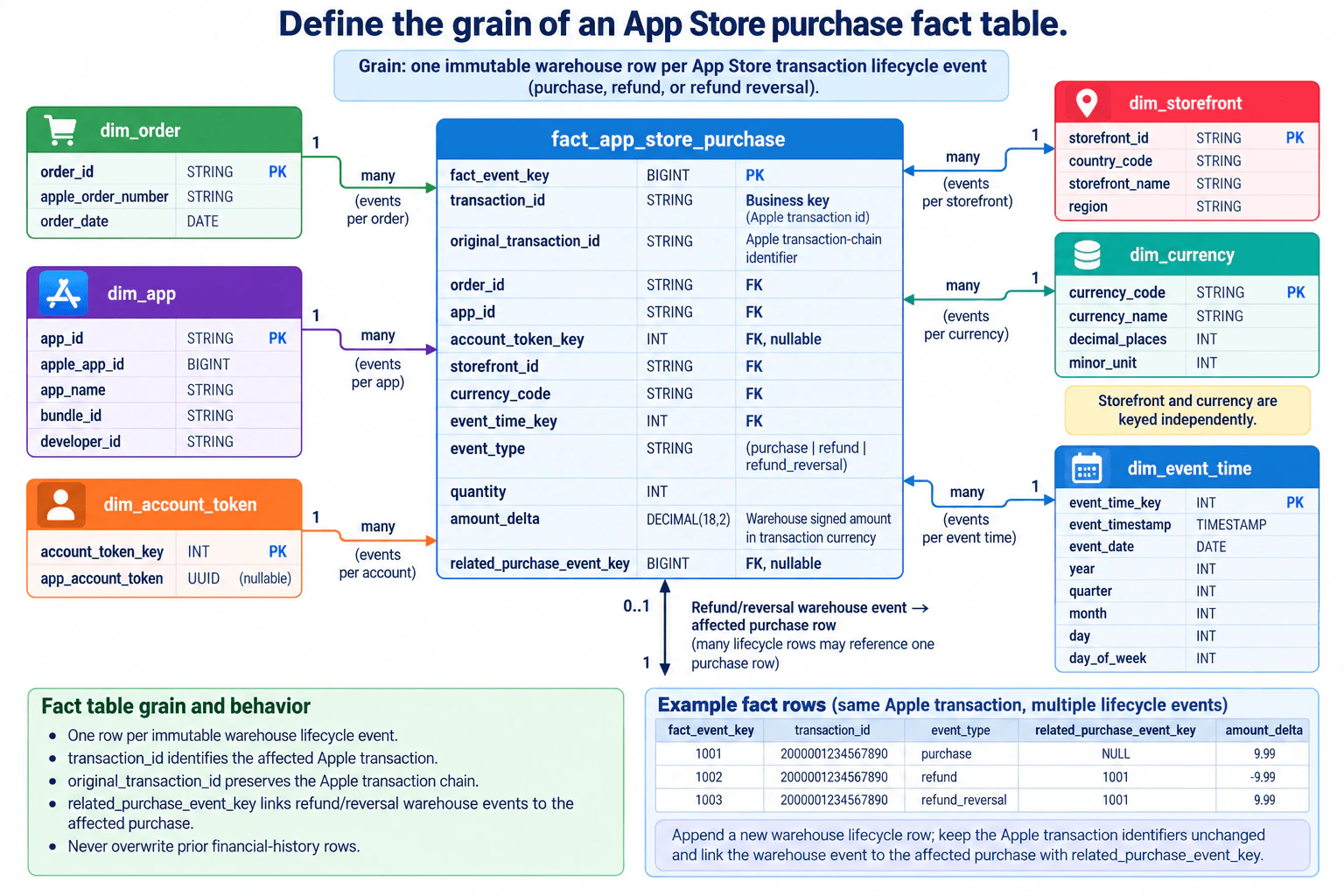
Define the grain of an App Store purchase fact table. diagram
How to Explain It in an Interview

Start by declaring the grain: one immutable row in fact_app_store_purchase represents one App Store transaction lifecycle event. The event can be a purchase, refund, or refund_reversal. Grain means exactly what one fact-table row represents.

Use fact_event_key as the warehouse primary key. It is a BIGINT surrogate key, meaning it is generated for the warehouse and uniquely identifies each stored lifecycle event. Keep transaction_id as the Apple transaction business identifier. Keep original_transaction_id separately because it preserves the Apple transaction chain; it is not the warehouse self-reference used to connect a refund or refund reversal to the affected purchase row.

Key the supporting dimensions at the same fact grain. order_id is a foreign key to dim_order.order_id. app_id is a foreign key to dim_app.app_id. account_token_key is a nullable foreign key to dim_account_token.account_token_key, where app_account_token is the optional UUID attribute. storefront_id is a foreign key to dim_storefront.storefront_id. currency_code is a foreign key to dim_currency.currency_code. Storefront and currency are keyed independently and should not be inferred from one another. event_time_key is a foreign key to dim_event_time.event_time_key, where the dimension carries event_timestamp, event_date, year, quarter, month, day, and day_of_week.

The fact also stores event_type, quantity, and amount_delta. amount_delta is a signed warehouse amount in the transaction currency. A purchase contributes a positive amount, a refund contributes a negative amount, and a refund reversal contributes the restoring positive amount. This lets downstream calculations sum lifecycle rows without modifying earlier financial records.

For refund history, use related_purchase_event_key as a nullable self-referencing foreign key to fact_app_store_purchase.fact_event_key. A purchase normally has NULL in this field. A refund or refund-reversal warehouse row points to the fact_event_key of the affected purchase. Multiple lifecycle rows may therefore reference one purchase row. This relationship is separate from original_transaction_id: related_purchase_event_key is the warehouse relationship between lifecycle rows, while original_transaction_id preserves the Apple transaction-chain identifier.

For example, suppose fact_event_key 1001 is a purchase for transaction_id 2000001234567890 with amount_delta 9.99. A later refund is fact_event_key 1002 with the same transaction_id, related_purchase_event_key 1001, and amount_delta -9.99. If that refund is reversed, fact_event_key 1003 again uses the same transaction_id, points to purchase 1001, and carries amount_delta 9.99. Nothing overwrites row 1001.

The main tradeoff is that this event-style fact stores more rows than a model that keeps only the latest state. The benefit is stronger auditability: every financial change remains visible, and net financial results can be recomputed from immutable history.

Technical Approach
  1. Declare the business process as App Store transaction lifecycle activity.
  2. Set the fact grain to one immutable warehouse row per purchase, refund, or refund-reversal event.
  3. Generate fact_event_key as the warehouse primary key while retaining transaction_id and original_transaction_id as Apple business identifiers.
  4. Resolve order_id, app_id, nullable account_token_key, storefront_id, currency_code, and event_time_key to their supporting dimensions.
  5. Store event_type, quantity, and signed amount_delta at that same event grain.
  6. For a refund or refund reversal, append a new fact row and set related_purchase_event_key to the affected purchase fact_event_key.
  7. Never update the original purchase row to represent a later financial event.
Practical Insights

Storage grows with the number of lifecycle events because refunds and reversals add rows instead of replacing earlier rows. Each new event needs dimension-key resolution and one new fact row. Reporting stays simple because signed amount_delta values can be summed, but consumers must understand the event grain. Maintenance requires consistent source identifiers, foreign keys, and related_purchase_event_key relationships. The benefit is complete financial history and straightforward auditing.

Why Interviewers Ask This

This tests whether the candidate can declare a precise fact-table grain before designing dimensions and measures, separate warehouse keys from source-system business identifiers, model dimension relationships correctly, and preserve an auditable financial history when purchases later receive refunds or refund reversals.

Common interview mistakes

Common mistakes are defining the grain as one row per order or one row per transaction regardless of later lifecycle events; overwriting the purchase when a refund arrives; treating transaction_id as the warehouse event primary key; using original_transaction_id as though it were the warehouse refund-to-purchase foreign key; making the optional app account token mandatory; joining a raw timestamp directly to a date-only key instead of using event_time_key; inferring storefront from currency; and representing refunds without a negative financial effect. Another mistake is placing descriptive dimension attributes in the fact table instead of using the corresponding dimensions.

Interview tip

State the grain first in one sentence. Then name the warehouse key, the Apple business identifiers, the six required dimension relationships, and the append-only refund relationship. Finish with the three-row purchase, refund, and refund-reversal example to show why financial history is never overwritten.
Interviewer may ask next
How would you model multiple refunds or other lifecycle events that relate to the same purchase?

Append one new fact row for each lifecycle event. Each row receives a new fact_event_key and can retain the same affected transaction_id. For events related to the purchase, related_purchase_event_key points to that purchase's fact_event_key. Because many lifecycle rows can reference one purchase, multiple later events can be stored without changing the original purchase row.

Why keep both original_transaction_id and related_purchase_event_key?

They represent different relationships. original_transaction_id is retained from Apple to preserve the Apple transaction chain. related_purchase_event_key is a warehouse foreign key that directly connects a refund or refund-reversal lifecycle row to the affected purchase fact row. Keeping both avoids confusing the source-system transaction relationship with the warehouse's own immutable event relationship.

2. Model iCloud storage usage for a real-time dashboard and weekly trends.Data ModelingEasyApple

Question Details

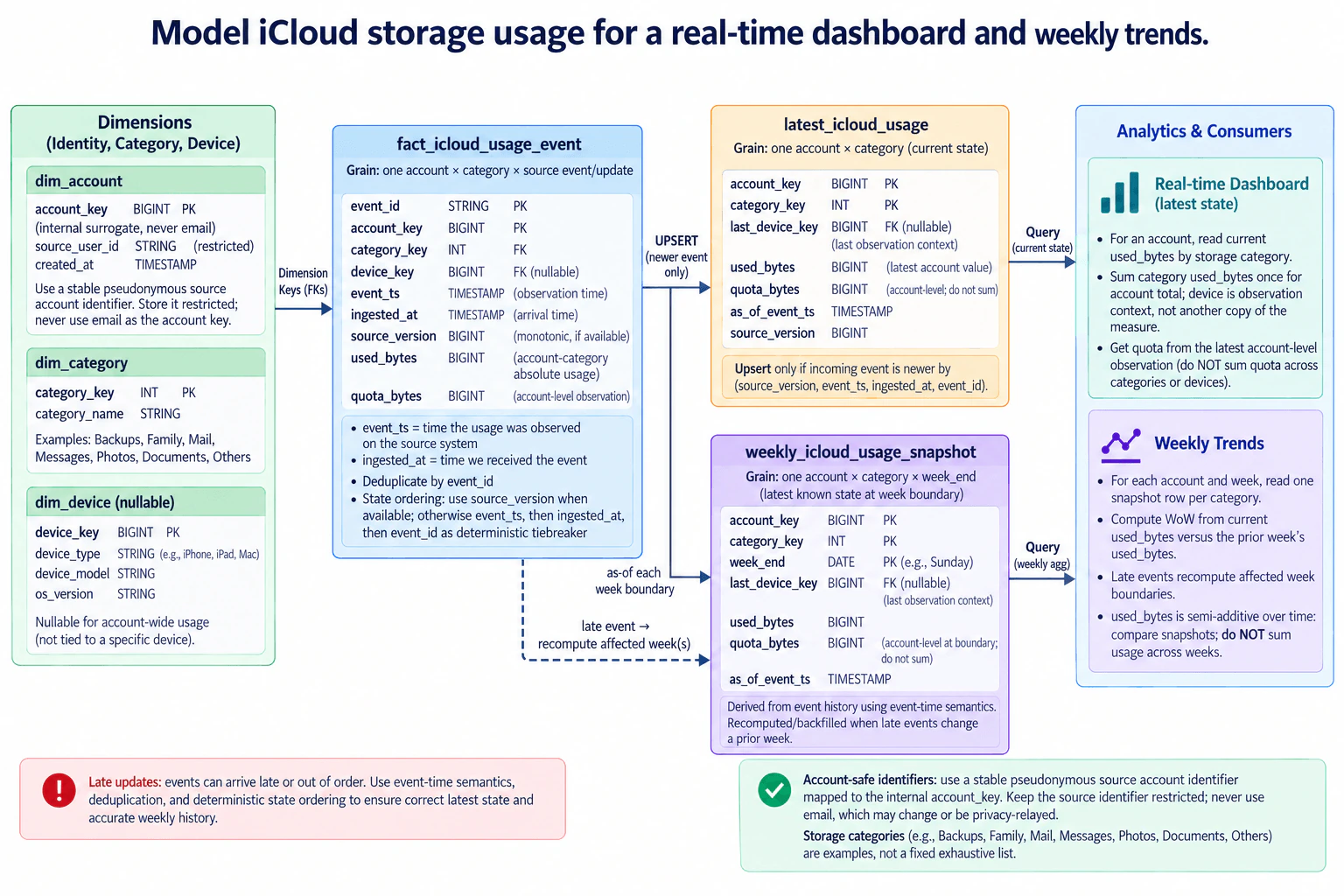
Create a schema that supports current iCloud storage usage as well as week-over-week history. Define account-safe identifiers, storage category, device context, quota and used bytes, event versus snapshot grains, late updates, and the query path for both a latest-state dashboard and weekly aggregation.

Short Interview Answer (30-60 seconds)

Store every usage observation in event history, maintain one current row per account and category, and materialize one snapshot per account, category, and week. Use pseudonymous account IDs, optional device context, non-additive quota, deterministic event ordering, and backfill affected weeks when late events arrive.

Detailed Explanation

The model needs to answer two simple questions: how much storage an account uses now, and how that amount changed from week to week. Keep every incoming observation so older periods can still be corrected. Give each account a safe internal identity instead of using email. Separate storage into categories such as Photos, Backups, Mail, Messages, Documents, Family, and Others. A device can be recorded when it supplied the observation, but the storage amount belongs to the account and category. Newer observations update the current view, while late observations can repair past weekly results.

Useful Questions to Ask the Interviewer
  1. Are used_bytes values absolute account-category usage observations rather than byte deltas?
  2. Is quota_bytes one account-level quota that may be repeated on category rows only for convenient reads?
  3. Can events arrive late or out of order, and is source_version monotonic when present?
  4. Is device information optional observation context rather than part of the storage measurement grain?
  5. What day and time zone define the weekly boundary?
Model iCloud storage usage for a real-time dashboard and weekly trends. diagram
How to Explain It in an Interview

I would separate the design into dimensions, immutable event history, a latest-state table, and a periodic weekly snapshot.

dim_account has one row per account. Its primary key is account_key BIGINT, an internal surrogate key. source_user_id STRING is the restricted pseudonymous source identifier. Email is not used as the account key. created_at TIMESTAMP records when the dimension row was created.

dim_category has one row per storage category. Its primary key is category_key INT, with category_name STRING for values such as Backups, Family, Mail, Messages, Photos, Documents, and Others.

dim_device contains optional device context. Its primary key is device_key BIGINT, with device_type STRING, device_model STRING, and os_version STRING. The relationship is optional because account-wide storage usage may not be tied to one specific device.

The immutable history table is fact_icloud_usage_event. Its grain is one account × category × source event/update. event_id STRING uniquely identifies an event. account_key BIGINT, category_key INT, and nullable device_key BIGINT reference the dimensions. event_ts TIMESTAMP is when the usage was observed at the source, while ingested_at TIMESTAMP is when the pipeline received it. source_version BIGINT is used when the producer supplies a monotonic version. used_bytes BIGINT is an absolute account-category usage observation. quota_bytes BIGINT is an account-level observation and must not be summed across categories.

I would deduplicate retries by event_id. For competing observations of the same account and category, prefer the greater source_version when a reliable monotonic version is available. Otherwise compare event_ts, then ingested_at, then event_id as a deterministic tie-breaker. This prevents an older event that arrives late from incorrectly replacing newer current state.

For the real-time dashboard, maintain latest_icloud_usage at exactly one account × category. Its composite primary key is account_key plus category_key. It stores nullable last_device_key only as observation context, plus used_bytes, account-level quota_bytes, as_of_event_ts, and source_version. Upsert the row only when the incoming event wins the ordering rule.

The dashboard reads current used_bytes by category. To calculate an account total, sum each current category value once. Do not aggregate separate device observations as though each were another copy of storage usage. Likewise, do not sum repeated quota_bytes values across categories or devices because quota is account-level.

For historical trends, maintain weekly_icloud_usage_snapshot at one account × category × week_end. The composite key is account_key, category_key, and week_end. Each row represents the latest known state at that week's boundary and stores nullable last_device_key, used_bytes, account-level quota_bytes, and as_of_event_ts.

The weekly table must be derived from event history using event-time semantics. It should not be reconstructed from today's latest-state table because today's state cannot reproduce what was known at earlier boundaries. The diagram shows Sunday only as an example week end; the production design should use one explicitly agreed week boundary and time zone.

For week-over-week analysis, read one snapshot row per account, category, and week, then compare used_bytes with the prior week's value. used_bytes is semi-additive over time: category values may be combined at the same point in time when they represent non-overlapping categories, but usage observations must not be summed across different weeks. Week-over-week analysis therefore uses differences or percentage changes between snapshots.

Late data is the important failure case. Keep the late event in the immutable history and place it according to event_ts. If it changes which observation should have been selected at a previous week boundary, recompute the affected week or weeks. The same deterministic ordering rule protects the current-state table from being overwritten by an older observation.

The main tradeoff is extra storage and maintenance work. The event table preserves complete history and supports repair. The latest-state table makes current dashboard reads small and fast. The weekly snapshot avoids repeatedly reconstructing historical state from raw events. This denormalization increases write and backfill work, but it gives predictable query paths for both real-time and historical consumers.

Technical Approach
  1. Resolve the restricted pseudonymous source identifier to dim_account.account_key, and look up the storage category and optional device keys.
  2. Append the observation to fact_icloud_usage_event and deduplicate by event_id.
  3. Determine event precedence using source_version when it is reliably monotonic; otherwise use event_ts, then ingested_at, then event_id.
  4. Upsert latest_icloud_usage only when the incoming event is newer, preserving one row per account and category.
  5. At each agreed weekly boundary, derive weekly_icloud_usage_snapshot from event history by choosing the latest valid observation for each account and category as of that boundary.
  6. When a late event changes historical ordering, recompute the affected weekly boundary or boundaries.
  7. Serve current usage from latest_icloud_usage and calculate week-over-week changes by comparing consecutive weekly snapshot rows.
Practical Insights

The raw event table grows with every observation, so its storage cost follows event volume and retention time. The current-state table stays much smaller because it keeps only one row per active account-category pair. Weekly snapshot storage grows with active account-category pairs multiplied by retained weeks. Dashboard reads are inexpensive because they use only current rows, and trend reads use periodic snapshots instead of replaying the entire history. Late events add processing cost because some historical weeks may need to be recalculated. The design also has maintenance cost because derived current and weekly tables must stay consistent with the immutable event history.

Why Interviewers Ask This

This question tests whether the candidate can separate immutable event history from current state and periodic snapshots, declare correct table grains and keys, avoid double-counting account-level measures, model optional device context, handle late and out-of-order observations, and design efficient query paths for both current dashboards and week-over-week analytics.

Common interview mistakes

Common mistakes are using email as the account identifier; treating optional device context as part of the storage measurement grain; counting the same account-category usage once per device; summing account-level quota_bytes across categories; treating absolute used_bytes observations as additive deltas; building weekly history from only the current latest-state table; using ingestion time instead of event time for historical boundaries; failing to deduplicate retries; letting an older late event overwrite newer current state; summing usage across weeks instead of comparing snapshots; and failing to recompute affected historical weeks after late arrivals.

Interview tip

Start by declaring the three grains: event history is one account-category-source update, current state is one account-category, and weekly history is one account-category-week boundary. Then explain that device is nullable context, quota is account-level, and event-time ordering plus backfills handles late data.

Interviewer may ask next
How would you handle two events for the same account and category that arrive out of order?

Keep both events in the immutable history. Deduplicate exact retries by event_id. If a reliable monotonic source_version exists, use it to decide which observation is newer. Otherwise compare event_ts, then ingested_at, then event_id as a deterministic tie-breaker. Update latest_icloud_usage only when the incoming observation wins that ordering. If a late observation changes the state that should have existed at an earlier week boundary, recompute the affected weekly snapshot rows.

Why not calculate the real-time dashboard and weekly trends directly from the raw event table?

It would be logically possible, but every dashboard request would repeatedly deduplicate and rank a growing event history, and each trend request would have to reconstruct historical state at multiple boundaries. latest_icloud_usage provides a compact current-state read path, while weekly_icloud_usage_snapshot provides a stable historical grain. The raw event table remains the durable source for auditability and late-data correction. The tradeoff is additional storage plus the operational work required to maintain and backfill the derived tables.

3. Design a ten-billion-row fact table that receives hourly updates.Data ModelingMediumApple

Question Details

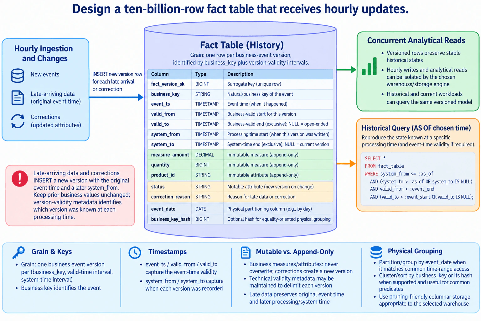
Specify the grain, business key, event and processing timestamps, mutable versus append-only attributes, and physical grouping metadata for a fact table with concurrent analytical reads and hourly changes. Include representation of late data and corrections so historical queries can reproduce the state known at a chosen time.

Short Interview Answer (30-60 seconds)

Use one row per business-event version. Keep the business key, event time, business-valid interval, and processing/system-time interval. Write a new version for late data or corrections instead of overwriting prior business values, then organize storage by event date and useful business-key predicates.

Detailed Explanation

The table must hold a huge amount of information while new changes arrive every hour. The important idea is to keep earlier versions instead of replacing them, so a report can show what was known at any chosen moment. Each event needs a stable business identifier, the time it happened, and the time each version became known. Late information keeps its original event time but gets a later recorded time. Corrections create another version. The stored data should also be organized so common time-based searches can avoid reading the full table while analytical reads continue alongside hourly writes.

Useful Questions to Ask the Interviewer
  1. Which warehouse or storage engine will hold the table?
  2. Are the most common analytical filters based on event date, business key, or both?
  3. Do historical queries need only processing-time reconstruction, or must they also apply business-valid time?
  4. How late can events arrive, and how frequently are existing events corrected?
  5. How should logical deletes be represented if they are required?
Design a ten-billion-row fact table that receives hourly updates. diagram
How to Explain It in an Interview

Start with the grain: one row represents one version of one business event. The business_key is the natural business identifier for the event. fact_version_sk is a BIGINT surrogate key that uniquely identifies each stored version row.

Keep event time and processing time separate. event_ts is the timestamp when the business event happened. valid_from and valid_to define when that version is valid in business time. Use a half-open interval: valid_from is inclusive and valid_to is exclusive. A NULL valid_to means the business-valid interval is open-ended.

system_from records the processing time when that version became known to the warehouse. system_to is the exclusive end of the processing-time interval for that version. A NULL system_to means it is the current recorded version. These system-time columns are technical version-validity metadata used to reproduce what the warehouse knew at a chosen processing time.

The schema in the approved design is: fact_version_sk BIGINT, business_key STRING, event_ts TIMESTAMP, valid_from TIMESTAMP, valid_to TIMESTAMP, system_from TIMESTAMP, system_to TIMESTAMP, measure_amount DECIMAL, quantity BIGINT, product_id STRING, status STRING, correction_reason STRING, event_date DATE, and business_key_hash BIGINT.

Treat business measures and core attributes as history that should not be overwritten. measure_amount, quantity, and product_id are represented as immutable values for a stored version. status is an example of a business attribute that may change. When it changes, create another version row instead of replacing the earlier business values. correction_reason records why a late arrival or correction was introduced.

Late-arriving data keeps its original event_ts. Because the warehouse learns about it later, its new version has a later system_from. Corrections follow the same versioning rule. Prior business values remain available, while system-time metadata identifies which version was known during each processing-time interval.

For a historical query at :as_of, select rows where system_from <= :as_of and where system_to > :as_of or system_to IS NULL. If the query also needs a business-valid event-time range, require valid_from < :event_end and valid_to > :event_start or valid_to IS NULL. These half-open interval comparisons avoid returning a version that ended exactly when the requested interval begins.

For physical organization, event_date is the partitioning or grouping column when common access patterns use event-time ranges. business_key or its hash can be used for clustering or sorting when the selected warehouse supports that feature and the workload benefits from those predicates. business_key_hash is optional physical metadata for equality-oriented grouping; it is not a universal requirement. Use pruning-friendly columnar storage suitable for the chosen analytical warehouse.

For concurrent analytical reads, the versioned rows preserve stable historical states. Hourly writes and analytical reads can be isolated by the selected warehouse or storage engine. Do not claim a specific snapshot-isolation or nonblocking guarantee without naming the engine and its transaction behavior.

The main tradeoff is storage versus reproducibility. Keeping multiple versions increases row count and storage, but it preserves the ability to reconstruct exactly what was known at an earlier processing time. Physical grouping can reduce scanned data when filters match the chosen grouping columns, but the benefit is workload- and engine-dependent.

Technical Approach
  1. Declare the grain as one row per business-event version.
  2. Use business_key as the natural event identifier and fact_version_sk as the unique surrogate row key.
  3. Store event_ts separately from system_from so event occurrence time and warehouse processing time are never confused.
  4. Represent business-time validity with valid_from and valid_to using inclusive-start, exclusive-end semantics.
  5. Represent processing-time validity with system_from and system_to using the same half-open interval convention.
  6. Insert a new version when late data or a correction arrives instead of overwriting prior business values.
  7. Keep the original event time for late data and assign the later processing time to system_from.
  8. Use correction_reason to describe why the new version exists.
  9. Partition or group by event_date when common analytical filters benefit from time pruning.
  10. Cluster or sort by business_key or its hash only when the selected warehouse supports it and the access pattern benefits.
  11. Reconstruct historical state by selecting the row version whose system-time interval contains the requested as-of timestamp.
Practical Insights

The biggest cost is extra storage because one business event can have several versions. Hourly writes scale with the number of new events, late arrivals, and corrections received during that hour. Historical queries may examine more rows than a current-state-only model, but event-date pruning and useful clustering or sorting can reduce the amount of data read when query filters match those fields. Maintenance includes managing physical partitions or groups, monitoring version growth, and keeping temporal metadata consistent. At ten-billion-row scale, exact scan, write, concurrency, and maintenance costs depend on the chosen warehouse and its storage engine.

Why Interviewers Ask This

This tests whether the candidate can design a very large analytical fact table that accepts frequent changes without losing history. The interviewer wants to see a precise grain, sensible business and surrogate keys, separation of event time from processing time, correct version handling for late data and corrections, reproducible point-in-time queries, and practical physical organization for concurrent analytical workloads.

Common interview mistakes

Common mistakes include defining the grain as one row per business event while storing multiple versions without explicitly changing the grain; using only event_ts and losing the distinction between event time and processing time; overwriting corrected business values and destroying history; using only an is_current flag for historical reconstruction; assigning a late event's processing time as its event time; using inclusive end boundaries that can double-count adjacent validity intervals; failing to store the system-time interval needed for point-in-time reconstruction; assuming business_key_hash must always be the clustering key; claiming that partitioning or clustering always improves performance; and claiming that hourly writes never block readers without specifying the warehouse engine and isolation behavior.

Interview tip

Lead with the grain, then explain the two time axes. Say that late data and corrections create new versions instead of overwriting prior business values. Show the half-open as-of predicate next, then finish with event-date grouping and workload-dependent clustering as physical design choices rather than universal guarantees.

Interviewer may ask next
How would you reproduce exactly what the warehouse knew at a chosen processing time?

Use the system-time interval for each version. A row is visible at :as_of when system_from <= :as_of and either system_to > :as_of or system_to IS NULL. If the query also has a business-valid event-time range, require valid_from < :event_end and either valid_to > :event_start or valid_to IS NULL. Because earlier versions are retained, a version that was corrected later can still be returned for an earlier processing time.

What happens when late data or a correction belongs to an old event_date partition or physical group?

Keep the original event_ts and event_date semantics because they describe when the event happened. Insert the new version with a later system_from and retain the prior business values. The logical history remains correct even though the new version belongs to an older event-time grouping. The operational cost of writing, compacting, or reorganizing that older physical group depends on the selected warehouse, so that behavior should be tested against the actual engine and workload.

4. Model Apple Search ranking results and judgments for NDCG analysis.Data ModelingHardApple

Question Details

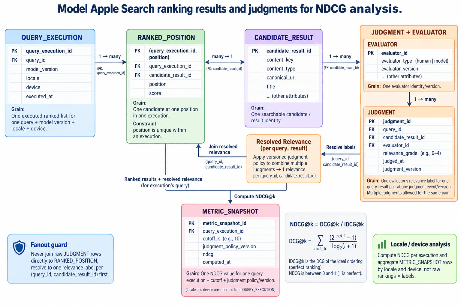
One query may produce multiple ranked result lists from different model versions and may receive multiple human or model judgments per result. Design keys and grains for query execution, ranked position, candidate result, judgment, evaluator, and metric snapshot so NDCG by locale and device is computed without multiplying rankings or labels.

Short Interview Answer (30-60 seconds)

Model executions, ranked positions, candidate results, evaluators, judgments, and metric snapshots separately. Resolve multiple judgments to one relevance value per query-result pair before joining to ranked positions. Compute NDCG per execution and cutoff, then aggregate those snapshots by locale and device.

Detailed Explanation

The main problem is keeping several versions of a search ranking separate from several opinions about the same result. One search can run with different ranking versions, and the same result can receive many reviews. If all of those rows are joined together directly, the data can be counted more than once and the final score becomes wrong. The design therefore gives each executed ranking its own identity, keeps each result as a reusable identity, stores every review separately, combines reviews once per query and result, and saves the final score at a clear level for later comparison by locale and device.

Useful Questions to Ask the Interviewer
  1. Can the same logical query have multiple query executions for different model versions, locales, devices, or execution times?
  2. What policy should combine multiple human or model judgments for the same query-result pair: average, weighted average, adjudication, or another deterministic rule?
  3. Which NDCG cutoffs must be supported, such as NDCG@10, and should several cutoffs be stored for one execution?
  4. Must candidate_result_id be unique within a query execution, in addition to position being unique?
  5. How should missing judgments be handled before an NDCG snapshot is considered valid?
Model Apple Search ranking results and judgments for NDCG analysis. diagram
How to Explain It in an Interview

Start by declaring the grain of every table because grain is what prevents accidental duplication.

QUERY_EXECUTION has one row for one executed ranked list. Its primary key is query_execution_id. It also carries query_id, model_version, locale, device, and executed_at. The same logical query can therefore have many executions for different model versions or execution contexts.

RANKED_POSITION has one row for one candidate at one position in one execution. The diagram uses the composite primary key (query_execution_id, position). It also stores query_execution_id as a foreign key, candidate_result_id as a foreign key, position, and score. QUERY_EXECUTION therefore has a one-to-many relationship with RANKED_POSITION, and each position is unique within an execution.

CANDIDATE_RESULT has one row for one searchable result identity. candidate_result_id is its primary key. Descriptive fields such as content_key, content_type, canonical_url, and title live here so the same result identity can be reused across many ranking executions.

EVALUATOR has one row for one evaluator identity and version. evaluator_id is the primary key. evaluator_type identifies whether the evaluator is human or model based, and evaluator_version records its version.

JUDGMENT has one row for one evaluator's relevance label for one query-result pair at one judgment event or version. judgment_id is the primary key. It references query_id, candidate_result_id, and evaluator_id and stores relevance_grade, judged_at, and judgment_version. Multiple judgments are allowed for the same query-result pair.

The key modeling choice is that JUDGMENT does not point to RANKED_POSITION. A relevance judgment belongs to the logical query-result pair, while a ranked position belongs to one particular query execution. That lets the same judgment set support comparisons across several model-version ranking executions.

Before computing NDCG, apply a versioned judgment policy that reduces the raw JUDGMENT rows to exactly one resolved relevance value for each (query_id, candidate_result_id). The policy could use averaging, weighting, adjudication, or another deterministic rule. The important point is that the policy is explicit and versioned.

Next, join the resolved relevance rows to RANKED_POSITION using candidate_result_id together with the query_id obtained through QUERY_EXECUTION. Because the judgments have already been reduced to one row per query-result pair, this join preserves the ranked-position grain instead of multiplying rows.

For cutoff k, compute DCG from the ranked positions using the resolved relevance grades. The diagram uses the gain term 2^rel - 1 and the discount log2(position + 1). Compute IDCG from the same resolved relevance values placed in ideal descending relevance order. Then calculate NDCG@k as DCG@k divided by IDCG@k. If IDCG is zero, the metric contract must define how that case is represented rather than performing an unchecked division by zero.

METRIC_SNAPSHOT stores one NDCG value for one query execution, cutoff, and judgment-policy version. metric_snapshot_id is the primary key, and query_execution_id is a foreign key. It also stores cutoff_k, judgment_policy_version, ndcg, and computed_at. Locale and device are inherited from QUERY_EXECUTION rather than duplicated into the metric snapshot.

For locale and device analysis, first compute NDCG independently for each query execution. Then join METRIC_SNAPSHOT back to QUERY_EXECUTION and aggregate those snapshot rows by locale and device. Do not join raw JUDGMENT rows directly to raw RANKED_POSITION rows because multiple judgments for the same result would duplicate ranked rows and distort DCG.

The tradeoff is that this design uses several normalized entities and requires an explicit relevance-resolution step. In return, each table has one clear grain, judgments remain reusable across model versions, metric computation avoids fan-out, and saved NDCG snapshots remain reproducible through their judgment-policy version.

Technical Approach
  1. Create one QUERY_EXECUTION row for every produced ranked list, carrying query_id, model_version, locale, device, and executed_at.
  2. Store each ranked candidate in RANKED_POSITION at the grain of one candidate at one position in one execution, linked to CANDIDATE_RESULT.
  3. Store each stable searchable result identity once in CANDIDATE_RESULT.
  4. Store each human or model evaluator identity/version in EVALUATOR.
  5. Store every relevance label in JUDGMENT at the grain of one evaluator's label for one query-result pair at one judgment event/version.
  6. Apply judgment_policy_version to reduce multiple labels to exactly one relevance value per (query_id, candidate_result_id).
  7. Join those resolved relevance values to the ranked positions for the matching execution query and candidate, preserving one row per ranked position.
  8. For each cutoff k, calculate DCG from the actual ranked positions and IDCG from the same resolved labels in ideal relevance order, then derive NDCG.
  9. Store the result in METRIC_SNAPSHOT at one row per query execution, cutoff, and judgment-policy version.
  10. Analyze by locale and device by joining METRIC_SNAPSHOT to QUERY_EXECUTION and aggregating snapshot rows rather than raw ranking-label rows.
Practical Insights

Storage grows with the number of query executions, ranked positions, candidate results, evaluators, judgments, and saved metric snapshots. For k evaluated positions, DCG requires work proportional to k. Building IDCG by sorting the resolved relevance values is typically O(k log k). The main data-processing cost is resolving potentially many judgment rows before metric computation. The normalized design introduces joins and policy-version maintenance, but it prevents incorrect fan-out and keeps the metric reproducible.

Why Interviewers Ask This

This question tests whether the candidate can declare precise table grains, choose stable keys, model one-to-many relationships, prevent many-to-many fan-out, separate reusable judgments from execution-specific rankings, and define a reproducible NDCG metric at the correct aggregation level.

Common interview mistakes

A common mistake is attaching JUDGMENT directly to RANKED_POSITION, which makes a reusable relevance label depend on one execution-specific ranking row. Another mistake is joining all raw JUDGMENT rows directly to RANKED_POSITION, causing one ranked row to appear once per evaluator. Other mistakes include mixing candidate identity with ranked position, failing to version the judgment-resolution policy, computing locale/device aggregates before computing per-execution NDCG, calculating IDCG from a different relevance set than DCG, ignoring zero-IDCG behavior, or duplicating locale and device into several tables without a clear owner.

Interview tip

Lead with the grain of each table and then call out the fan-out risk. The key sentence is: resolve many judgments to one relevance value per query-result pair before joining them to execution-specific ranked positions. Finish by showing that NDCG is stored per execution and only then aggregated by locale and device.

Interviewer may ask next
How would you handle several human and model judgments for the same query-result pair?

Keep every judgment as its own JUDGMENT row with evaluator_id, relevance_grade, judged_at, and judgment_version. Apply a deterministic, versioned judgment policy before joining to ranking rows, producing exactly one resolved relevance value per (query_id, candidate_result_id). Store the policy version with METRIC_SNAPSHOT so the NDCG value can be reproduced after the policy changes.

What happens if a ranked result has no resolved judgment?

Define the metric contract explicitly instead of relying on an accidental join result. One policy may require all evaluated positions to have usable judgments before computing the snapshot; another may map missing relevance to a documented default such as zero. Whichever rule is chosen must be part of the versioned judgment policy and must be applied consistently when constructing both DCG and the corresponding IDCG.

5. Design a daily clickstream batch ingestion flow with late events.Data PipelinesEasyApple

Question Details

Build a daily pipeline for clickstream files that may be retried or arrive after the nominal partition closes. Specify landing layout, partition discovery, deduplication identity, transformation checkpoints, idempotent publication, and the rule for reopening or correcting a previously completed date.

Short Interview Answer (30-60 seconds)

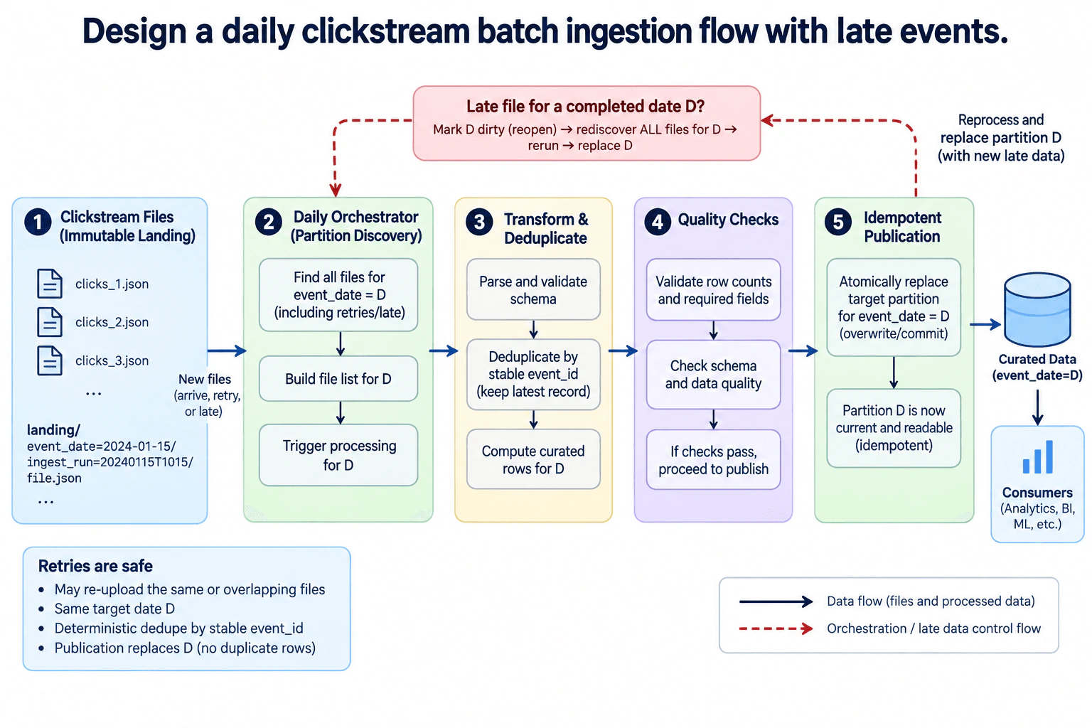
I would land every clickstream file immutably by event date and ingestion run. For date D, the orchestrator discovers all files, including retries and late arrivals, then parses, validates, and deduplicates records by stable event_id. After row-count, required-field, schema, and quality checks pass, I atomically replace the curated partition for D. If a late file arrives later, I reopen D, rediscover all files, rerun deterministically, and replace D again. The trade-off is extra reprocessing in exchange for simpler correctness.

Detailed Explanation

The goal is to build one daily process that turns click files into a trustworthy daily dataset. Files can arrive more than once or can arrive after a day was already considered finished. The process must therefore know which day each file belongs to, avoid counting the same event twice, check the data before making it available, and safely correct an older day when new files appear. The key idea is that repeating the work for a date should produce the same correct daily result instead of adding another copy of the data.

Useful Questions to Ask the Interviewer
  1. Does every click event have a stable event_id that stays the same when a file is retried?
  2. How should we determine that a late file belongs to an already completed event date?
  3. Is replacing the complete curated partition for one date acceptable when that date is reopened?
  4. Which row-count, required-field, schema, and data-quality checks must block publication?
Design a daily clickstream batch ingestion flow with late events. diagram
How to Explain It in an Interview
1. Land clickstream files immutably

I would start by keeping every received clickstream file unchanged in the landing area. The diagram organizes files under an event-date partition and an ingestion-run path, such as landing/event_date=2024-01-15/ingest_run=20240115T1015/file.json. Because landing is immutable, a retry can add the same or an overlapping file without destroying earlier input. This gives the pipeline a reproducible source for reruns. The landing area stores the business data, while the orchestrator only discovers files and coordinates processing.

2. Discover the complete input for date D

The Daily Orchestrator performs partition discovery. For target date D, it finds all files for D, including files that were retried or arrived late. It builds the complete file list and triggers processing for that date. A correction run must not process only the newest late file. It rediscovers the full input set for D so the same transformation logic can rebuild the complete result deterministically.

3. Transform and deduplicate

The processing stage first parses each file and validates its schema. It then deduplicates records using the stable event_id shown in the diagram and keeps one latest record for each event identity. This separates file-delivery behavior from business-result correctness. Duplicate or overlapping files may exist in immutable landing, but they should not create duplicate curated events. After deduplication, the pipeline computes the curated rows for D. Repeating the processing therefore repeats work without intentionally creating additional business rows.

4. Gate publication with quality checks

The computed rows are not published immediately. The Quality Checks stage validates row counts and required fields, then checks schema and data quality. Only when those checks pass does the flow continue to publication. This is important because task completion alone does not prove that the produced data is correct. The diagram does not define a quarantine path or numeric quality threshold, so I would not invent one. If validation fails, the candidate replacement for D must not become the current readable curated partition.

5. Publish date D idempotently

The Idempotent Publication stage atomically replaces the target partition for event_date=D using the overwrite or commit boundary shown in the diagram. Consumers should move from the previous complete partition to the new complete partition rather than seeing a partially replaced date. Once publication completes, partition D is current and readable. Repeating the same successful run and replacing D again does not append another copy of the partition, so publication is idempotent at the date-partition boundary.

6. Reopen a completed date for late data

Late data follows the separate dashed orchestration control flow. If a file arrives for date D after D was completed, the orchestrator marks D dirty and reopens it. It then rediscovers all files for D, rebuilds the file list, reruns parsing, schema validation, event_id deduplication, curated-row computation, and quality checks, and replaces partition D again. The benefit is predictable recovery and retry behavior. The downside is extra read and compute work because the whole affected date is rebuilt even when only a small amount of late data arrived.

Technical Approach
  1. Store every incoming clickstream file unchanged in immutable landing storage under its event_date and ingest_run path.
  2. For target date D, discover all files for D, including retry and late-arriving files.
  3. Build the complete file list and trigger processing for D.
  4. Parse the files and validate their schema.
  5. Deduplicate records by stable event_id and keep one latest record per event identity.
  6. Compute the curated rows for D.
  7. Run row-count, required-field, schema, and data-quality checks.
  8. If the checks pass, atomically replace or commit the complete curated event_date=D partition.
  9. If a late file arrives after D is complete, mark D dirty, rediscover all files for D, rerun the same deterministic flow, and replace D again.
Practical Insights

The benefit is simple correctness. Reprocessing all files for one date and replacing the whole curated partition makes retries and late corrections easy to reason about. If a file is uploaded twice, stable event_id deduplication prevents duplicate business rows. The downside is extra work: reopening an older date means reading, transforming, validating, and publishing that date again even when only one new file arrived. Immutable landing also retains files from multiple ingestion runs. We accept this because a daily batch design favors predictable recovery over more complicated incremental correction logic. Strong validation may delay publication, but it protects consumers from incomplete or invalid results. The main processing cost grows with the amount of data that must be rebuilt for an affected date.

Why Interviewers Ask This

This question tests whether a candidate can design a simple batch pipeline that remains correct when files are duplicated, retried, or late. The interviewer wants to see clear separation between landing, orchestration, transformation, validation, and publication. It also tests whether the candidate understands stable deduplication identity, safe reruns, partition-level idempotency, quality gates, and how to correct an already published date without creating duplicate business results.

Common interview mistakes

Common mistakes are appending every retry directly into the curated dataset, deduplicating only by filename instead of stable event_id, processing only the newest late file instead of rebuilding the complete input for D, and treating task completion as proof that the data is valid. Another mistake is replacing a completed date without a clear publication boundary, which can expose an incomplete result. Candidates also sometimes confuse source delivery with business correctness: duplicate files may exist in immutable landing as long as deterministic deduplication and idempotent partition replacement prevent duplicate curated rows.

Interview tip

Explain the design around one invariant: rerunning date D must produce one correct partition for D. Walk left to right through immutable landing, complete partition discovery, event_id deduplication, quality gating, and atomic replacement. Then explain the dashed late-data control flow separately: mark D dirty, reopen it, rediscover all files, rerun, and replace D. That keeps the reliability story easy to follow.

Interviewer may ask next
What would you change if late files frequently arrived for dates that were already completed?

I would keep the same correctness model but make reopening completed dates a routine orchestration path rather than a rare exception. The changed requirement is recovery frequency. The Daily Orchestrator would identify completed dates that receive new files and mark each affected date D dirty. For every dirty date, it would still rediscover all files for D, rebuild the complete file list, parse and validate the input, deduplicate by stable event_id, compute the curated rows, run the same quality checks, and atomically replace the curated partition for D. I would keep the immutable landing layout and the existing processing stages unchanged. Correctness remains intact because repeated source delivery is absorbed by deterministic deduplication and publication remains idempotent at the date-partition boundary. Recovery is verified by the same row-count, required-field, schema, and data-quality gates before replacement. The main downside is additional read and compute work because frequently changing dates may be rebuilt many times.

How would you handle a processing failure after transformation starts but before the curated partition is published?

I would rerun the affected date from immutable landing data and keep the currently readable curated partition unchanged until a complete replacement passes validation. The changed requirement is failure recovery, not the architecture. The orchestrator rebuilds the full file list for D and repeats parsing, schema validation, event_id deduplication, curated-row computation, and quality checks. Any incomplete result from the failed attempt must not become the current consumer-visible partition because publication happens only at the final replacement boundary. When the rerun passes validation, the pipeline atomically replaces event_date=D, and the new partition becomes current and readable. Stable deduplication and whole-partition replacement make the rerun safe even if source files were retried. Recovery is verified with the same row-count, required-field, schema, and data-quality checks. The downside is duplicated compute for the failed attempt and the rerun, but the design avoids exposing incomplete curated data.

6. Clean a large CSV stream with missing values and duplicate records.Data PipelinesEasyApple

Question Details

Process the file incrementally rather than loading it all at once. Define parsing and type rules, required-field handling, duplicate identity, deterministic survivor selection, bounded state, rejected-row output, and an example checkpoint that permits a failed run to resume without emitting the same cleaned row twice.

Short Interview Answer (30-60 seconds)

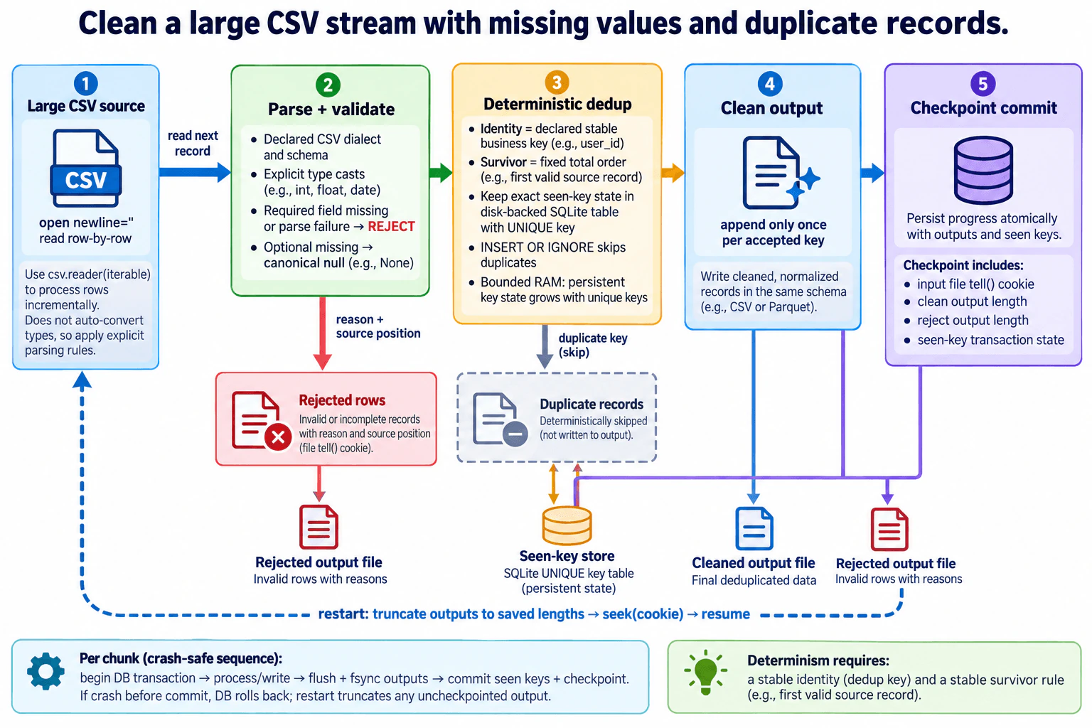
I would read the CSV incrementally, validate and normalize each row, quarantine bad rows, and deduplicate valid rows with a stable business key and a deterministic first-valid-record rule. I would store seen keys in durable disk-backed state. After each crash-safe unit, I would flush the outputs and commit the input position, output lengths, and seen-key state together. On restart, I would truncate uncommitted output and resume from the saved position. The trade-off is extra state and checkpoint I/O for reliable recovery.

Detailed Explanation

See the Code while reading this explanation.

This question asks us to clean a very large file without putting the whole file in memory. Each row must be checked and converted into the expected form. Bad or incomplete rows must be kept separately instead of disappearing. Repeated records must produce only one final row, using the same rule every time. The process must also remember its last safe point. If it stops unexpectedly, it should remove unfinished output and continue from that point instead of starting over or writing the same accepted row again.

Useful Questions to Ask the Interviewer
  1. Which columns are required, and what type should each column have?
  2. What field or field combination identifies a duplicate record?
  3. If duplicate rows differ, which one should survive: first valid row, latest row, or another deterministic rule?
  4. How should optional missing values be represented in the cleaned output?
  5. Which CSV dialect, quoting rules, encoding, and date formats should be accepted?
  6. Should rejected rows keep the original row, error reason, and source position?
Clean a large CSV stream with missing values and duplicate records. diagram
How to Explain It in an Interview
1. Read the large CSV incrementally

I would treat the CSV as a sequential file source and read it record by record rather than loading the complete dataset. The diagram uses Python's CSV reader with an explicit dialect and newline="". That keeps working memory bounded by the current record or small processing unit. The reader returns strings, so the pipeline applies the real data contract explicitly instead of relying on automatic type inference.

2. Parse, normalize, and reject bad rows

For each record, I would apply declared type parsers and required-field rules. A required field that is missing, or a value that cannot be converted to its declared type, goes to the rejected-row output. The rejected record includes the source position and an error reason so it can be investigated later. Optional blanks become one canonical null representation. This makes downstream behavior deterministic and prevents silent loss of malformed data.

3. Deduplicate with durable state

Next I would compute the declared business key, such as the diagram's example user_id. The survivor rule must be deterministic; the diagram uses the first valid source record. I would keep exact seen-key state in a disk-backed SQLite table with a UNIQUE key. A new key is inserted and its cleaned row may be written. A key that already exists is a duplicate and is skipped. This keeps RAM bounded even though persistent state grows with the number of unique keys.

4. Append accepted rows to the clean output

Only rows that pass validation and win deduplication are appended to the cleaned output, using one normalized schema. Invalid rows go to the rejected output, while duplicate valid rows are skipped. The diagram allows a cleaned CSV or another file representation such as Parquet; the important rule is that a committed deduplication key maps to one accepted business result.

5. Commit a crash-safe checkpoint

The checkpoint ties source progress to output progress and deduplication state. For each crash-safe unit, begin the SQLite transaction, process the record or bounded group, write accepted or rejected output, flush and fsync both output files, then update the checkpoint and commit the seen-key changes in the same SQLite transaction. The checkpoint records the source file's own tell() cookie plus the committed byte lengths of the clean and rejected files. Progress never advances before the corresponding output is durable.

6. Recover without duplicating cleaned rows

If the process crashes before the SQLite commit, the seen-key and checkpoint changes roll back. The files may still contain bytes written by that failed attempt, so restart first truncates both outputs to their saved lengths. It then seeks the unchanged source file to the saved position and replays from there. Because uncommitted seen keys were rolled back and uncommitted output was removed, replay does not leave a second committed cleaned row. The trade-off is extra disk I/O and persistent state, but the recovery behavior is explicit and deterministic.

Key Insight / Why This Solution Works
  1. Open the CSV for incremental reading with the declared dialect, encoding, and quoting rules.
  2. Apply explicit field parsers and normalize optional blanks to one canonical null representation.
  3. If a required field is missing or parsing fails, append the original row, error reason, and source position to the rejected output.
  4. Compute the declared stable deduplication key for each valid row.
  5. Apply the deterministic survivor rule, such as first valid source record wins.
  6. Store seen keys in a durable SQLite table with a UNIQUE or PRIMARY KEY constraint; skip keys already committed.
  7. Append each accepted survivor to the cleaned output using the normalized schema.
  8. For each crash-safe unit, start the SQLite transaction before changing seen-key state.
  9. Flush and fsync both output files, then save the next source-position cookie and the committed byte lengths of both outputs in the checkpoint and commit the SQLite transaction.
  10. After failure, roll back uncommitted SQLite state, truncate both outputs to their saved lengths, seek to the checkpointed source position, and resume.
Code
import csv
import json
import os
import sqlite3
from pathlib import Path

SOURCE = Path("input.csv")
CLEAN = Path("clean.csv")
REJECTS = Path("rejected.csv")
STATE_DB = Path("pipeline_state.sqlite")


class ReadlineIterator:
    """Feed csv.reader with readline() so TextIOWrapper.tell() stays usable."""

    def __init__(self, file_obj):
        self.file_obj = file_obj

    def __iter__(self):
        return self

    def __next__(self):
        line = self.file_obj.readline()
        if line == "":
            raise StopIteration
        return line


def parse_and_validate(row, required_fields, type_rules):
    """Apply the caller-supplied data contract and canonicalize optional blanks."""
    cleaned = {
        key: (value.strip() if isinstance(value, str) else value) for key, value in row.items()
    }

    # Empty optional values become one canonical in-memory null.
    for key, value in list(cleaned.items()):
        if value == "":
            cleaned[key] = None

    # Missing required fields and failed type conversions are rejected.
    for field in required_fields:
        if cleaned.get(field) is None:
            raise ValueError(f"missing required field: {field}")

    for field, parser in type_rules.items():
        value = cleaned.get(field)
        if value is not None:
            try:
                cleaned[field] = parser(value)
            except (TypeError, ValueError) as exc:
                raise ValueError(f"invalid {field}: {value!r}") from exc

    return cleaned


def open_state():
    db = sqlite3.connect(STATE_DB)

    # A UNIQUE business key gives exact, durable deduplication state.
    db.execute("CREATE TABLE IF NOT EXISTS seen_keys (dedup_key TEXT PRIMARY KEY)")

    # The checkpoint and seen-key changes commit in the same SQLite transaction.
    db.execute(
        "CREATE TABLE IF NOT EXISTS checkpoint ("
        "id INTEGER PRIMARY KEY CHECK (id = 1), "
        "input_cookie TEXT NOT NULL, "
        "clean_len INTEGER NOT NULL, "
        "reject_len INTEGER NOT NULL)"
    )
    db.execute(
        "INSERT OR IGNORE INTO checkpoint(id, input_cookie, clean_len, reject_len) "
        "VALUES (1, '0', 0, 0)"
    )
    db.commit()
    return db


def restore_outputs(db):
    cookie_text, clean_len, reject_len = db.execute(
        "SELECT input_cookie, clean_len, reject_len FROM checkpoint WHERE id = 1"
    ).fetchone()

    # Remove any file bytes written after the last committed checkpoint.
    for path, length in ((CLEAN, clean_len), (REJECTS, reject_len)):
        path.touch(exist_ok=True)
        with path.open("r+b") as file_obj:
            file_obj.truncate(length)

    return int(cookie_text)


def run(required_fields, dedup_key, type_rules):
    """Process one unchanged CSV source using the supplied contract."""
    db = open_state()
    saved_cookie = restore_outputs(db)

    with SOURCE.open("r", newline="", encoding="utf-8") as src:
        # Read the header once; checkpoints always point to data-record boundaries.
        header_reader = csv.reader(ReadlineIterator(src))
        fieldnames = next(header_reader)
        header_end_cookie = src.tell()
        start_cookie = header_end_cookie if saved_cookie == 0 else saved_cookie
        src.seek(start_cookie)

        # Supply the original field names explicitly when resuming mid-file.
        reader = csv.DictReader(
            ReadlineIterator(src),
            fieldnames=fieldnames,
        )

        with (
            CLEAN.open("a", newline="", encoding="utf-8") as clean_file,
            REJECTS.open("a", newline="", encoding="utf-8") as reject_file,
        ):
            clean_writer = csv.DictWriter(clean_file, fieldnames=fieldnames)
            reject_writer = csv.writer(reject_file)

            while True:
                # The readline-based iterator keeps tell() usable at CSV record boundaries.
                record_start = src.tell()
                try:
                    row = next(reader)
                except StopIteration:
                    break
                next_cookie = src.tell()

                db.execute("BEGIN")
                try:
                    try:
                        cleaned = parse_and_validate(
                            row,
                            required_fields=required_fields,
                            type_rules=type_rules,
                        )
                    except ValueError as exc:
                        # Rejected rows retain source position, reason, and original values.
                        reject_writer.writerow([str(record_start), str(exc), json.dumps(row)])
                    else:
                        key_value = cleaned.get(dedup_key)
                        if key_value is None:
                            raise ValueError(f"deduplication key is missing: {dedup_key}")

                        # First valid source record wins; later committed keys are skipped.
                        inserted = db.execute(
                            "INSERT OR IGNORE INTO seen_keys(dedup_key) VALUES (?)",
                            (str(key_value),),
                        ).rowcount

                        if inserted:
                            # Write the clean header only when committed output is empty.
                            if clean_file.tell() == 0:
                                clean_writer.writeheader()
                            clean_writer.writerow(cleaned)

                    # Make both output files durable before advancing committed progress.
                    clean_file.flush()
                    reject_file.flush()
                    os.fsync(clean_file.fileno())
                    os.fsync(reject_file.fileno())

                    clean_len = os.fstat(clean_file.fileno()).st_size
                    reject_len = os.fstat(reject_file.fileno()).st_size

                    # Commit the next source position with the matching seen-key state.
                    db.execute(
                        "UPDATE checkpoint "
                        "SET input_cookie=?, clean_len=?, reject_len=? "
                        "WHERE id=1",
                        (str(next_cookie), clean_len, reject_len),
                    )
                    db.commit()
                except Exception:
                    # SQLite state rolls back; restart truncates uncommitted file bytes.
                    db.rollback()
                    raise

    db.close()
Why Interviewers Ask This

This question tests whether a candidate can turn simple file cleaning into a reliable data pipeline. Interviewers want to see judgment around incremental processing, explicit parsing rules, required fields, duplicate identity, deterministic results, persistent state, rejected records, and crash recovery. The key skill is reasoning about what happens when work is partially written and then retried, so the final cleaned data is neither silently lost nor duplicated.

Common interview mistakes

Common mistakes are loading the whole file into memory, depending on automatic type inference, silently dropping malformed rows, and failing to distinguish required fields from optional missing values. Another mistake is using a vague duplicate identity or a survivor rule that depends on nondeterministic processing order. Keeping every seen ID in an in-memory set breaks the bounded-memory and crash-recovery requirements. A serious reliability bug is advancing the checkpoint before the matching output is durable. It is also incorrect to resume a csv.DictReader at a saved data-row position without supplying the original header, because that resumed row can be mistaken for field names. Finally, replay must remove uncheckpointed output before processing those source rows again.

Interview tip

Lead with three ideas: incremental reading, deterministic persistent deduplication, and a checkpoint tied to output state. Walk one record through validation, reject-or-accept handling, deduplication, and output. Then explain the failure window: uncommitted seen keys roll back, uncheckpointed file bytes are truncated, the source seeks to the saved position, and the same records are replayed safely. That shows business-result correctness rather than just CSV parsing.

Interviewer may ask next
What would you change if the CSV contained hundreds of millions of unique keys and the local seen-key database became the main bottleneck?

I would keep the same correctness contract but change the transaction size and how the durable key state is operated. The requirement that changes is scale: key lookups, inserts, and state-store growth now dominate processing time. The affected component is the seen-key store, not the validation rules, rejected-row path, cleaned-output contract, or recovery model.

I would process a bounded group of records per SQLite transaction and batch key operations where practical. The output for that group would still be flushed and synchronized before the checkpoint and seen-key changes commit. The checkpoint would advance only to the end of the fully committed group. On failure, restart would still truncate clean and rejected outputs to their saved lengths and replay from the previous source-position cookie.

The benefit is fewer commits and better throughput. The downside is a larger replay window after a crash and a larger amount of temporary work before each commit. I would choose a bounded group size based on state-store throughput and acceptable recovery time.

What happens if the process crashes after writing a cleaned row but before committing the checkpoint?

That row must be treated as uncommitted. The requirement that matters is idempotent recovery across a partial write. In this design, the clean file may contain bytes from the failed attempt, but the SQLite transaction containing the matching seen key and checkpoint has not committed.

On restart, SQLite exposes only the previous committed checkpoint. The pipeline reads the saved clean-output and rejected-output lengths and truncates both files back to those exact byte boundaries. It then seeks the unchanged source file to the saved input-position cookie and processes those rows again. Because the failed SQLite transaction rolled back, the corresponding seen key is also absent, so the valid survivor can be inserted and written normally during replay.

The validation and deduplication rules do not change. The downside is that some work is repeated after failure, but that bounded replay is safer than advancing progress early and risking a missing or duplicate business result.

7. Design a near-real-time Apple Search latency and quality pipeline with delayed events.Data PipelinesMediumApple

Question Details

Two to five percent of events arrive more than thirty minutes late. Define event-time windows, watermark policy, durable raw retention, provisional aggregates, late corrections, deduplication, and how dashboards distinguish stable results from values that may still change.

Short Interview Answer (30-60 seconds)

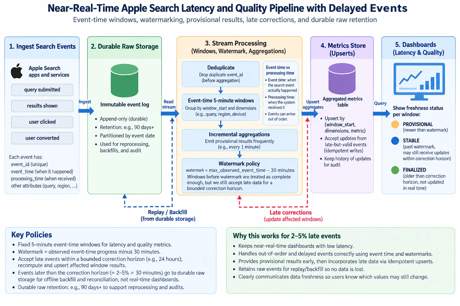
I would keep an immutable raw Search event log, deduplicate by event_id, and aggregate latency and quality into five-minute event-time windows. I would publish provisional results frequently, use a thirty-minute watermark to mark older windows as stable, and still allow bounded late corrections through idempotent upserts. After the correction horizon, values become finalized and very late events are handled through replay or backfill from raw storage. The trade-off is better completeness versus longer-lived mutable state and results.

Detailed Explanation

This question asks me to build a system that shows Apple Search speed and quality quickly even when some activity reports arrive much later than others. The difficult part is that an early number may not be the final number. I need to keep the original activity safely, avoid counting the same activity twice, update older totals when delayed information arrives, and clearly tell dashboard users which values may still change. I also need a clear point after which normal live processing stops changing old results.

Useful Questions to Ask the Interviewer
  1. Is a fixed five-minute reporting window appropriate for both latency and quality metrics?
  2. Should the watermark remain at thirty minutes, or may it be tuned from the measured lateness distribution?
  3. How long should late events remain eligible for real-time correction before requiring offline reconciliation?
  4. Is the diagram's example retention of 90 days or more sufficient for replay, backfill, and audit needs?
Design a near-real-time Apple Search latency and quality pipeline with delayed events. diagram
How to Explain It in an Interview
1. Ingest Search events with event and processing time

I would start with Apple Search app and service events such as query submitted, results shown, user clicked, and user converted. Each event carries a unique event_id, event_time, and processing_time, plus dimensions such as query, region, and device. event_time is when the action happened. processing_time is when the pipeline received it. This distinction matters because delayed events must still be assigned to the period in which the user action actually occurred.

2. Keep an immutable durable raw event log

Every event is appended to durable raw storage. The diagram shows an append-only event log partitioned by event date, with example retention of 90 days or more. This raw copy is the recovery source for reprocessing, backfills, and audits. I would not overwrite raw events during normal processing. If an aggregation must be rebuilt later, the pipeline can read the retained source events again instead of depending only on summarized data.

3. Deduplicate and build five-minute event-time windows

The processing path reads the stream and removes duplicate event_id values before aggregation. This prevents retries or repeated delivery from increasing metrics twice. Records are grouped into fixed five-minute event-time windows by window_start and the required dimensions. The pipeline calculates Search latency and quality metrics incrementally and emits provisional aggregates frequently, for example every minute, so the dashboard remains near real time.

4. Separate the watermark from the correction horizon

The watermark is max observed event_time - 30 minutes. It represents event-time progress and identifies older windows as complete enough to be considered stable. However, the diagram deliberately keeps a separate bounded correction horizon, such as 24 hours, because two to five percent of events arrive more than thirty minutes late. A late-but-valid event inside that correction horizon can still recompute its affected five-minute window. This gives fast results without pretending that the watermark means no later event can ever arrive.

5. Publish late corrections through idempotent upserts

Aggregates are stored using a logical key such as (window_start, dimensions, metric). Provisional writes and later corrections use upserts instead of blind inserts. That means repeating the same correction updates the existing logical result instead of creating another copy. When a valid delayed event changes an earlier window, the processor recomputes that window and upserts the corrected value. Keeping update history for audit helps explain why a published metric changed.

6. Show freshness directly on the dashboard

The dashboard exposes a status for every window. PROVISIONAL means the window is newer than the watermark and is expected to change. STABLE means it is past the watermark but still inside the correction horizon, so a delayed event may still update it. FINALIZED means it is older than the correction horizon and normal real-time processing no longer changes it. Events arriving after that point remain in durable raw storage and can be handled by replay, backfill, and reconciliation rather than silently changing finalized live values.

Technical Approach
  1. Append every Search event to the immutable durable raw event log with event_id, event_time, and processing_time.
  2. Read events into the processing path and remove duplicate event_id values before aggregation.
  3. Assign each event to a fixed five-minute window using event_time.
  4. Aggregate latency and quality metrics by window_start and the required dimensions.
  5. Emit provisional aggregate values frequently for near-real-time dashboards.
  6. Advance the watermark as observed event-time progress minus thirty minutes.
  7. Keep a separate bounded correction horizon, such as 24 hours, for late-but-valid events.
  8. Recompute affected windows when valid late events arrive and write corrections with idempotent upserts.
  9. Label dashboard windows as PROVISIONAL, STABLE, or FINALIZED based on the watermark and correction horizon.
  10. Reprocess retained raw events for replay, historical backfill, and reconciliation when data is outside the live correction horizon.
Practical Insights

The benefit is that dashboard users see Search latency and quality quickly without giving up the ability to correct delayed data. Five-minute windows keep the reporting grain understandable, while frequent provisional writes keep results fresh. The downside is that deduplication and window state must be kept while records may still arrive, and the aggregate store must support repeated idempotent updates. A longer correction horizon improves completeness but keeps results mutable for longer and increases state and operational cost. Durable raw retention also uses storage, especially when keeping 90 days or more. We accept these costs because raw retention makes replay and backfill possible, while a bounded correction horizon prevents old windows from remaining open forever.

Why Interviewers Ask This

This question tests whether a candidate can balance low-latency reporting with correctness when events arrive late or more than once. It evaluates judgment about event time, processing time, watermarks, deduplication, bounded correction windows, durable retention, idempotent publication, replay, and backfill. It also tests whether the candidate can communicate uncertainty clearly instead of presenting every near-real-time dashboard value as immediately final.

Common interview mistakes

Common mistakes are using processing time instead of event time, which assigns delayed events to the wrong reporting period; treating the thirty-minute watermark as a guarantee that no later events exist; dropping every event after the watermark even though the design has a longer correction horizon; failing to deduplicate repeated event_id values; inserting corrected aggregates as new rows instead of idempotently updating the existing logical aggregate; discarding raw events after aggregation; and showing dashboard values as final without distinguishing PROVISIONAL, STABLE, and FINALIZED states. Another mistake is allowing unlimited live corrections, which would keep old state open indefinitely.

Interview tip

Explain the design around one central idea: freshness and finality are different. Walk left to right from Search events, to immutable raw retention, deduplication, five-minute event-time windows, provisional aggregation, the thirty-minute watermark, bounded late corrections, idempotent upserts, and the three dashboard freshness states. Explicitly separate the watermark from the longer correction horizon.

Interviewer may ask next
What would you change if the percentage of events arriving more than thirty minutes late increased significantly?

I would first adjust the lateness policy rather than replace the architecture. The affected part is the event-time processing boundary between PROVISIONAL and STABLE results. If the observed delay distribution shows that thirty minutes is no longer enough, I would consider moving the watermark farther behind observed event-time progress. That would keep more delayed events in the normal event-time processing path and reduce the number of post-watermark corrections.

The correctness rules stay the same. I would still deduplicate by event_id, use five-minute event-time windows, retain the immutable raw log, and publish through idempotent upserts. I would also review the bounded correction horizon. If events are now commonly several hours late, that horizon may need to increase so those events can still correct affected windows without waiting for an offline backfill.

The downside is more retained processing state and a longer period before values become stable or finalized. I would base both thresholds on measured lateness instead of increasing them without evidence. Raw replay remains the recovery path beyond the live correction horizon.

How would you handle an event that arrives after its dashboard window has already been finalized?

I would keep it out of the normal real-time correction path and handle it through replay or backfill. In this design, FINALIZED means the window is older than the bounded correction horizon and normal live processing no longer changes it. The event is still retained because the immutable raw event log is the durable source for historical recovery.

I would reprocess the affected historical window from raw storage using the same event_id deduplication rule, the same five-minute event-time grain, and the same aggregate key. The recomputed result would be reconciled against the previously finalized value and written with the same idempotent upsert behavior so a repeated backfill does not create duplicate business results.

The requirement that changes is freshness: this is now an offline correction instead of a live update. The main downside is slower correction and extra reprocessing cost. The benefit is that the real-time pipeline remains bounded instead of keeping every historical window mutable forever.

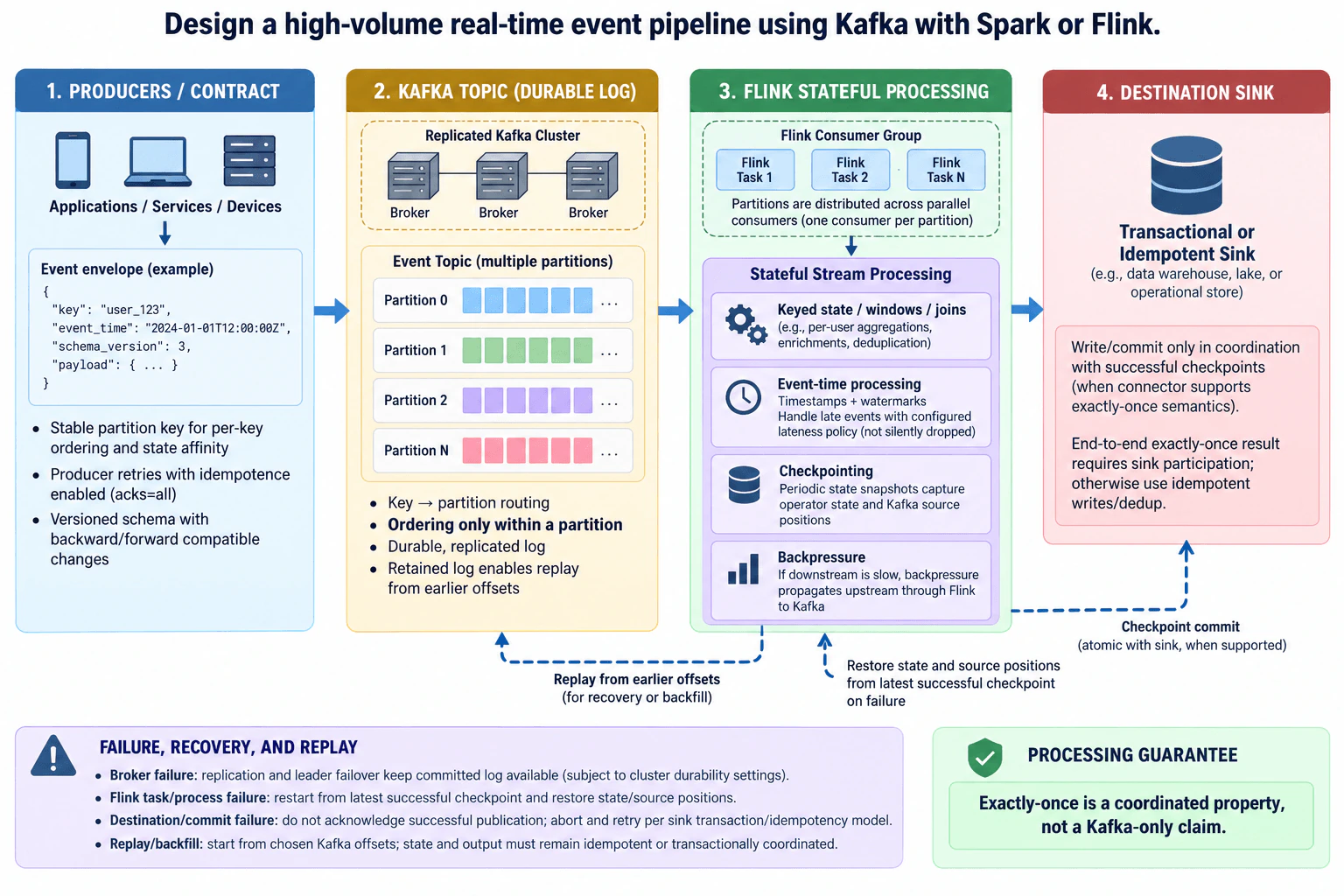
8. Design a high-volume real-time event pipeline using Kafka with Spark or Flink.Data PipelinesHardApple

Question Details

Specify producer contracts, topic and partition design, consumer groups, stateful transformations, event-time behavior, checkpointing, sink commits, backpressure, schema evolution, replay, and recovery from broker, processor, or destination failure while maintaining the stated processing guarantee.

Short Interview Answer (30-60 seconds)

I would use Kafka as the durable partitioned event log and Flink for stateful real-time processing. Producers use a versioned contract and stable partition key, while Flink handles event time, watermarks, checkpoints, and backpressure. For correctness, sink commits must coordinate with successful checkpoints when supported, or writes must be idempotent or deduplicated. More partitions improve parallelism, but they also increase coordination and operational overhead.

Detailed Explanation

This question asks me to design a system that can accept a very large number of events as they happen, keep them safely, process many of them at the same time, handle events that arrive late, and continue working when part of the system fails. I also need to explain how repeated work avoids repeated business results, how old events can be processed again, and how the system knows where to restart after a failure.

Useful Questions to Ask the Interviewer
  1. What end-to-end processing guarantee is required: at-least-once or exactly-once business results?
  2. What field should define per-key ordering and state affinity?
  3. How late can events arrive before they should no longer update results?
  4. Does the destination support transactional commits coordinated with processing checkpoints, or must writes be idempotent?
  5. How long must Kafka retain events for recovery, replay, and backfills?
Design a high-volume real-time event pipeline using Kafka with Spark or Flink. diagram
How to Explain It in an Interview
1. Define the producer contract

I would start by defining a stable event envelope. The diagram shows a key, event_time, schema_version, and payload. The stable key is used for Kafka partition routing, so related records keep per-key ordering and state affinity. Producers use retries with idempotence enabled and acks=all, which avoids duplicate Kafka records caused by producer retries when Kafka's idempotent producer guarantees apply. Schema changes are versioned and must follow the supported backward or forward compatibility policy instead of silently breaking existing consumers.

2. Use Kafka as the durable partitioned log

Producers send records to one Kafka event topic with multiple partitions. The key determines partition routing. Kafka provides ordering within a partition, not global ordering across the whole topic. Multiple partitions provide parallelism for high volume. The Kafka cluster is replicated, so a broker failure can be handled through replica and leader failover according to the cluster durability settings. Kafka retention is also the replay boundary. While the required records remain retained, processing can intentionally restart from earlier offsets for recovery or backfill.

3. Process partitions with a Flink consumer group

Flink reads Kafka as a consumer group and distributes topic partitions across parallel tasks. Within the group, one partition is assigned to only one consumer instance at a time, although one consumer may own multiple partitions. Flink then performs the stateful transformations shown in the diagram: keyed state, windows, joins, aggregations, enrichments, or deduplication. Keyed state keeps processing state aligned with the key. Useful parallelism is limited by Kafka partitioning, processing resources, state costs, and destination capacity.

4. Handle event time, checkpoints, and backpressure

The pipeline uses the producer's event_time to reason about when an event actually happened. Watermarks represent progress in event time and let stateful operators decide when event-time windows can advance. Late events are handled according to a configured lateness policy rather than being silently dropped. Flink periodically checkpoints operator state together with Kafka source positions. If a Flink task or process fails, it restarts from the latest successful checkpoint and restores both processing state and source progress. If downstream processing or the sink slows, Flink backpressure propagates upstream through the job toward the Kafka source instead of allowing unbounded work to accumulate inside the processor.

5. Coordinate destination commits with checkpoints

Processed records move to a transactional or idempotent destination sink. For an end-to-end exactly-once result, output visibility must be coordinated with successful Flink checkpoints when the connector and destination support that protocol. A failed or aborted processing attempt must not leave independently visible duplicate business results. If the sink cannot participate transactionally, writes must instead be idempotent or deduplicated, and I would describe the resulting guarantee accurately. Exactly-once is therefore a coordinated property of source progress, processor state, and destination commits, not a Kafka-only guarantee.

6. Recover, replay, and backfill safely

Broker failure is handled by Kafka replication and leader failover, subject to configured durability. A Flink processor failure restores the latest successful checkpoint and resumes from the source positions stored with that checkpoint. A destination or commit failure must not be acknowledged as successful publication; the write is aborted or retried according to the sink's transaction or idempotency model. Replay and backfill are different from normal checkpoint recovery because they intentionally begin from selected earlier Kafka offsets. During replay, state and output must still remain transactionally coordinated, idempotent, or deduplicated so processing the same input again does not create incorrect repeated results.

Technical Approach
  1. Define the producer event envelope with a stable partition key, event time, schema version, and payload.
  2. Produce records to a replicated Kafka topic using the key for partition routing and per-key ordering.
  3. Use a Flink consumer group to distribute partitions across parallel tasks.
  4. Apply keyed stateful transformations using event time and watermarks.
  5. Periodically checkpoint operator state and Kafka source positions.
  6. Let Flink backpressure slow upstream consumption when downstream processing or the sink is constrained.
  7. Commit output transactionally with successful checkpoints when supported; otherwise use idempotent destination writes or deduplication.
  8. Recover processor failures from the latest successful checkpoint and use retained Kafka offsets for intentional replay or backfill.
Practical Insights

The benefit is that Kafka partitions let the pipeline spread work across many Flink tasks, while retained events and checkpoints make recovery practical. The downside is that adding partitions is not free: it creates more broker, consumer, state, and coordination work. Event-time processing gives more correct results when events arrive out of order, but waiting for late events can delay final results. Checkpoints reduce recovery work, but frequent checkpoints add storage and processing overhead. Longer Kafka retention gives more replay and backfill flexibility, but uses more storage. Transactional sink commits give stronger correctness when supported, but they require connector and destination participation. We accept these costs because the design prioritizes high throughput, recoverability, and controlled duplicate behavior.

Why Interviewers Ask This

Interviewers ask this to test whether you can reason about a streaming system as one end-to-end correctness problem rather than a list of technologies. They want to see whether you understand data contracts, partitioning and ordering, stateful event-time processing, checkpoints, backpressure, replay, and failure recovery. The key judgment is recognizing that Kafka durability and Flink checkpoints alone do not guarantee exactly-once business results; the destination commit behavior must participate in the design.

Common interview mistakes

Common mistakes are claiming Kafka provides global ordering instead of ordering only within a partition; choosing a changing or poorly distributed partition key; claiming exactly-once because Kafka or Flink supports it without checking destination commit behavior; advancing source progress before output is safely committed; ignoring late events and watermark behavior; assuming checkpoints remove the need for Kafka retention; retrying destination writes without transactional coordination, idempotency, or deduplication; treating checkpoint recovery as the same thing as a historical backfill; and scaling Flink workers without checking whether Kafka partition count or destination capacity is the real bottleneck.

Interview tip

Explain the design from left to right: producer contract, Kafka partitioning, Flink state and event time, checkpoints and backpressure, then destination commits. Spend extra time on failure boundaries. Clearly state that ordering is per partition and that exactly-once business results require coordination across source progress, processor state, and destination writes.

Interviewer may ask next
What would you change if the destination became much slower and the Kafka consumer lag kept increasing?

I would keep the same Kafka-to-Flink-to-sink architecture and first treat the destination as the limiting resource. Flink backpressure should propagate from the slow sink through the processing graph toward the Kafka source, preventing the processor from accepting unlimited in-memory work. I would check whether the destination can safely handle more parallel writes before increasing Flink parallelism. If it can, I can increase useful processing parallelism up to the limits imposed by Kafka partitions, Flink state, and sink capacity. If the destination cannot scale, adding consumers only moves the bottleneck and can increase state and coordination overhead. Correctness does not change: checkpoints must still capture consistent processor state and Kafka source positions, and destination commits must remain checkpoint-coordinated when supported or idempotent or deduplicated otherwise. Kafka retention must be long enough to hold the growing backlog until the sink recovers. The main downside is higher end-to-end latency and potentially higher storage and recovery cost while lag accumulates.

How would you safely replay several hours of Kafka events after discovering that the earlier processing result was wrong?

I would perform an intentional replay from selected Kafka offsets rather than treating it as an ordinary checkpoint restart. The requirement changes because we deliberately want to process historical input again, while normal failure recovery resumes from the latest successful checkpoint. Kafka retention provides the source records needed for that replay. I would choose offsets covering the affected period and make sure the Flink state used for the replay is consistent with that replay boundary. The destination remains the critical correctness point: replayed records must not create accidental duplicate business results, so output still needs transactional coordination when supported or an idempotent or deduplicating write model. I would keep the same producer contract, partitioning, event-time logic, watermarks, and stateful transformations. Recovery is verified by confirming that processing reaches the intended Kafka positions and that destination commits complete under the same correctness rule. The main downside is extra compute, state work, Kafka read traffic, and destination write load while historical data is processed again.

9. Explain how Parquet reduces cloud query work.Cloud Data PlatformsEasyApple

Question Details

Relate column projection, row-group statistics, predicate pushdown, typed encoding, compression, and partition pruning to bytes read and compute consumed for a concrete analytical query. Include a case where poor file size, sort order, or high-cardinality partitioning prevents those benefits.

Short Interview Answer (30-60 seconds)

Parquet reduces cloud query work by pruning irrelevant partitions and row groups, reading only required columns, and using typed encodings plus compression. That means fewer bytes are read, decompressed, decoded, and aggregated, although tiny files, poor sort order, or excessive partitioning can weaken the savings.

Detailed Explanation

For repeated cloud analytics, the practical problem is avoiding unnecessary storage reads and compute on every query. Parquet helps because its physical layout gives the query engine several chances to eliminate data before aggregation. In this design, the reusable data-platform capability is a partitioned Parquet dataset that query workloads can scan efficiently. The example query needs customer_id and amount for one sale date and one region, with amount greater than 100. The design prioritizes reducing the files, columns, row groups, and compressed bytes that must be read and processed.

Useful Questions to Ask the Interviewer
  1. Which columns are most commonly used as partition filters and row predicates?
  2. How are the Parquet datasets currently partitioned, and do common queries include those partition columns?
  3. Are the files large enough to avoid excessive planning and file-open overhead?
  4. Is data sorted or clustered on frequently filtered columns so row-group statistics remain selective?
  5. Are any high-cardinality partition keys creating too many small partitions or files?
Explain how Parquet reduces cloud query work. diagram
How to Explain It in an Interview
  1. Start with the concrete analytical query The query selects customer_id and SUM(amount) from sales where sale_date is DATE '2026-09-01', region is 'US', and amount is greater than 100, then groups by customer_id. The goal is to avoid scanning the complete sales dataset. The normal flow is query to partition pruning, then Parquet column scanning and predicate evaluation, then row-group skipping, decompression and decoding, and finally aggregation in the query engine.
  1. Prune partitions before reading unrelated files The sales dataset is partitioned by sale_date and region. Because the query specifies sale_date=2026-09-01 and region=US, the engine can select that matching partition and avoid the other dates and regions shown in the diagram. Those unrelated partition files are not read. This immediately reduces the number of files and storage bytes considered by the scan. The trade-off is that partitioning works best when the keys match common filters without creating an excessive number of partitions.
  1. Project only the columns the query needs Parquet is columnar, so the engine does not need to read every column in each selected file. For this query, customer_id and amount are the needed data columns. The sale_date and region filters are already resolved through the selected partition path in this design. Other Parquet columns can remain unread. Reading fewer column chunks means fewer bytes are fetched and less data must later be decompressed and decoded.
  1. Push the amount predicate into the Parquet scan The predicate amount > 100 is pushed down to the Parquet scan instead of waiting until all candidate file data has been fully processed by the query engine. Predicate pushdown lets the scan layer use available Parquet metadata to eliminate data early. It does not mean that every failing row can always be rejected from metadata alone; rather, it creates the opportunity to skip larger physical regions such as row groups when their statistics prove they cannot match.

5. Use row-group statistics to skip impossible matches The diagram shows min/max statistics for amount at row-group level. Row Group 1 has amount values from 0 to 50, and Row Group 2 from 51 to 99. Neither group can satisfy amount > 100, so both can be skipped. Row Group 3 spans 101 to 500 and Row Group 4 spans 200 to 1000, so those groups may contain matching rows and must be read. Skipping whole row groups reduces bytes scanned before row-level filtering and aggregation.

  1. Use typed encoding and compression to reduce physical I/O Parquet stores typed columns such as long, decimal, date, and string and can use encodings suited to the data, including dictionary and run-length encoding where appropriate. The encoded column pages are then compressed, for example with Snappy as shown in the diagram. Encoding can make the representation more compact and can improve compression effectiveness. Compression reduces the physical bytes stored and transferred. After pruning and projection, the engine decompresses and decodes only the remaining selected column data.
  1. Aggregate the smaller surviving data set After partition pruning, column projection, predicate pushdown, and row-group skipping, the query engine performs GROUP BY customer_id and SUM(amount) on a much smaller input. The diagram summarizes the consequence as fewer partitions, files, columns, and row groups read; less data to decompress and decode; fewer bytes read from storage; and therefore less CPU and memory consumed before producing customer_id and total_amount.
  1. Explain when the benefits are reduced Parquet does not automatically guarantee an efficient scan. Too many tiny files increase planning, metadata, and file-open overhead. Poor sort order on amount can make row-group minimum and maximum ranges overlap widely, so fewer groups can be skipped. Overly granular or high-cardinality partitioning can create many small partitions and files, increasing metadata work and reducing the practical benefit of partition pruning. In those cases, the same query reads more data and consumes more compute than it would with a well-organized layout.
Technical Approach
  1. Start from a representative analytical query and identify its partition filters, row predicates, projected columns, and aggregation keys.
  2. Use partition predicates such as sale_date and region to eliminate unrelated files.
  3. Project only the Parquet columns needed by the query.
  4. Push row predicates such as amount > 100 into the Parquet scan.
  5. Use row-group min/max statistics to skip groups that cannot satisfy the predicate.
  6. Read, decompress, and decode only the selected column chunks from the surviving row groups.
  7. Aggregate the reduced input in the query engine.
  8. Review file size, sort order, and partition cardinality because poor physical layout can prevent these reductions.
Practical Insights

The query cost depends mainly on how much data survives each pruning step rather than only on the table's total logical size. Partition pruning reduces files read. Column projection reduces column bytes read. Row-group statistics can remove additional data inside selected files. Compression reduces physical storage I/O, while typed encoding can make values more compact and easier to encode efficiently. The surviving data still costs CPU and memory to decompress, decode, filter, group, and aggregate. Tiny files add planning and open overhead. Poor sort order can make row-group statistics ineffective. Very high-cardinality partitioning can create too many partitions, files, and metadata operations.

Why Interviewers Ask This

Interviewers want to see whether the candidate can connect Parquet's physical layout to actual cloud query work. A strong answer explains exactly how partition pruning, column projection, predicate pushdown, row-group statistics, typed encoding, and compression reduce bytes read and compute, and why poor file layout can prevent those optimizations.

Common interview mistakes

Common mistakes are saying only that Parquet is columnar without connecting that fact to bytes read; confusing partition pruning with row-group skipping; claiming predicate pushdown means every non-matching row is eliminated without reading data; forgetting that row-group statistics can skip a group only when they prove the predicate cannot match; assuming compression removes CPU work even though data must still be decompressed; assuming Parquet guarantees good pruning regardless of sort order; creating too many tiny files; and partitioning on very high-cardinality keys that create excessive metadata and file overhead.

Interview tip

Use one concrete query and trace what disappears at each stage: unrelated partitions, unused columns, impossible row groups, and then non-matching rows. Connect each reduction to fewer bytes read and less decompression, decoding, CPU, and memory. Finish with tiny files, poor sort order, and high-cardinality partitioning as the main failure cases.

Interviewer may ask next
What happens if the Parquet files are not sorted on the column used by the amount > 100 filter?

Partition pruning and column projection can still work, but row-group skipping may become much less effective. If amount values are widely mixed inside every row group, each group's minimum and maximum range may span both values below and above 100. Because each group could still contain a match, the engine cannot safely skip it from statistics alone. It must read, decompress, and decode more selected column data before applying the row-level filter. Better sort or clustering order on a frequently filtered column can produce narrower row-group ranges and make min/max statistics more selective.

Why can high-cardinality partitioning make Parquet queries worse even though partition pruning is useful?

Partition pruning is most useful when a partition key creates a manageable number of meaningful groups that match common query filters. A high-cardinality key can instead create a very large number of tiny partitions and files. The query engine then has more metadata to inspect, more files to open, and less useful data in each file. That planning and file-open overhead can offset pruning gains. In this design, bounded filters such as sale_date and region are better partition candidates, while more selective predicates such as amount can rely on Parquet's internal organization and row-group statistics.

10. Design a platform for iCloud storage dashboards and weekly analytics.Cloud Data PlatformsMediumApple

Question Details

Select ingestion, object storage, table format, transformation compute, low-latency serving, and historical query components. Explain how the platform supports fresh per-account-safe usage, weekly trends, backfills, access controls, lifecycle tiers, and cost isolation between operational dashboards and exploratory scans.

Short Interview Answer (30-60 seconds)

I would separate fresh dashboard serving from historical analytics: Kafka and Flink produce per-account aggregates, Iceberg on object storage keeps durable history, ClickHouse serves low-latency dashboards, and Trino handles exploratory scans. The main trade-off is extra platform complexity in exchange for workload and cost isolation.

Detailed Explanation

iCloud dashboards need fresh usage by account, while analysts also need weekly trends and large historical scans. Those workloads have different latency and cost characteristics, so one query system should not serve both. I would build a reusable platform where iCloud services publish account-keyed usage events, Flink creates fresh aggregates, Iceberg keeps the durable analytical record, ClickHouse serves operational dashboards, and Trino reads history. A separate control plane owns identity, metadata, policy, quotas, cost attribution, audit, and observability so governance stays separate from the production record path.

Useful Questions to Ask the Interviewer
  1. What freshness target do the per-account iCloud dashboards require?
  2. How much historical data must remain in hot, cool, and archive storage tiers?
  3. What isolation level is required between accounts beyond the shown per-account authorization and row-level controls?
  4. How much concurrency should operational dashboard traffic and analyst exploration support independently?
  5. What recovery expectations exist if ingestion, transformation, serving, or catalog components are temporarily unavailable?
Design a platform for iCloud storage dashboards and weekly analytics. diagram
How to Explain It in an Interview
1. Start with the two workload classes

The platform has two main consumer patterns. iCloud dashboards need fresh, low-latency per-account usage. Data analysts need weekly trends, deep analysis, and ad-hoc historical queries. I would deliberately isolate these workloads because an exploratory scan should not consume the same serving capacity used by operational dashboards.

The input is iCloud storage usage activity from services such as photos, files, and backups. Events include account_id as the isolation key, plus usage-related attributes and timestamps. The platform must preserve that account boundary through processing and serving.

2. Define users and ownership

Producer-side iCloud services own the correctness of the usage events they emit. The shared platform owns Kafka ingestion, Flink processing, object storage and Iceberg tables, ClickHouse serving, Trino historical querying, scheduling, metadata, access policy, quotas, cost attribution, audit, and observability.

The consumers are iCloud dashboards and data analysts. Dashboards query ClickHouse for per-account usage. Analysts query Iceberg through Trino for weekly trends, deep historical analysis, and ad-hoc exploration.

The diagram does not name a portal, CLI, or API for self-service provisioning, so I would not invent one. The reusable platform boundary is the shared ingestion, processing, storage, serving, catalog, scheduling, policy, and observability foundation. Teams reuse those capabilities instead of building separate foundations for each workload.

3. Keep the control plane separate from production data

The control plane contains four concerns. Identity and Access Management holds per-account policies and row-level access controls. Data Catalog and Metadata holds the Iceberg catalog, lineage, and schema-evolution metadata. Policy, Quotas, and Cost Attribution separates dashboard and exploratory resource usage. Audit and Observability records access, usage, and cost signals.

The dashed arrows represent control flows such as policies, metadata, and quotas. They do not carry iCloud usage records. Production records remain in the data plane, where Kafka, Flink, object storage, ClickHouse, and Trino process or query them.

This separation keeps policy and metadata responsibilities distinct from record processing. The diagram does not define a manual approval process, so I would not claim one.

4. Ingest account-keyed usage through Kafka

The normal data path starts when iCloud services emit storage usage events into Kafka. Kafka is the reusable ingestion layer for the streaming workload. The event contract carries account_id as the isolation key together with usage data and timestamps needed for downstream aggregation.

The diagram explicitly calls out idempotent producers. That reduces duplicate publication caused by producer retries, but it does not prove exactly-once business results across Flink, Iceberg, and ClickHouse. Downstream processing still needs deterministic keys and idempotent or reconcilable output behavior.

If ingestion or processing falls behind, Kafka consumer lag is an important signal. Records that are still available within Kafka retention can be replayed after recovery.

5. Use Flink for fresh aggregates and historical recomputation

Kafka sends events to Apache Flink. Flink owns stream processing for fresh per-account aggregates. Those aggregates flow to ClickHouse for near-real-time dashboard serving.

Flink also performs batch and backfill recomputation from Iceberg. A scheduler or orchestrator triggers weekly aggregation jobs, backfills, and data-quality checks. The scheduler coordinates when work runs; Flink performs the transformation itself.

For a failed streaming task, I would monitor lag and processing health, restore processing, and validate the resulting aggregates. For a historical correction, I would read the affected Iceberg history and run a bounded recomputation. Restarting a task is a retry; rebuilding derived results from Iceberg is a backfill or recomputation.

6. Keep the durable analytical record in object storage with Iceberg

Flink writes canonical usage records to durable object storage organized as Apache Iceberg tables. Iceberg provides the table layer over the physical objects. The design uses snapshots, schema evolution, partitioning, and ACID table semantics for the historical analytical record.

The canonical records retain account_id so downstream jobs and queries can preserve the account boundary. The catalog stores table and schema metadata rather than production usage records.

The object-storage layer has hot recent, cool older, and long-term archive lifecycle tiers. Moving older data to cheaper tiers reduces storage cost, but archived data can require different retrieval behavior before it is practical to query or backfill. Lifecycle policy therefore has to match the required analytical and recovery access pattern.

7. Serve operational dashboards from ClickHouse

Fresh per-account aggregates flow from Flink into ClickHouse. ClickHouse is the dedicated low-latency serving store for operational dashboard queries. iCloud dashboards query this serving layer instead of scanning Iceberg history directly.

The serving model must preserve account_id and apply the per-account access policy shown in the control plane so a dashboard request only reads data allowed for that account context.

This creates derived state outside the durable Iceberg history, so there is a freshness and consistency trade-off. If ClickHouse falls behind or must be rebuilt, the platform can recompute aggregates from Iceberg through Flink and republish them to ClickHouse.

8. Use Trino for weekly trends and historical exploration

Trino queries Iceberg tables for historical analytics. Data analysts use this path for weekly trends, deep analysis, and ad-hoc queries. It is deliberately separate from the ClickHouse dashboard-serving path.

The diagram assigns exploratory analytics a separate compute pool and quotas. That prevents large historical scans from competing directly with the operational serving capacity. Cost attribution also keeps exploratory scans distinguishable from dashboard-serving costs.

This separation increases the number of systems to operate, but it lets each engine match its access pattern and creates clearer performance and cost boundaries.

9. Enforce access, metadata, lifecycle, and cost controls centrally

Identity and access policies define who may access per-account data. The catalog records Iceberg metadata, lineage, and schema evolution. Quotas and workload-specific compute boundaries isolate dashboard serving from analyst exploration. Audit and observability collect evidence about access, usage, and cost.

These controls must be enforced at the relevant processing, storage, serving, and query boundaries. A catalog entry describes metadata; it does not itself authorize a user. Likewise, account_id is an isolation key, not a complete isolation mechanism unless authorization rules are applied to it.

10. Observe each workload at its own boundary

For Kafka and Flink, I would watch ingestion health, consumer lag, processing failures, and job state. For scheduled weekly work and backfills, I would monitor run status and the shown data-quality checks. For ClickHouse, the main consumer-facing signals are serving freshness and query behavior. For Trino, I would watch exploratory query activity and resource consumption. The control plane also records access, usage, and cost evidence.

The first bottleneck depends on the real workload, which the question does not quantify. It could appear in ingestion, Flink processing, ClickHouse serving concurrency, Iceberg table maintenance, or Trino query capacity. I would find it from those workload-specific signals instead of inventing throughput numbers.

11. Recover using the durable boundaries

Kafka can support replay for records still inside its configured retention window. Iceberg on object storage is the durable historical basis for recomputation and backfills. The scheduler triggers bounded recovery work, while Flink rebuilds the affected aggregates.

If ClickHouse derived data becomes stale or incorrect, the platform can recompute it from Iceberg through Flink and republish the result. After recovery, the shown data-quality checks should validate the rebuilt data before it is treated as correct again.

The diagram does not specify multi-region failover, replication topology, recovery-time objectives, or recovery-point objectives, so I would not claim them.

12. Handle schema and platform evolution carefully

Iceberg schema evolution and the shared metadata catalog provide a controlled way to evolve historical tables. Producer event contracts still need compatibility rules so a schema change does not silently break Flink processing, ClickHouse serving, or Trino queries.

For historical corrections, the scheduler triggers a backfill and Flink recomputes from Iceberg. The rebuilt serving aggregates can then be republished to ClickHouse. This keeps correction work separate from the normal streaming path.

The diagram does not define an existing-system migration or a dual-run cutover, so I would not invent one. New workloads should adopt the shared ingestion, storage, policy, serving, and analytics capabilities instead of creating parallel foundations.

13. Summarize the main trade-offs

The design accepts more operational complexity to isolate unlike workloads. Kafka and Flink add streaming infrastructure so dashboards can stay fresh. Iceberg on object storage provides durable, replayable analytical history but is not the low-latency dashboard store. ClickHouse gives fast serving but holds derived state that must stay consistent enough with the durable history. Trino gives analysts flexible SQL over Iceberg but receives separate compute and quotas so exploratory scans cannot dominate operational workloads.

The final platform therefore prioritizes fresh per-account-safe usage, weekly trends, backfills, enforceable access controls, lifecycle tiers, and explicit cost isolation between dashboard serving and exploratory scans.

Technical Approach
  1. Separate the two consumer workloads: low-latency per-account dashboards and historical analyst queries.
  2. Define account_id as the isolation key carried by iCloud usage events.
  3. Ingest usage events through Kafka and use idempotent producer behavior without claiming end-to-end exactly-once results.
  4. Process fresh per-account aggregates with Flink and send those aggregates to ClickHouse.
  5. Write canonical usage records to object storage organized as Apache Iceberg tables.
  6. Use the scheduler or orchestrator to trigger weekly aggregation jobs, data-quality checks, and historical backfills executed by Flink.
  7. Serve operational dashboards from ClickHouse and historical or exploratory SQL from Trino over Iceberg.
  8. Apply identity, row-level access policy, catalog metadata, lineage, quotas, cost attribution, audit, and observability through the separate control plane.
  9. Move historical objects through hot, cool, and archive lifecycle tiers according to retention and access needs.
  10. Isolate dashboard serving and exploratory scans with separate compute capacity and quotas, then attribute their costs separately.
  11. Recover by replaying Kafka records that remain within retention or by recomputing derived data from Iceberg, followed by data-quality validation.
Practical Insights

The design scales each workload independently instead of assuming one system must absorb all growth. Kafka and Flink scale with incoming event and processing pressure. Object storage grows with retained history, while Iceberg metadata and table maintenance also need attention as files, partitions, and snapshots accumulate. ClickHouse capacity follows dashboard freshness and query-concurrency needs. Trino capacity follows analyst concurrency and the amount of historical data scanned. Separating ClickHouse from Trino prevents large exploratory scans from directly competing with operational dashboard queries, but it increases operational complexity. Lifecycle tiers reduce the cost of retaining older objects, with the trade-off that archived data can be slower or less convenient to access for analysis and backfills. Compute, network, and storage costs also increase when data is transformed, republished, or scanned repeatedly. No exact throughput, latency, storage size, or cost number is assumed because the question does not provide one.

Why Interviewers Ask This

This question tests whether a Data Engineer can design a reusable platform around different access patterns instead of forcing every workload through one storage or compute engine. A strong answer separates operational dashboard serving from historical exploration, preserves the per-account security boundary, distinguishes the control plane from production data movement, supports replay and backfills, and explains lifecycle and compute isolation as cost controls.

Common interview mistakes

Common mistakes are using the Iceberg lake directly for every dashboard query, which mixes historical scans with a low-latency serving requirement; using ClickHouse as the only durable history source; forgetting account_id and the per-account authorization boundary; claiming Kafka producer idempotence makes the whole platform exactly once; saying the scheduler performs transformations instead of Flink; treating the catalog as if it stores production records; putting production records through the control plane; running Trino exploration in the same capacity pool as operational serving; forgetting weekly backfills and recomputation from Iceberg; calling a simple task restart a completed recovery; assuming archived data has the same access behavior as hot data; and inventing multi-region guarantees, service levels, volumes, or latency targets that are not given.

Interview tip

Lead with the workload split. Explain that fresh per-account dashboards and historical exploration have different latency and cost needs, then trace one normal event from iCloud through Kafka and Flink to durable Iceberg history and ClickHouse serving. Finish with backfills, access enforcement, lifecycle tiers, and why Trino gets isolated exploratory capacity.

Interviewer may ask next
What would you do if a bug in a Flink transformation produced incorrect per-account dashboard aggregates for several days?

I would first correct or stop the faulty Flink logic so new events no longer produce bad aggregates. Then I would use the scheduler or orchestrator to start a bounded backfill over the affected Iceberg history. Flink would recompute the per-account aggregates with the corrected logic and republish the derived results to ClickHouse. The shown data-quality checks would validate the rebuilt output before recovery is considered complete. Observability should identify the affected freshness or correctness window so dashboard consumers are not silently shown data that is known to be under correction. This is recomputation from durable history, not merely a retry of the failed task.

How would you stop a large analyst query from hurting iCloud dashboard performance as historical usage grows?

I would keep the architecture's workload-isolation boundary. Dashboards continue to query ClickHouse, while analysts query Iceberg through Trino. Trino uses the separate exploratory compute pool and quotas shown in the design, so a large historical scan does not consume the serving capacity used by ClickHouse. The control plane attributes usage and cost separately for dashboard serving and exploratory scans. Older Iceberg data can also move through hot, cool, and archive lifecycle tiers according to retention and access needs. The trade-off is additional platform complexity, but it protects the operational serving path and makes exploratory cost visible.

More questions load as you scroll

Disclaimer: This interview guide is for educational and informational purposes only. It is designed to help readers prepare, but it does not guarantee any interview result, hiring decision, offer, or outcome. Interview questions, hiring criteria, and preferred answers can vary by employer, interviewer, industry, location, and time. The examples and explanations reflect the authors' research and judgment, are provided without warranties of any kind, and should not be treated as the only correct approach. Diagrams are simplified illustrations intended to highlight the main components and their interactions; actual systems and implementations may be more complex. Alternative approaches may be equally valid or better suited to a particular question, context, or interviewer. To the fullest extent permitted by applicable law, the author, contributors, and publisher are not liable for decisions made, actions taken, or losses incurred based on this guide.

Company Notice: This guide is an independent educational resource and is not affiliated with, endorsed by, sponsored by, or approved by the company named in this guide. Company names are used only to identify interview experiences commonly reported by candidates. Interview practices can change without notice, and inclusion of company-specific content does not mean these questions are official, complete, or guaranteed to be asked. To the fullest extent permitted by law, the author, contributors, and publisher are not responsible for outcomes related to use of this material.

Content Accuracy and Verification: To the fullest extent permitted by applicable law, we do not represent or warrant that interview guides, questions, answers, examples, or diagrams are accurate, complete, current, error-free, or suitable for any particular purpose. You are responsible for independently reviewing and verifying the information before relying on it.