15 Google Data Engineer Interview Questions & Answers

google icon

Questions with Detailed ExplanationsWith Detailed Explanations

(Last Updated: September 8, 2026)

1. Design a schema to track user interactions with local ads over time.Data ModelingEasyGoogle

Question Details

Declare separate grains for ad impressions, clicks, calls, direction requests, and attributed outcomes. Include stable identifiers for campaign, creative, placement, region, device class, privacy-safe user or session, and event time; preserve repeated legitimate interactions while making client retries detectable. Explain the relationships needed for regional performance reporting without joining facts at mixed grains.

Short Interview Answer (30-60 seconds)

I would use separate event-grain fact tables for impressions, clicks, calls, direction requests, and outcomes, all linked many-to-one to one conformed ad-context dimension. Each event has its own event ID and client retry ID. For reporting, aggregate facts separately to one common grain before combining them.

Detailed Explanation

The main decision is to store each kind of ad activity separately because an ad being shown is not the same event as a click, phone call, direction request, or later business result. Every real interaction should stay as its own record, even when the same person repeats an action. At the same time, accidental resends from a client should be recognizable. Shared information such as campaign, creative, placement, region, and device type should use one consistent definition so regional reports can compare the different activities without accidentally multiplying records or counting the same activity more than intended.

Useful Questions to Ask the Interviewer
  1. What should count as an attributed outcome: a purchase, store visit, lead, or several outcome types?
  2. What time zone should define the reporting date for regional reports?
  3. How long should client_event_id values remain available for retry detection?
  4. Can anonymous_user_key or session_id be missing when privacy or collection rules prevent identifying a user or session?
  5. Is attribution limited to a triggering click, as shown in the supplied model, or may future attribution need to reference other interaction types?
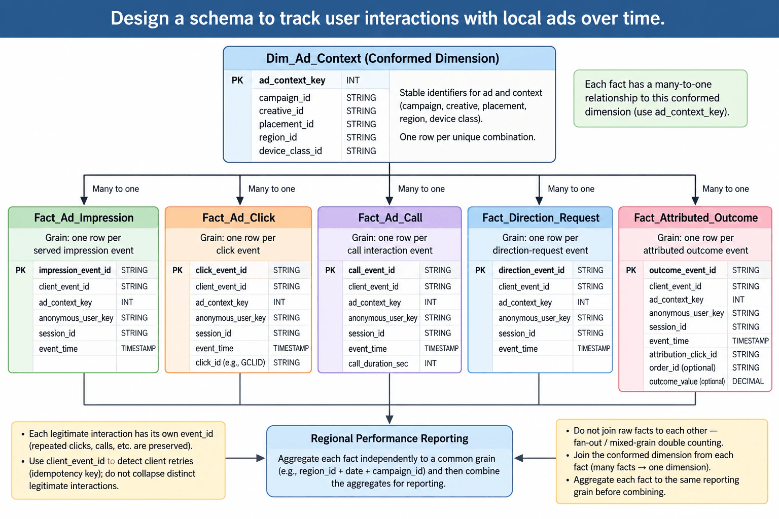
Design a schema to track user interactions with local ads over time. diagram
How to Explain It in an Interview

I would start by declaring the grain of every fact table. Grain means exactly what one row represents.

  • Fact_Ad_Impression: one row per served impression event.
  • Fact_Ad_Click: one row per click event.
  • Fact_Ad_Call: one row per call interaction event.
  • Fact_Direction_Request: one row per direction-request event.
  • Fact_Attributed_Outcome: one row per attributed outcome event.

Each fact has its own event-level primary key: impression_event_id, click_event_id, call_event_id, direction_event_id, or outcome_event_id. This preserves legitimate repeated behavior. If the same user clicks twice, those are two distinct click events rather than one row being overwritten or removed as a duplicate.

Each fact also stores client_event_id. In this model, client_event_id is the retry-detection or idempotency identifier for a client submission. If the same submission is retried, the repeated delivery can be recognized using that identifier. A legitimate second interaction has its own event identity and should not be collapsed merely because the user, campaign, region, or timestamp looks similar.

The shared Dim_Ad_Context table is a conformed dimension. Conformed means the same dimension definition is reused consistently across multiple fact tables. It has the surrogate primary key ad_context_key and stable identifiers for campaign_id, creative_id, placement_id, region_id, and device_class_id. One dimension row represents one unique combination of those ad-context identifiers.

Every fact contains ad_context_key and has a many-to-one relationship to Dim_Ad_Context: many event rows can point to one ad-context row. Each fact also stores event_time and the privacy-safe identifiers anonymous_user_key and session_id shown in the diagram.

The event-specific columns remain only in the facts where they make sense. Fact_Ad_Click contains click_id, such as a GCLID when that identifier is available. Fact_Ad_Call contains call_duration_sec. Fact_Attributed_Outcome contains attribution_click_id and can contain optional order_id and optional outcome_value.

For regional performance reporting, I would not join the raw fact tables directly to each other. They have different grains and different numbers of rows. Joining them through common values such as region or campaign can create fan-out, where one fact row matches several rows from another fact and inflates counts or values.

Instead, I would join each fact independently many-to-one to Dim_Ad_Context and aggregate each fact to the same reporting grain. The diagram uses region_id + date + campaign_id as an example. I would produce separate impression, click, call, direction-request, and outcome aggregates at exactly that grain. Only then would I combine those same-grain aggregate results for reporting.

This design uses more fact tables than a single generic event table, but it makes the business meaning and grain of every row explicit. It also keeps event-specific fields in the correct place and reduces the risk of mixed-grain reporting errors. The operational tradeoff is that ingestion must maintain reliable event IDs, client_event_id retry detection, and consistent ad_context_key lookups. This is a conceptual data-modeling design, so no database-specific SQL dialect or engine behavior is required.

Technical Approach
  1. Identify the five business processes: impression, click, call, direction request, and attributed outcome.
  2. Declare one event-level grain for each corresponding fact table.
  3. Give every legitimate interaction its own immutable event primary key.
  4. Store client_event_id separately so retries of one client submission are detectable without collapsing genuine repeated interactions.
  5. Store event_time plus the privacy-safe anonymous_user_key and session_id shown in the model.
  6. Create Dim_Ad_Context with ad_context_key and stable campaign, creative, placement, region, and device-class identifiers.
  7. Link every fact many-to-one to Dim_Ad_Context using ad_context_key.
  8. Keep event-specific attributes only on their appropriate facts, such as call_duration_sec or outcome_value.
  9. For regional reporting, aggregate each fact independently to the same grain, such as region_id + date + campaign_id.
  10. Combine only those same-grain aggregates instead of joining raw facts together.
Practical Insights

Storage grows with the number of legitimate interaction events because impressions, clicks, calls, direction requests, and outcomes are all retained separately. Retry detection adds ingestion work because client_event_id values must be checked or tracked. Regional reporting must scan and aggregate each relevant fact independently before combining results, so query cost depends on the event volume being analyzed. The model has more tables than a single mixed event table, but maintenance is safer because every fact has one clear grain and event-specific columns stay in the correct table.

Why Interviewers Ask This

This question tests whether the candidate can define precise fact-table grains, model shared dimensions, preserve legitimate repeated events, support retry detection, and avoid fan-out and double counting when different interaction facts are combined for regional analytics.

Common interview mistakes

A common mistake is storing impressions, clicks, calls, direction requests, and outcomes in one table without a precise row grain. Another is treating repeated interactions from the same user as duplicates and deleting legitimate second or third events. Using no separate retry identifier makes client resends harder to distinguish from real activity. The most serious reporting mistake is joining raw fact tables together on region, campaign, user, or session, which can create fan-out and inflate counts. Other mistakes include duplicating shared ad-context attributes inconsistently across facts, putting event-specific measures in the dimension, or combining aggregates before every source has been reduced to the same reporting grain.

Interview tip

State the five fact grains first. Then explain the two main correctness rules: client_event_id detects retries without removing legitimate repeated events, and raw facts are not joined at mixed grains. Finish by showing that every fact links many-to-one to the same conformed ad-context dimension and is aggregated independently before regional metrics are combined.
Interviewer may ask next
How would you detect a client retry without removing two legitimate clicks from the same user?

Keep the event identity and the retry-detection identity separate. Every legitimate click has its own click_event_id. client_event_id identifies the client submission so a retry of that same submission can be recognized. A genuine second click receives its own event identity and should remain a separate fact row. I would not deduplicate only by user, campaign, region, or timestamp because different real interactions can legitimately share those values.

Why not join impressions, clicks, calls, and outcomes directly on region_id and campaign_id?

Those fact tables have different event grains and different row counts. A region and campaign can contain many impressions, many clicks, many calls, and many outcomes. Joining the raw facts on shared dimension values can multiply matching rows and inflate counts or monetary values. Instead, aggregate each fact independently to the same grain, such as region_id + date + campaign_id, and then combine the resulting one-row-per-grain aggregates.

2. Model YouTube watch events for daily watch-time reporting.Data ModelingEasyGoogle

Question Details

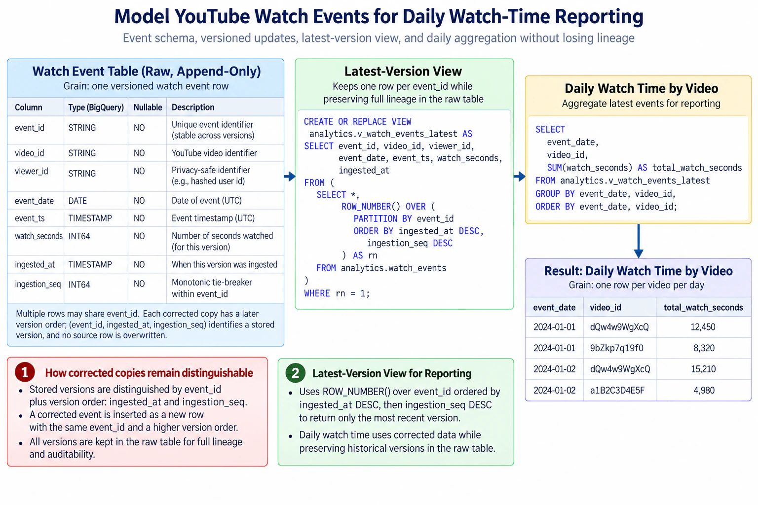
Define one watch-event row with event_id, video_id, privacy-safe viewer identifier, event_date, event timestamp, watch seconds, and ingested_at. State how corrected copies of the same event remain distinguishable and how a latest-version view supports daily watch time by video without discarding source lineage.

Short Interview Answer (30-60 seconds)

Store watch events append-only, with one row per event version. Keep event_id stable across corrections and order versions by ingested_at plus ingestion_seq. Build a latest-version view per event_id, then sum watch_seconds by event_date and video_id while retaining every raw version.

Detailed Explanation

See the Code while reading this explanation.

Each time someone watches a video, store one record describing that watch. If the record later needs a correction, add another copy instead of replacing the old one. Both copies keep the same event identity, while their version order tells us which copy is newer. This keeps the full history for checking and auditing. For reports, use only the newest copy of each watch. Then add the watched seconds for each video on each day. This gives corrected daily totals while keeping every earlier copy available.

Useful Questions to Ask the Interviewer
  1. Should event_date always represent the UTC reporting date?
  2. Can two corrected copies of the same event have the same ingested_at value?
  3. Is ingestion_seq guaranteed to increase within each event_id so timestamp ties are deterministic?
Model YouTube watch events for daily watch-time reporting. diagram
How to Explain It in an Interview

Assume BigQuery using GoogleSQL, matching the diagram. The raw table is analytics.watch_events, and its grain is one stored version of one logical watch event.

The raw schema contains event_id STRING, video_id STRING, viewer_id STRING, event_date DATE, event_ts TIMESTAMP, watch_seconds INT64, ingested_at TIMESTAMP, and ingestion_seq INT64. The diagram models these fields as required rather than nullable. event_id identifies the logical watch event and stays the same when that event is corrected. viewer_id is a privacy-safe viewer identifier. event_date is the agreed UTC reporting date, event_ts is the watch-event timestamp, watch_seconds is the measure being reported, and ingested_at records when that version was ingested.

Corrections are append-only. A corrected event is inserted as a new row instead of updating or deleting the earlier row. Multiple rows can therefore share the same event_id. Stored versions remain distinguishable by their version order: ingested_at and ingestion_seq. In this model, the combination of event_id, ingested_at, and ingestion_seq identifies a stored version. ingestion_seq is the monotonic tie-breaker within an event_id when ingestion timestamps are equal.

The latest-version view keeps one row per event_id. It applies ROW_NUMBER() partitioned by event_id and orders by ingested_at DESC, ingestion_seq DESC. The row with rn = 1 is the latest version. Using both ordering columns makes the selection deterministic when ingested_at values tie. The raw table still keeps all older versions, so no source lineage is discarded.

Daily reporting reads from this latest-version view rather than directly from every raw version. It groups by event_date and video_id and calculates SUM(watch_seconds). The result grain is one row per video per day. This prevents an original event and its corrected copy from both contributing to the daily total.

The main tradeoff is additional storage and version-selection work. Keeping every version increases raw-table size, and reporting must consistently use the latest-version view. In return, the model preserves full lineage and auditability while allowing daily watch-time reports to use corrected event values.

Technical Approach
  1. Declare the raw grain as one stored version of one logical watch event.
  2. Keep event_id stable across all corrected copies.
  3. Append a corrected version instead of overwriting the previous row.
  4. Assign ingested_at and a monotonic ingestion_seq to define version order.
  5. Rank rows within each event_id by ingested_at DESC, ingestion_seq DESC.
  6. Keep ROW_NUMBER() = 1 as the latest version.
  7. Group latest rows by event_date and video_id.
  8. Sum watch_seconds to produce one result row per video per day.
Practical Insights

The raw table grows whenever a new watch event or correction arrives because previous versions are retained. The latest-version view must rank versions belonging to the same event_id before selecting one. The daily query then groups the selected events by day and video. Compute cost depends on how much data BigQuery processes. Operationally, each correction needs a reliable version order. Maintenance stays simple because historical rows are never rewritten, but reporting must consistently use the latest-version view instead of summing the raw table directly.

Code
-- BigQuery GoogleSQL.
-- Raw-model assumption from the diagram: required event fields are non-null,
-- and ingestion_seq is a monotonic tie-breaker within each event_id.
CREATE
OR REPLACE VIEW analytics.v_watch_events_latest AS
SELECT
  event_id,
  video_id,
  viewer_id,
  event_date,
  event_ts,
  watch_seconds,
  ingested_at
FROM
  (
    SELECT
      we.*,
      -- Rank versions separately for each logical event.
      -- ingested_at chooses the newest ingestion time; ingestion_seq breaks timestamp ties.
      ROW_NUMBER() OVER (
        PARTITION BY
          event_id
        ORDER BY
          ingested_at DESC,
          ingestion_seq DESC
      ) AS rn
    FROM
      analytics.watch_events AS we
  )
  -- Result grain of the view: one latest stored version per event_id.
WHERE
  rn = 1;


-- Aggregate only latest logical events so corrected and older copies are not double-counted.
SELECT
  event_date,
  video_id,
  -- watch_seconds is additive across distinct latest watch events for a video and day.
  SUM(watch_seconds) AS total_watch_seconds
FROM
  analytics.v_watch_events_latest
  -- Result grain: one row per event_date and video_id.
GROUP BY
  event_date,
  video_id
  -- ORDER BY affects presentation only; it does not change the aggregation grain.
ORDER BY
  event_date,
  video_id;
Why Interviewers Ask This

This tests whether the candidate can define a clear event grain, preserve correction history, distinguish logical events from stored versions, select the latest version deterministically, and aggregate at the correct reporting grain without destroying source lineage.

Common interview mistakes

Common mistakes are overwriting corrected events and losing lineage; treating event_id as unique in the append-only raw table even though several versions can share it; ordering only by ingested_at when ties are possible; failing to maintain a deterministic ingestion_seq; summing the raw table and double-counting older versions; grouping at the wrong grain; or using an event date definition that does not match the agreed UTC reporting date.

Interview tip

State the grain first. Then separate logical-event identity from version identity: event_id identifies the watch event, while ingested_at plus ingestion_seq orders its stored versions. Finish by explaining that reporting reads the latest-version view while every historical version remains in the append-only raw table.

Interviewer may ask next
Why keep ingestion_seq if ingested_at already tells us which version is newer?

ingested_at normally establishes version order when every version has a different timestamp. If two versions of the same event share the same ingested_at, ordering only by that timestamp leaves a tie. ingestion_seq supplies a monotonic secondary order within event_id, so ROW_NUMBER() can select one latest version deterministically.

Why not update the original watch-event row when a correction arrives?

Updating the original row would make the current state simpler, but it would remove the earlier source version unless history were stored separately. The append-only model keeps every received version for lineage and auditing. The latest-version view gives reporting consumers the corrected current state without deleting historical versions.

3. Design a database schema for a multi-modal advertising platform.Data ModelingMediumGoogle

Question Details

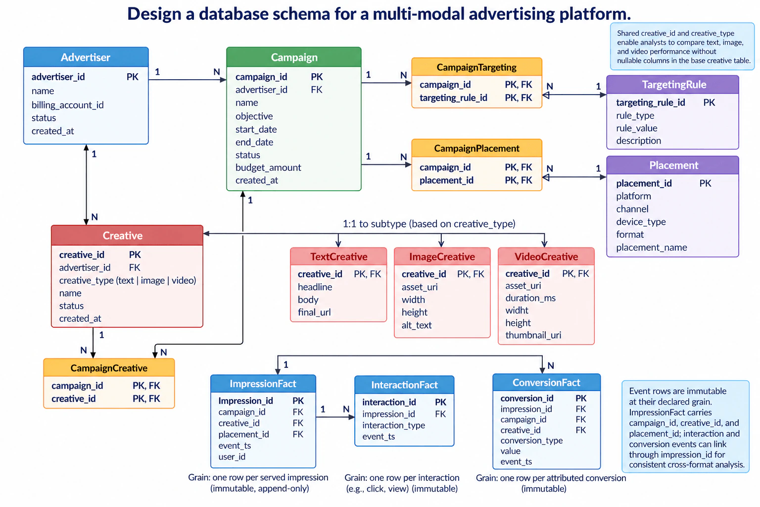
Model advertisers, campaigns, targeting rules, placements, and text, image, and video creatives together with impression, interaction, and conversion facts. Identify shared creative attributes and subtype-specific fields, many-to-many relationships, immutable event grains, and keys that let analysts compare formats without placing unrelated nullable columns in every creative record.

Short Interview Answer (30-60 seconds)

I would use shared Creative rows plus text, image, and video subtype tables, bridge tables for the three many-to-many campaign relationships, and immutable impression, interaction, and conversion facts. Shared creative_id and impression_id keys support consistent cross-format analysis without unrelated nullable creative columns.

Detailed Explanation

The platform must store who buys ads, which campaigns they run, where ads may appear, who should see them, and what happens after an ad is shown. Text, image, and video ads have some information in common but also need different details. The design should avoid putting many empty fields into every ad record. It should also keep each view, action, and completed outcome as a separate permanent record so reports can compare all ad formats consistently and trace later activity back to the original ad impression.

Useful Questions to Ask the Interviewer
  1. Can the same creative be used by multiple campaigns?
  2. Can targeting rules be reused by multiple campaigns?
  3. Can a campaign use multiple placements, and can a placement be shared by multiple campaigns?
  4. Must every interaction and attributed conversion reference an existing impression?
  5. Should impression, interaction, and conversion records remain immutable after ingestion?
Design a database schema for a multi-modal advertising platform. diagram
How to Explain It in an Interview

Start with the main business entities and state their cardinalities.

Advertiser has advertiser_id as its primary key. One advertiser can own many Campaign rows through Campaign.advertiser_id. One advertiser can also own many Creative rows through Creative.advertiser_id.

Campaign contains campaign_id, advertiser_id, name, objective, start_date, end_date, status, budget_amount, and created_at.

TargetingRule contains targeting_rule_id, rule_type, rule_value, and description. Campaign and TargetingRule are many-to-many, so CampaignTargeting is a bridge table. Its composite primary key is (campaign_id, targeting_rule_id), and both columns are foreign keys. Each Campaign can therefore have many CampaignTargeting rows, and each TargetingRule can appear in many CampaignTargeting rows.

Placement contains placement_id, platform, channel, device_type, format, and placement_name. Campaign and Placement are also many-to-many. CampaignPlacement resolves that relationship with the composite primary key (campaign_id, placement_id). The composite key also prevents the same campaign-placement association from being stored twice.

Creative is the shared parent entity. It contains creative_id, advertiser_id, creative_type, name, status, and created_at. creative_type identifies text, image, or video. Keeping creative_id and creative_type in this shared table gives analysts one consistent identity and format classification across all creative types.

Do not place every possible format-specific field in Creative. Instead, use subtype tables whose creative_id is both the subtype primary key and a foreign key to Creative. TextCreative stores headline, body, and final_url. ImageCreative stores asset_uri, width, height, and alt_text. VideoCreative stores asset_uri, duration_ms, width, height, and thumbnail_uri. Each Creative is modeled with the matching subtype for its creative_type. This avoids unrelated nullable fields such as duration_ms on a text creative or body on an image creative.

Campaign and Creative are many-to-many. CampaignCreative is the bridge table with composite primary key (campaign_id, creative_id), with both columns also serving as foreign keys. A campaign can use several creatives, and a creative can be reused by several campaigns.

Next, declare each event fact grain explicitly. ImpressionFact has exactly one row per served impression. impression_id is its primary key. campaign_id, creative_id, and placement_id are foreign keys that capture the serving context. event_ts records the event time, and user_id identifies the user when that identifier is available. The diagram treats these rows as immutable and append-only.

InteractionFact has one row per interaction event, such as a click or view. interaction_id is its primary key. impression_id is a foreign key to ImpressionFact, while interaction_type and event_ts describe the event. InteractionFact does not repeat campaign_id, creative_id, or placement_id. Those values are obtained by joining through impression_id, which keeps the interaction fact narrow and avoids inconsistent copies of the same serving context.

ConversionFact has one row per attributed conversion. conversion_id is its primary key. impression_id is a foreign key to the attributed ImpressionFact row. The table also stores campaign_id and creative_id as foreign keys, plus conversion_type, value, and event_ts. It does not store placement_id, so placement is recovered from the referenced impression. Because campaign_id and creative_id are also available through impression_id, they are redundant convenience keys in this fact. Ingestion or validation should keep them consistent with the referenced impression so the same conversion cannot claim conflicting campaign or creative context.

For cross-format reporting, start from the fact tables and use creative_id to join to Creative. creative_type then allows the same metric logic to compare text, image, and video. InteractionFact reaches that context through ImpressionFact. ConversionFact can use its direct creative_id and campaign_id while impression_id preserves attribution lineage and provides placement context.

The main tradeoff is normalization versus query convenience. Creative subtype tables eliminate unrelated null columns and keep format-specific attributes clean, but retrieving full subtype details requires an additional join. InteractionFact avoids duplicating campaign, creative, and placement keys, but analyses needing those fields must join to ImpressionFact. ConversionFact keeps campaign_id and creative_id for convenience, but those redundant keys require consistency checks against the referenced impression.

Technical Approach
  1. Identify the core entities: Advertiser, Campaign, TargetingRule, Placement, and Creative.
  2. Put only format-independent attributes in Creative and move text-, image-, and video-specific attributes into one-to-one subtype tables.
  3. Resolve Campaign-to-TargetingRule with CampaignTargeting, Campaign-to-Placement with CampaignPlacement, and Campaign-to-Creative with CampaignCreative.
  4. Give each bridge a composite primary key made from its two foreign keys so duplicate relationship rows are prevented.
  5. Declare immutable event grains: one ImpressionFact row per served impression, one InteractionFact row per interaction, and one ConversionFact row per attributed conversion.
  6. Use impression_id to connect interactions and conversions to their original impression context.
  7. Use creative_id and Creative.creative_type as the common analytical path for comparing text, image, and video formats.
  8. Validate redundant campaign_id and creative_id values on ConversionFact against the referenced ImpressionFact row.
Practical Insights

The normalized design uses more tables and therefore requires some extra joins. That increases query complexity slightly, but it avoids a large Creative table filled with fields that are meaningless for most formats. Bridge-table storage grows with the number of actual campaign-to-rule, campaign-to-placement, and campaign-to-creative relationships. Fact-table storage grows directly with advertising activity because every impression, interaction, and conversion is retained at its own immutable grain. Large analytical scans can therefore be expensive, so physical partitioning or clustering should be chosen later from real query patterns rather than assumed in the logical model.

Why Interviewers Ask This

This question tests whether the candidate can choose clean entity boundaries, model many-to-many relationships correctly, normalize subtype-specific data without creating sparse records, define unambiguous immutable event grains, and select keys that support reliable analytics across text, image, and video creatives. It also tests judgment about normalization, controlled denormalization, data integrity, and analytical usability.

Common interview mistakes

Common mistakes include putting all text, image, and video attributes into one wide Creative table with many unrelated nulls; modeling a many-to-many relationship as a single foreign key; omitting composite keys from bridge tables and allowing duplicate associations; mixing impressions, interactions, and conversions into one table with an unclear grain; adding a direct InteractionFact-to-ConversionFact relationship even though ConversionFact has no interaction_id; duplicating campaign, creative, and placement context in InteractionFact instead of using impression_id; assuming ConversionFact contains placement_id when the diagram requires placement to be obtained through ImpressionFact; allowing ConversionFact.campaign_id or creative_id to disagree with its referenced impression; and updating historical event facts instead of treating them as immutable records.

Interview tip

Lead with the three decisions that matter most: shared Creative plus subtype tables, bridge tables for many-to-many relationships, and explicit immutable event grains. Then trace one impression to an interaction or conversion and show how creative_id and creative_type support the same analytics across text, image, and video.

Interviewer may ask next
How would you report interactions by campaign, creative format, and placement when InteractionFact only stores impression_id?

Join InteractionFact to ImpressionFact on impression_id. ImpressionFact provides campaign_id, creative_id, and placement_id. Then join creative_id to Creative to obtain creative_type. The result can group the same interaction metric by campaign, placement, and text, image, or video format without adding those repeated context columns to InteractionFact.

Why keep campaign_id and creative_id in ConversionFact when impression_id can already reach them?

They are convenience fields that can make common conversion analysis simpler, while impression_id preserves the attribution link and supplies placement context. The tradeoff is redundancy. The ingestion pipeline or data-quality checks must verify that ConversionFact.campaign_id and creative_id match the campaign_id and creative_id on the referenced ImpressionFact row; otherwise reports could disagree depending on which path is used.

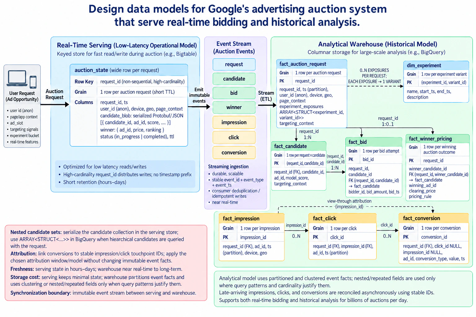
4. Design data models for Google's advertising auction system that serve real-time bidding and historical analysis.Data ModelingHardGoogle

Question Details

Separate the low-latency operational representation from the analytical warehouse for billions of auctions per day. Define grains and keys for request, candidate ad, bid, winner, pricing, impression, click, conversion, targeting context, and experiment; address nested candidate sets, attribution, freshness, storage cost, and the synchronization boundary between the serving and historical models.

Short Interview Answer (30-60 seconds)

Use a short-lived request-keyed operational record for the live auction and an immutable event stream as the synchronization boundary. In the warehouse, model request, candidate, bid, winner/pricing, impression, click, conversion, and experiment data at separate grains, with partitioning, clustering, optional attribution links, and idempotent late-event reconciliation.

Detailed Explanation

The main decision is to keep the live auction data separate from the long-term reporting data. During an auction, the system needs one small record that it can find and update very quickly. After each important action, it sends a permanent event to another system. Those events are later organized into separate records for requests, ads considered, bids, winners, views, clicks, purchases, and experiments. This keeps the live path fast while preserving enough history for reporting, learning, experiments, attribution, and delayed actions that may arrive later.

Useful Questions to Ask the Interviewer
  1. Does one request represent exactly one ad opportunity, or can a request contain several ad slots?
  2. Can a candidate receive more than one bid attempt during a request?
  3. Can one impression produce multiple click events, and can one click be associated with multiple conversions?
  4. Do we need both click-through and view-through conversion attribution?
  5. Can one request participate in multiple experiments at the same time?
  6. What freshness target is required for historical reporting: near-real-time, minutes, or hours?
  7. How long must raw event-level history be retained before it can be aggregated or expired?
Design data models for Google's advertising auction system that serve real-time bidding and historical analysis. diagram
How to Explain It in an Interview

I would start by separating the two workloads because their requirements are different.

The serving model handles the auction while it is happening. The analytical model stores durable history for reporting and analysis. An immutable event stream sits between them, so warehouse latency or failures do not become part of the bidding path.

1. Low-latency operational model

Use a wide operational record called auction_state with grain 1 row per auction request.

The row key is a non-sequential, high-cardinality request_id. The important property is that the key is directly addressable and does not begin with a monotonically increasing timestamp. That avoids a timestamp-led sequential-write hotspot and supports fast point reads and writes in a Bigtable-style keyed serving store.

The row contains request_id, timestamp, anonymized user_id, device, geography, page context, targeting information, experiment context, the serialized candidate collection, winner information, status, and TTL. The candidate collection is serialized, for example as Protobuf or JSON, rather than modeled as a native BigQuery-style repeated SQL structure in the serving store.

The approved model treats a request as one ad opportunity, so the visible request field is ad_slot. Serving state has short retention, measured in hours to days, because durable history belongs in the event stream and warehouse.

2. Synchronization boundary

Every important transition emits an immutable event. The stream carries request, candidate, bid, winner, impression, click, conversion, and experiment information.

Events have stable identity fields such as event_id, event_type, and event_ts. Consumers use stable event IDs for deduplication and idempotent writes, so duplicate delivery does not create duplicate analytical facts.

This event stream is the synchronization boundary. The operational store remains responsible for low-latency mutable state, while the analytical side can ingest and reconcile events asynchronously.

3. Analytical request and experiment model

fact_auction_request has grain 1 row per auction request and primary key request_id.

It contains request timestamp, anonymized user information, device, geography, page context, targeting context, and experiment exposures. Because one request can participate in zero or many experiments, the diagram represents experiment membership as ARRAY<STRUCT<experiment_id, variant_id>> instead of a single experiment column.

dim_experiment has grain 1 row per experiment variant with composite primary key (experiment_id, variant_id). Each exposure identifies exactly one experiment variant, while a request can have zero to many exposures.

4. Candidate grain

fact_candidate has grain 1 row per request × candidate with composite primary key (request_id, candidate_id).

It contains request_id, candidate_id, ad_id, model score, and targeting context. One request can therefore have many candidate rows.

This table represents ads considered for the auction. Keeping that grain separate is important because candidate evaluation and bid attempts are not necessarily the same business event.

5. Bid grain

fact_bid has grain 1 row per bid attempt with primary key bid_id.

It contains request_id, candidate_id, bidder identifier, bid amount, and bid timestamp. The pair (request_id, candidate_id) is a foreign key to fact_candidate.

The diagram models candidate to bid as 1:N, which allows a candidate to have multiple bid attempts. That avoids incorrectly forcing candidate selection and bidding into one fact grain.

6. Winner and pricing

fact_winner_pricing has grain 1 row per winning auction outcome and uses request_id as its primary key.

The relationship from request to winner is 1:0..1: one request can have no winner, or one winning outcome. This supports no-fill auctions instead of assuming every request succeeds.

The record contains winner_candidate_id, winning_ad_id, clearing_price, and pricing_rule. The winning candidate is referenced using the composite relationship (request_id, winner_candidate_id) back to fact_candidate.

7. Impression fact

fact_impression has grain 1 row per impression with primary key impression_id.

It contains request_id, ad_id, timestamp, device, and geography. The impression is a durable delivery event that occurs after the auction outcome rather than part of the mutable serving record.

8. Click fact

fact_click has grain 1 row per click with primary key click_id.

It contains request_id, impression_id, ad_id, and timestamp. One impression can produce zero to many click events, so the relationship from impression to click is 0..N on the click side.

9. Conversion fact and attribution

fact_conversion has grain 1 row per conversion with primary key conversion_id.

It contains request_id, nullable click_id, nullable impression_id, ad_id, conversion type, value, and timestamp. One click can be associated with zero to many conversions.

The nullable attribution references are important. A click-through conversion can reference a click. A view-through conversion can reference an impression without requiring a click. The diagram therefore includes an optional dashed impression-to-conversion view-through attribution path.

Attribution rules should not mutate the immutable source events. Persist stable impression and click touchpoint IDs, then apply the chosen attribution window or model during analytical processing. This allows the same historical events to be re-evaluated if attribution policy changes.

10. Nested candidate sets

The serving model serializes the candidate collection because its primary job is fast request-level state access.

In BigQuery, ARRAY<STRUCT<...>> can be useful when a request and its hierarchical candidates are normally read together. It is not automatically the best representation for every workload. The approved analytical design keeps a separate fact_candidate grain for candidate-level filtering, joining, and aggregation while acknowledging that nested or repeated fields can be used when query patterns justify them.

11. Freshness and late-arriving data

Serving state is current for the live auction and retained only briefly. The warehouse is near-real-time to long-term and is not placed directly in the bidding path.

Impressions, clicks, and conversions may arrive after their related request or winner events. Analytical consumers reconcile these late events asynchronously using stable identifiers. Duplicate events are handled through deduplication or idempotent writes rather than by assuming perfect delivery order or uniqueness.

12. Storage and query cost

Keep only the state required for the active auction in the serving store.

In the warehouse, partition event facts using appropriate event-time columns so time-bounded queries can avoid reading unrelated partitions. Use clustering when repeated filter or join patterns justify it. Use nested or repeated fields only when their query pattern and cardinality justify them.

These choices reduce scan cost, but none is a universal optimization. Older raw events can be retained according to business needs and summarized when long-term analysis no longer requires full event-level detail.

The final boundary is clear: the serving model owns low-latency mutable auction state, the immutable event stream carries changes, and the analytical warehouse owns durable historical facts, experiment analysis, attribution, late-event reconciliation, and large-scale historical queries.

Technical Approach
  1. Declare one auction request as the central business event and assign a stable, non-sequential, high-cardinality request_id.
  2. Store current auction state in a short-lived operational row keyed by request_id.
  3. Emit immutable events with stable event IDs for request, candidate, bid, winner, impression, click, conversion, and experiment activity.
  4. Treat the event stream as the synchronization boundary so warehouse processing cannot slow the serving path.
  5. Load request, candidate, bid, winner/pricing, impression, click, conversion, and experiment data into analytical structures with explicitly declared grains.
  6. Preserve composite relationships such as (request_id, candidate_id) and (experiment_id, variant_id).
  7. Model a winner as optional, experiment exposures as zero-to-many, impression-to-click as zero-to-many, click-to-conversion as zero-to-many, and conversion attribution references as nullable.
  8. Partition event facts and apply clustering or nested/repeated fields only when actual query patterns justify them.
  9. Reconcile late or duplicate events idempotently using stable identifiers instead of relying on arrival order.
Practical Insights

The live path performs direct request-level reads and writes, so work for one auction is driven mainly by that request's candidate and bid activity rather than by the size of all historical data. Warehouse storage grows with the number of request, candidate, bid, impression, click, and conversion records retained. Partitioning can reduce the amount of data scanned for time-bounded queries. Clustering can reduce scanned blocks for common filters or joins. Nested data can simplify request-with-children reads, while separate facts make candidate-level filtering, deduplication, late-event handling, and independent retention easier. The tradeoff is more warehouse joins in exchange for clearer grains and relationships.

Why Interviewers Ask This

This question tests whether a candidate can design two different data models for two different workloads without losing semantic consistency. The interviewer is looking for clear grains and keys, correct cardinalities, scalable serving access patterns, event-driven synchronization, nested-data judgment, experiment modeling, attribution handling, late-arriving-event processing, freshness tradeoffs, and storage-cost awareness at very large scale.

Common interview mistakes

Common mistakes are using one schema for both serving and analytics; putting long historical data in the live auction record; prefixing serving keys with monotonically increasing timestamps; assuming high cardinality alone guarantees perfect distribution; combining candidate and bid grains; assuming every request has a winner; using experiment_id alone when the experiment dimension grain is variant-level; allowing only one experiment per request; requiring every conversion to have a click; limiting an impression to one click or a click to one conversion; changing immutable events when attribution rules change; assuming events always arrive once and in order; and treating partitioning, clustering, or nested fields as universally better regardless of query patterns.

Interview tip

Start by drawing the synchronization boundary. Then state every table's grain before listing fields. Explicitly call out the important cardinalities: many candidates per request, many bid attempts per candidate, zero-or-one winner per request, zero-or-many experiment exposures, zero-or-many clicks per impression, zero-or-many conversions per click, and optional impression or click attribution. Finish with freshness and storage tradeoffs.

Interviewer may ask next
How would you handle late or duplicate impression, click, and conversion events?

Give every event a stable event_id and event timestamp. Consumers use the stable event ID for deduplication or idempotent writes and do not assume events arrive exactly once or in order. A late impression, click, or conversion is inserted or reconciled using its stable primary key and its request, impression, or click references. Attribution can then be recomputed from durable touchpoint IDs without changing the original immutable event.

When would you keep candidates nested in the request instead of using a separate candidate fact table?

Use a nested ARRAY<STRUCT<...>> representation when most analytical queries read the request together with its bounded candidate collection. Use a separate fact_candidate when analysts frequently filter, aggregate, join, or retain candidate rows independently. The approved design serializes the candidate collection in the serving record and uses a separate candidate fact in the warehouse, while allowing nested or repeated fields only when the BigQuery query patterns and cardinality justify them.

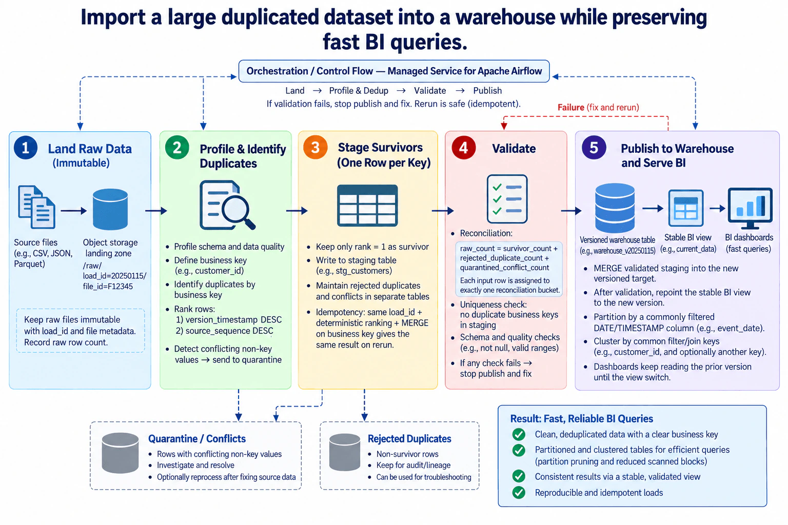
5. Import a large duplicated dataset into a warehouse while preserving fast BI queries.Data PipelinesEasyGoogle

Question Details

Design landing, profiling, deterministic duplicate identification, survivor selection, staging, and warehouse publication for a large import. State the business key, version or tie-break rule, treatment of conflicting duplicates, partition and clustering layout, reconciliation totals, and how the load remains idempotent while dashboards continue to query a stable published version.

Short Interview Answer (30-60 seconds)

I would land the source files unchanged, profile them, deduplicate by a business key using a deterministic version and tie-break rule, and stage one survivor per key. Conflicts go to quarantine, rejected duplicates stay auditable, and counts reconcile before publication. I would MERGE into a new versioned warehouse target and switch the stable BI view only after validation. The trade-off is extra storage and publication work for stronger isolation, repeatability, and fast BI queries.

Detailed Explanation

The goal is to move a very large set of repeated records into an analytics system without letting duplicates or conflicting values produce wrong reports. I would first keep the original input unchanged so it can be checked again. Then I would inspect the data, decide which repeated record should win, separate records that cannot be resolved safely, and prove that every input record is accounted for. Only after those checks pass would I make the new version visible to reporting users. This keeps reports stable while the new load is prepared.

Useful Questions to Ask the Interviewer
  1. What fields form the business key that identifies the same real-world record?
  2. Which field represents the preferred version, and what deterministic tie-break field should be used when versions match?
  3. Is source_sequence guaranteed to break any remaining tie for the same business key and version?
  4. Which non-key differences should be treated as conflicts instead of automatically choosing a survivor?
  5. Which DATE or TIMESTAMP column is commonly used by BI filters, and which columns are common filter or join keys?
Import a large duplicated dataset into a warehouse while preserving fast BI queries. diagram
How to Explain It in an Interview
1. Land the import unchanged

I would start by landing every source file in an immutable object-storage landing zone. The diagram records a load_id, file_id, and the raw row count. The data path is source files to object storage. Managed Service for Apache Airflow controls the workflow order, but orchestration is separate from the business-data path. Keeping the landing data unchanged gives me a repeatable input boundary for investigation and reruns.

2. Profile and identify duplicates deterministically

Next, I would profile schema and data quality and define the business key, such as customer_id in the diagram. Rows with the same business key are duplicate candidates. I would rank them by version_timestamp DESC and then source_sequence DESC. Rank 1 is the survivor. This is deterministic only if that ordering fully breaks ties, so I would confirm that source_sequence is unique enough for that purpose. If important non-key values conflict, I would send those rows to the quarantine/conflicts path rather than silently choosing a value.

3. Stage one survivor per key

The survivor rows go to a staging table such as stg_customers. Non-survivor duplicates are retained separately as rejected duplicates for audit and troubleshooting. The idempotency boundary uses the same load_id, the same business key, and the same deterministic ranking and MERGE rules. If the workflow is rerun for the same input, it should reproduce the same staged business result instead of creating another copy. Quarantined conflicts remain outside the normal survivor path until they are investigated and corrected.

4. Validate and reconcile before publication

Before anything becomes BI-visible, I would validate the staged result. The diagram checks uniqueness of business keys, schema and quality rules, and row-count reconciliation. The required reconciliation is raw_count = survivor_count + rejected_duplicate_count + quarantined_conflict_count, with each input row assigned to exactly one bucket. If a check fails, publication stops. The failure path is to correct the problem and rerun; task completion alone is not treated as proof that the data is correct.

5. Publish a new version and switch the stable BI view

After validation succeeds, I would MERGE the validated staging data into the new versioned warehouse target, for example warehouse_v20250115. Dashboards continue reading the prior published version through the stable BI view while this target is prepared. After the new version passes validation, I repoint the stable BI view to it. That view switch is the consumer-visibility boundary. The important design decision is that dashboards do not query the in-progress target, so they do not see a partial load.

6. Keep BI queries fast and reruns reproducible

For the published warehouse table, I would partition by a commonly filtered DATE or TIMESTAMP field such as event_date. I would cluster on common filter or join keys such as customer_id, with another useful key only when the BI access pattern supports it. This allows the warehouse to avoid scanning unnecessary partitions and can reduce blocks scanned for clustered filters. Managed Service for Apache Airflow coordinates the land, profile and deduplicate, validate, and publish sequence. If validation fails, the load is corrected and rerun with the same deterministic rules and load identity.

Technical Approach
  1. Land every source file unchanged and record load_id, file_id, and raw row count.
  2. Profile schema and data quality.
  3. Define the business key.
  4. Group duplicate candidates by that key.
  5. Rank them by version_timestamp DESC, then source_sequence DESC, assuming that ordering fully breaks ties.
  6. Keep rank 1 as the survivor.
  7. Route important conflicting non-key values to quarantine and retain other non-survivors as rejected duplicates.
  8. Write survivors to staging.
  9. Verify business-key uniqueness, schema and quality rules, and raw_count = survivor_count + rejected_duplicate_count + quarantined_conflict_count.
  10. Stop publication if validation fails.
  11. MERGE validated staging into the new versioned warehouse target.
  12. Repoint the stable BI view only after validation succeeds.
  13. Partition by the chosen DATE/TIMESTAMP field and cluster by common BI filter or join keys.
Practical Insights

The benefit is strong correctness and stable BI access during a large import. Immutable landing makes reruns and investigation easier, while deterministic ranking prevents the same duplicate set from producing different survivors. A separate versioned warehouse target also keeps dashboards away from data that is still being prepared. The downside is extra storage for raw, staging, rejected, quarantined, and versioned data, plus more processing and one additional publication step. Ranking and MERGE operations can also be expensive on a large load. Partitioning and clustering reduce work only when they match real BI filter patterns. We accept the extra storage and workflow complexity because correctness, repeatability, and stable dashboard results are more important than exposing an unfinished import earlier.

Why Interviewers Ask This

This question tests whether a Data Engineer can protect correctness and BI performance at the same time. The interviewer wants to see whether you can define the business key, make duplicate selection deterministic, isolate conflicting records, reconcile every input row, design an idempotent rerun, and control when new data becomes visible. It also tests whether you understand publication boundaries and how partitioning and clustering support analytical query performance without weakening correctness.

Common interview mistakes

Common mistakes are deduplicating without defining the business key, choosing an arbitrary survivor, using a version field without a complete deterministic tie-break rule, silently dropping conflicting duplicates, and failing to reconcile every input row. Another mistake is publishing directly into the BI-visible version while the import is still being validated. Reruns are also unsafe when they create additional copies instead of reusing the same load identity and deterministic matching rules. For performance, choosing partition or clustering columns that do not match real BI filters and joins can add complexity without reducing useful query work.

Interview tip

Explain the design as two concerns: first make the imported data correct, then make the validated version visible. State the business key and survivor rule early. Explicitly account for survivors, rejected duplicates, and quarantined conflicts. Finish by explaining the stable-view switch, idempotent rerun behavior, and why the partition and clustering keys match BI access patterns.

Interviewer may ask next
What would you change if the import failed after staging was written but before the stable BI view was switched?

I would keep the current BI-visible version unchanged and rerun from the same load boundary. The changed requirement is recovery after some internal work has already completed. The affected areas are staging, validation, the versioned warehouse target, and orchestration state. I would reuse the same load_id, business key, and deterministic ranking rule, then repeat the staging or MERGE work that did not reach a valid publication point. Because the same input and ranking rules are reused, the rerun should reproduce the same business result rather than create another copy. I would rerun uniqueness, schema, quality, and reconciliation checks before publication. The stable BI view would still point to the prior validated version until all checks pass, so dashboards remain isolated from partial work. Quarantined conflicts and rejected duplicates remain separately auditable. The main downside is repeated compute and longer recovery time for a large load, but the original architecture and consumer-facing behavior stay unchanged.

How would you handle duplicate records that have the same business key and version but different non-key values?

I would not choose between important conflicting values arbitrarily. The changed requirement is duplicate resolution when the business key and version alone are insufficient. The profiling and deduplication stage still applies the deterministic tie-break rule shown in the design, but I would first confirm that source_sequence fully breaks the remaining tie. If important non-key values still represent a true conflict, those input rows belong in the quarantine/conflicts path rather than the normal survivor path. They must be counted in quarantined_conflict_count so reconciliation still assigns every raw input row to exactly one bucket. After the conflict is investigated and corrected through the shown recovery path, I would rerun using the same load_id and deterministic rules. Validation must again check uniqueness, schema, quality, and totals before a new version becomes BI-visible. The downside is slower publication when conflicts require investigation, but that is preferable to silently publishing the wrong business value.

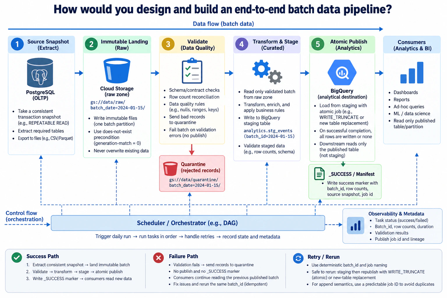
6. How would you design and build an end-to-end batch data pipeline?Data PipelinesEasyGoogle

Question Details

Start with a named source and daily analytical destination, then specify extraction boundary, immutable landing, validation, transformation, staging, atomic publication, orchestration, and consumer handoff. Include the batch partition, completion marker, retry and rerun behavior, rejected-record path, observability, and the rule that prevents downstream readers from seeing a partially written result.

Short Interview Answer (30-60 seconds)

I would take a consistent daily snapshot from PostgreSQL, store that batch immutably in Cloud Storage, validate it, transform the accepted data into a BigQuery staging table, and publish it atomically. A scheduler or orchestrator runs those steps in order and records their state. Invalid records go to quarantine. Consumers read only the published table, never staging, so failed runs cannot expose partial data. The trade-off is stronger correctness at the cost of extra staging, validation, and storage.

Detailed Explanation

The goal is to move one day's business data from the operational database into a reliable reporting destination without showing incomplete results. I would first take one consistent view of the source and save that day's copy separately so it can be checked or processed again later. Before making the new result available, I would check that the data is complete and sensible. Bad records would be separated instead of silently ignored. Only after all required checks and processing finish would the new result replace the old visible result.

Useful Questions to Ask the Interviewer
  1. Which PostgreSQL tables are required in the daily snapshot, and what source consistency boundary should the batch use?
  2. Is the BigQuery analytical result a full daily replacement, or does it use append semantics?
  3. Which schema, row-count, and business-rule checks must block publication?
  4. Should one invalid record quarantine only that record, or should certain validation failures reject the whole batch?
  5. How long should immutable raw batches and quarantine data be retained?
How would you design and build an end-to-end batch data pipeline? diagram
How to Explain It in an Interview
1. Extract one consistent PostgreSQL batch

I would start by defining one daily batch identity, such as batch_date=2024-01-15. The source is PostgreSQL OLTP. I take a consistent transaction snapshot, for example with REPEATABLE READ, so the required tables are read from one stable source view instead of changing independently during extraction. I export the required data to files such as CSV or Parquet. That snapshot boundary matters because later validation and reruns should refer to the same logical input.

2. Land the raw batch immutably

The exported files move to the Cloud Storage raw zone under gs://data/raw/batch_date=2024-01-15/. This is the immutable landing boundary. Existing objects for that batch are not overwritten. Cloud Storage's ifGenerationMatch=0 precondition corresponds to the diagram's generation-match = 0 rule: a write succeeds only when no live object with that name already exists. Keeping the original input gives the pipeline a stable rerun source and an audit trail.

3. Validate before transformation

Next I validate the landed batch. The checks shown are schema or contract checks, row-count reconciliation, and business rules such as null, range, and key validation. Records that fail applicable record-level checks are sent to gs://data/quarantine/batch_date=2024-01-15/. A blocking validation failure stops publication. Task completion alone is not enough because a task can execute successfully while its data is unacceptable. The quality gate decides whether the batch can continue.

4. Transform into BigQuery staging

Only the validated batch moves into transformation. The processing step reads the validated raw batch, cleans or enriches it, applies the required business rules, and writes the result to the BigQuery staging table analytics.stg_events for batch_id=2024-01-15. I then validate staged data again, including row-count and schema checks. Consumers never read this staging table. Staging isolates work in progress from the currently published analytical result.

5. Publish atomically and mark completion

After staging passes its checks, I publish the result with one BigQuery job using the shown replacement approach, such as WRITE_TRUNCATE. BigQuery applies the successful load or query destination update atomically, so consumers continue seeing the previous published result until the new job completes. They never read a partially written result. Only after publication succeeds does the pipeline write the _SUCCESS or manifest record containing the batch ID, row counts, source snapshot information, and publication job ID. The marker records completion; it is not the mechanism that makes the table update atomic.

6. Orchestrate, observe, and rerun safely

A scheduler or orchestrator triggers the daily workflow, runs tasks in dependency order, handles retries, and records workflow state and metadata. Observability stays outside the business-data path and records task status, batch ID, row counts, duration, validation results, publication job ID, and lineage. If validation or publication fails, there is no new _SUCCESS marker and consumers keep reading the previous published batch. A rerun reuses the deterministic batch ID and job naming, rebuilds staging, and republishes safely. For append semantics, deterministic publication job identity helps prevent duplicate work when retrying an uncertain job submission.

Technical Approach
  1. Assign the daily run a deterministic batch ID such as the batch date.
  2. Take a consistent PostgreSQL transaction snapshot and export the required tables.
  3. Write files once to the immutable Cloud Storage batch partition using ifGenerationMatch=0 for each object that must not already exist.
  4. Validate schema, row counts, and business rules; route rejected records to the matching quarantine partition and block publication on required failures.
  5. Transform only validated data and write it to the BigQuery staging table for that batch ID.
  6. Validate the staged output before publication.
  7. Publish with one atomic BigQuery replacement job so consumers never read staging or partial output.
  8. Write the _SUCCESS or manifest record only after successful publication.
  9. Record task state, counts, duration, validation results, publication job ID, and lineage.
  10. On retry or rerun, reuse the same batch identity and rebuild staging rather than changing the immutable raw input.
Practical Insights

The benefit is strong correctness and easy recovery. An immutable raw batch gives us a stable source for reruns, while staging and atomic publication stop readers from seeing incomplete data. The downside is extra storage and extra work because the same batch may exist in raw, staging, quarantine, and published forms. Validation also adds processing time before reports become available. Larger daily batches increase extraction, transformation, and publication time, while smaller or more frequent batches increase orchestration overhead. We accept this because the requirement favors a dependable daily analytical result over very low latency. The main operational costs are source reads, Cloud Storage, transformation work, BigQuery jobs, retries, and metadata for tracing each batch.

Why Interviewers Ask This

Interviewers ask this to test whether you can turn a simple data movement requirement into a reliable production pipeline. They want to see whether you separate data flow from orchestration, define clear batch boundaries, validate before publication, isolate rejected records, and make retries safe. The strongest answers also explain the visibility boundary: consumers must never see a half-written analytical result, even when a task fails or the same batch is rerun.

Common interview mistakes

Common mistakes are reading PostgreSQL tables without one consistent snapshot boundary, overwriting the raw batch, treating task success as proof that the data is correct, silently dropping rejected records, letting consumers query the staging table, and writing directly to the published destination in a way that exposes partial results. Another mistake is writing the _SUCCESS marker before BigQuery publication actually completes. Reruns can also create duplicate business results if batch or publication identity changes unexpectedly. Finally, monitoring should observe the pipeline; it should not be described as carrying or transforming the business data.

Interview tip

Explain the pipeline as two separate flows. Business data moves from PostgreSQL to immutable raw storage, validation, staging, publication, and consumers. Orchestration controls when those steps run and records their state. Spend extra time on the publication boundary: consumers read only the atomically published table, while a failed run leaves the previous result visible.

Interviewer may ask next
How would you handle a historical backfill for several past batch dates without damaging the current published result?

I would keep the same architecture and run each historical date as its own deterministic batch instead of mixing it with the current daily run. The requirement that changes is the input range: the orchestrator receives explicit historical batch IDs rather than only today's batch. For each date, I would reuse its immutable Cloud Storage raw partition when it already exists, run the same schema, row-count, and business-rule validation, and rebuild the corresponding BigQuery staging result. Rejected records would still go to that date's quarantine partition.

Publication must remain isolated. I would not let a backfill expose partially rebuilt data or overwrite unrelated current results. Each historical batch must pass staging validation and the same atomic publication boundary before becoming visible. The orchestrator records backfill task state separately so failures can be retried by batch ID. Recovery is verified with row counts, validation results, the publication job ID, and the completion marker. The downside is additional compute and storage use, so I would limit backfill concurrency rather than allowing historical runs to compete freely with the normal daily pipeline.

What would you change if some records fail validation but the business still wants the valid records published?

I would keep the same source, immutable landing, transformation, staging, publication, orchestration, and consumer boundaries, but make the validation contract explicitly distinguish record-level rejection from batch-level failure. Valid records would continue to transformation, while records failing permitted record-level rules would move to gs://data/quarantine/batch_date=.../. Schema failures, missing required inputs, or failed reconciliation rules that make the entire batch untrustworthy would still block publication.

The validation step would reconcile accepted and rejected records against the landed input so records cannot silently disappear. Only accepted data would reach the BigQuery staging table, and that staged output would still have to pass its checks before atomic publication. Consumers would continue reading only the published table. The completion manifest would be written only after publication succeeds, while validation results remain available through observability. If rejected data is corrected, rerunning with the same deterministic batch identity preserves recovery behavior. The downside is that the published batch may contain fewer accepted records than the source snapshot, so the rejection policy and reconciliation results must be explicit.

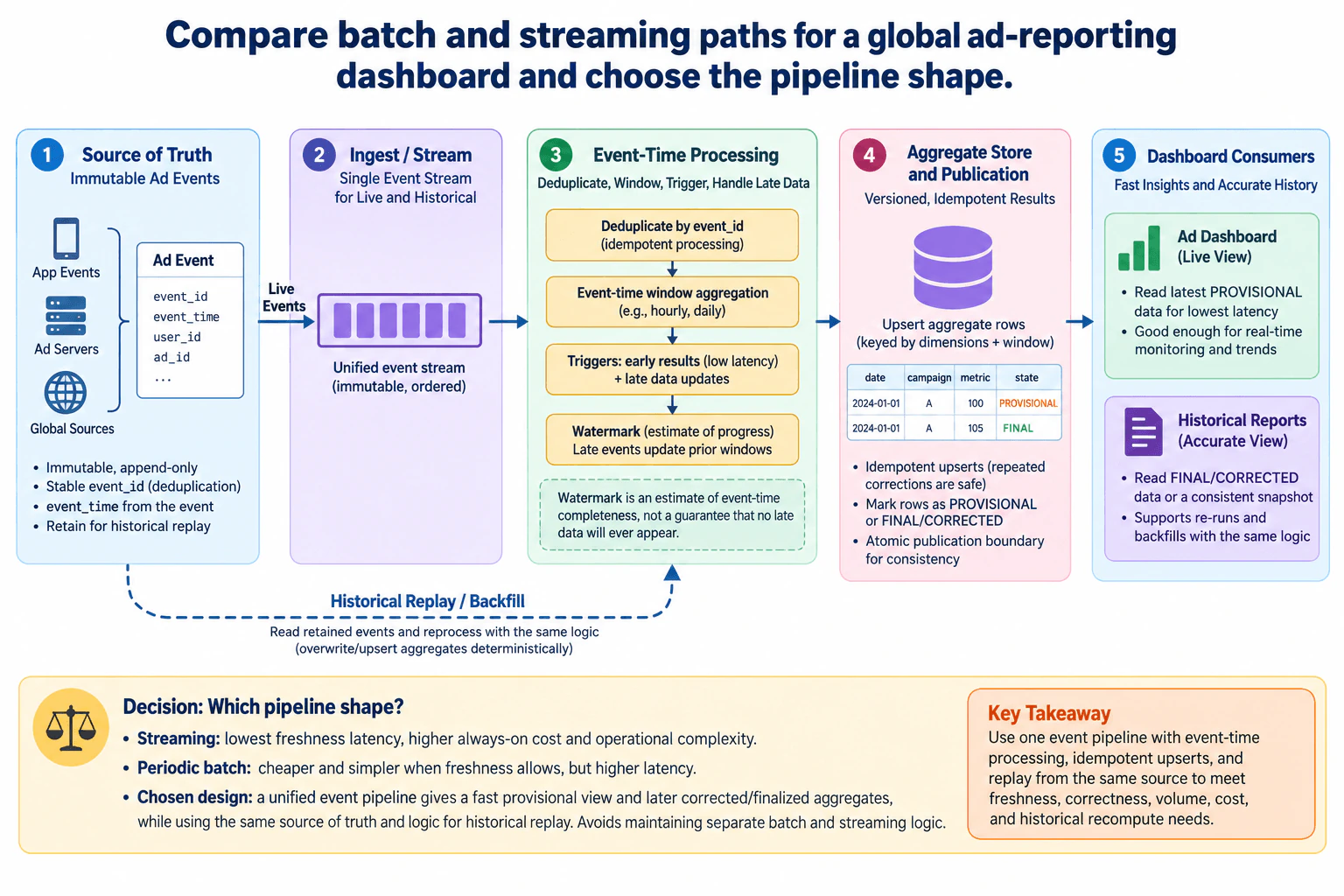
7. Compare batch and streaming paths for a global ad-reporting dashboard and choose the pipeline shape.Data PipelinesMediumGoogle

Question Details

Use explicit freshness, correctness, volume, cost, and historical-recompute requirements to decide between periodic batches, continuous processing, or one unified event pipeline. Define source of truth, window finalization, late corrections, backfills, duplicate handling, aggregate publication, and how consumers avoid discrepancies between a fast provisional view and a corrected historical view.

Short Interview Answer (30-60 seconds)

I would use one unified event pipeline backed by retained immutable ad events. Live events are deduplicated by event_id, aggregated in event-time windows, and published first as provisional results, then corrected when late data arrives. Idempotent upserts make repeated processing safe. The dashboard gets low latency, historical reports read corrected data, and backfills replay the same source through the same logic. The trade-off is higher always-on streaming cost and operational complexity.

Detailed Explanation

The goal is to show recent advertising numbers quickly without creating two different versions of the truth. Recent numbers may change because some events arrive late, while historical reports need stable corrected results. We also need a safe way to rebuild old reporting periods. The best shape is one shared flow that keeps the original events, produces an early view for speed, and later publishes corrected results. This avoids maintaining separate live and historical calculation logic that can slowly produce different answers.

Useful Questions to Ask the Interviewer
  1. How fresh must the live dashboard be: seconds, minutes, or is a scheduled delay acceptable?
  2. How long can events arrive late before a reporting window stops receiving normal late updates?
  3. Must historical reports always show corrected data, or may users explicitly request a provisional view?
  4. How much retained event history is required for replay and historical recomputation?
  5. What event volume must the pipeline sustain, and is lower cost more important than continuous freshness?
Compare batch and streaming paths for a global ad-reporting dashboard and choose the pipeline shape. diagram
How to Explain It in an Interview
1. Keep immutable ad events as the source of truth

I would start with one durable history of ad events. The diagram shows app events, ad-server events, and other global sources producing an Ad Event with fields such as event_id, event_time, user_id, and ad_id. The events are append-only and retained for historical replay. event_id is stable and supports duplicate detection. event_time represents when the event actually happened. Both live processing and later recomputation therefore begin from the same retained source instead of from separately maintained datasets.

2. Use one event stream for live and historical processing

Live events enter a unified event stream. I would not maintain one set of business rules for streaming and another for batch recomputation. Current events and retained events should pass through the same processing logic. The diagram describes the stream as immutable and ordered. In a real implementation, I would only rely on ordering within the ordering scope actually provided by the stream, not assume a global ordering guarantee. This shape supports continuous freshness while preserving a replay path for historical recomputation.

3. Deduplicate and aggregate by event time

The processing stage first deduplicates using event_id so repeated delivery or replay does not create repeated business results. It then groups events into event-time windows, such as hourly or daily reporting windows. Early triggers can emit a low-latency provisional aggregate before all expected events have arrived. A watermark is an estimate of event-time progress and completeness. It is not proof that no additional late event will ever appear.

4. Finalize windows with an explicit late-data policy

Late events can update earlier windows while those windows are still open for normal corrections. A window becomes FINAL/CORRECTED only when the chosen finalization policy says routine late updates are finished. The policy can use watermark progress together with an allowed correction period, without assuming that the watermark guarantees absolute completeness. If an event arrives after normal finalization, the retained source still allows a controlled historical replay or backfill. This gives the fast view low latency without pretending that an early answer is permanently correct.

5. Publish aggregates idempotently and consistently

The Aggregate Store contains rows keyed by reporting dimensions and window. Repeated corrections use idempotent upserts, so processing the same logical update again does not create extra aggregate rows. Publication needs a consistent visibility boundary so consumers do not observe a partially updated state. Each published result is marked PROVISIONAL or FINAL/CORRECTED. That state is part of the serving contract and tells consumers whether the value may still change.

6. Give each consumer the correct consistency view

The Ad Dashboard reads the latest PROVISIONAL data because its priority is low latency and trend visibility. Historical Reports read FINAL/CORRECTED data or a consistent corrected snapshot because their priority is accuracy. Both consumers depend on the same underlying aggregate pipeline. They avoid discrepancies by selecting data according to the explicit publication state rather than by using two independent calculation systems.

7. Choose the pipeline shape from freshness, volume, cost, and recompute needs

Streaming is the better fit when freshness must be low and global event volume is continuous because work is processed as events arrive. Its downside is higher always-on cost and operational complexity. Periodic batch is simpler and cheaper when scheduled freshness is acceptable, but it concentrates processing into batch windows and increases result latency. For this dashboard, I would choose the unified event pipeline because it provides fast provisional results, corrected historical results, duplicate-safe updates, and historical replay from the same retained source and business logic.

Technical Approach
  1. Define the immutable Ad Event contract with stable event_id and event_time.
  2. Retain events so the same source supports live processing and historical replay.
  3. Send current events through one unified event stream.
  4. Deduplicate events by event_id before aggregation.
  5. Aggregate by event-time windows and emit early provisional results when low latency is required.
  6. Use watermark progress and the late-data policy to update earlier windows when delayed events arrive.
  7. Mark a window FINAL/CORRECTED only when the chosen finalization policy says routine late corrections are complete.
  8. Upsert aggregate rows idempotently, keyed by reporting dimensions and window.
  9. Publish results through a consistent visibility boundary with an explicit PROVISIONAL or FINAL/CORRECTED state.
  10. Let the live dashboard read provisional data and historical reports read corrected data.
  11. For backfills, replay retained events through the same processing logic and deterministically update the affected aggregates.
Practical Insights

The benefit is that one event pipeline gives low-latency reporting and still supports accurate historical recomputation with the same business logic. The downside is higher always-on compute cost and more operational complexity than a scheduled batch job. Deduplication and late-event handling also require state, which consumes storage and processing resources. Waiting longer before finalizing a window can improve completeness, but stable results arrive later. Retaining more source history makes replay and backfill easier, but increases storage cost. Batch is cheaper and simpler when freshness can wait. We accept the streaming complexity here because the dashboard needs fast results, while shared logic and retained events reduce the risk that live and historical calculations drift apart.

Why Interviewers Ask This

This question tests whether a candidate can choose a pipeline shape from business requirements instead of automatically choosing batch or streaming. The interviewer wants to see judgment around freshness, correctness, event volume, cost, late data, duplicate handling, event-time windows, safe publication, and historical recomputation. It also tests whether the candidate can keep one source of truth, separate provisional from corrected results, and support replay without creating separate business logic that can drift.

Common interview mistakes

Common mistakes include building separate batch and streaming implementations that eventually calculate different numbers; using processing time when the business metric should follow event time; treating a watermark as proof that no more late data can arrive; failing to define when a window becomes FINAL/CORRECTED; publishing early aggregates without clearly labeling them PROVISIONAL; assuming transport delivery guarantees automatically prevent duplicate business results; failing to make aggregate updates idempotent; allowing live and historical consumers to interpret changing rows without a publication-state contract; assuming global ordering without a supported ordering scope; and building backfills from already aggregated data instead of replaying retained source events through the same logic.

Interview tip

Start with the decision: one retained source of truth and one unified event-processing path. Then explain why the dashboard is allowed to read PROVISIONAL data while historical reports require FINAL/CORRECTED data. Walk left to right through deduplication, event-time windows, watermarks, late updates, window finalization, idempotent publication, and replay. Finish with the trade-off: streaming buys freshness and continuous processing, while periodic batch is cheaper and simpler when the freshness requirement allows it.

Interviewer may ask next
What would you change if the dashboard no longer needed near-real-time freshness and could be updated every few hours?

I would reconsider the execution mode, but I would keep the same immutable source of truth and the same business aggregation logic. The changed requirement is freshness: if a few hours of delay is acceptable, periodic batch becomes much more attractive because continuous processing is no longer necessary. A batch run can read the retained events for the required reporting periods, deduplicate by event_id, apply the same event-time aggregation rules, and publish results through the same Aggregate Store contract.

The biggest simplification is that the dashboard may no longer need frequent PROVISIONAL publications. It can wait for the scheduled publication boundary and read the corrected batch result. Idempotent upserts should remain so reruns and backfills are safe. Retained source events should also remain because historical recomputation is still required.

Correctness does not weaken: the source contract, duplicate handling, finalization rules, publication consistency, and replay path stay intact. The downside is higher data latency. I would choose this version only because the freshness requirement explicitly allows that trade-off.

How would you handle a large historical backfill without creating different numbers from the live dashboard?

I would replay the retained immutable events through the same processing logic instead of creating a separate backfill calculation. The requirement that changes is the amount of historical data being processed, not the business rules. The backfill reads the required historical event range, applies the same event_id deduplication and event-time window aggregation, and deterministically upserts the same aggregate keys used by live processing.

The affected historical windows should be handled as a controlled replay so consumers do not observe uncontrolled partial updates. Publication still uses the same consistent visibility boundary, and the corrected results become FINAL/CORRECTED when the replayed updates are ready to publish. Because the sink operations are idempotent, repeating the backfill should update the intended logical result instead of multiplying it.

Recovery means rerunning the required retained-event range through the same logic and verifying the affected windows before publication. The main downside is temporary compute and storage pressure. The source contract, dashboard behavior, historical-report contract, and normal live path otherwise remain unchanged.

8. Design the YouTube metadata and engagement pipeline so schema changes do not break streaming dashboards or batch machine learning.NEWData PipelinesHardGoogle

Question Details

Combine mutable content metadata with high-volume engagement events under versioned producer contracts. Specify compatibility checks, dual-read or dual-write rollout, raw retention, stream and batch consumers, point-in-time joins, quarantine, late corrections, feature and dashboard publication, consumer ownership, backfill strategy, and rollback after an incompatible change.

Short Interview Answer (30-60 seconds)

The big picture is to protect consumers with versioned producer contracts and a compatibility gate. Metadata and engagement events keep their schema version and are retained in immutable raw storage. During a staged rollout, streaming and batch readers can handle vN and vN+1. Bad records are quarantined, late data can be replayed or backfilled, dashboards publish validated tables, and ML publishes point-in-time-correct features. The trade-off is extra migration and storage complexity in exchange for safer schema evolution.

Detailed Explanation

The goal is to let video information and viewer activity change over time without suddenly breaking live reports or the data used to train models. Every change gets a clear version and is checked before release. The original input is kept so the system can rebuild results later. Old and new formats can run together for a short migration period. Bad input is separated instead of silently accepted. If a new change causes trouble, the system can return to the earlier version and rebuild correct outputs from saved history.

Useful Questions to Ask the Interviewer
  1. Which schema changes must be supported during migration: only additive changes, or some incompatible changes too?
  2. How long should raw metadata and engagement events be retained for replay and model backfills?
  3. How late can engagement events or metadata corrections arrive?
  4. Which consumer team must approve readiness before a schema migration finishes?
Design the YouTube metadata and engagement pipeline so schema changes do not break streaming dashboards or batch machine learning. diagram
How to Explain It in an Interview
1. Define the versioned producer contract

I would start with one versioned contract for the two producer types shown in the diagram: mutable video metadata and high-volume engagement events. Metadata carries a schema version and effective_from/effective_to history because its values can change over time. Engagement events carry their schema version, event_time, and identifiers such as user_id and video_id. The contract defines allowed revisions and backward or forward compatibility rules. This gives every downstream reader an explicit version boundary instead of letting producer changes appear without warning.

2. Gate changes before they reach the pipeline

The next step is the Compatibility Gate in CI. It validates the schema definition, including syntax, types, and required fields, and then checks cross-version compatibility. If the change is incompatible, the release is rejected or quarantined and vN stays active. If it is compatible, vN+1 enters a staged rollout. During that rollout, vN and vN+1 can coexist through dual-read, dual-write, or a gradual percentage rollout. If a problem is detected, the control path rolls back to vN.

3. Keep immutable raw history

Compatible input moves into immutable raw storage. The system keeps the original records, attaches the schema version, partitions by event_date, and retains enough history for replay and backfill. Invalid records follow the separate quarantine path shown in the diagram. Keeping raw history is important because it gives both processing paths a stable recovery source. It also means a later schema migration or late correction can be reprocessed without depending on already-published tables.

4. Let streaming and batch readers evolve differently

The streaming dashboard path reads both vN and vN+1 during migration, uses schema-version-aware parsing, joins engagement with the latest metadata, and tolerates approved optional fields. The batch ML path is different. It also uses schema-version-aware readers, but its join is point-in-time: each event is matched to the metadata that was valid at that event_time. That avoids using a later metadata value when rebuilding historical training data. Late corrections are handled through controlled reprocessing from retained raw data.

5. Publish consumer-owned outputs

The streaming path publishes validated and tested dashboard tables owned by the analytics team. The batch path publishes validated and tested feature tables owned by the ML team. Those feature tables remain point-in-time correct and support training and offline evaluation. Consumer ownership is important because each output can evolve safely for its own users while the producer contract changes independently.

6. Recover with quarantine, replay, backfill, and rollback

There are four separate recovery ideas in the diagram. Invalid records go to quarantine. Late data or corrected history can be replayed from raw storage. Historical ranges can be backfilled through the appropriate processing path. A bad staged schema release is rolled back to vN. The benefit is safer evolution for both dashboards and ML. The downside is more storage, migration logic, and reprocessing work. We accept that cost because the two consumer paths can change independently without one schema release breaking both.

Technical Approach
  1. Define versioned contracts for mutable metadata and engagement events.
  2. Validate each proposed schema and check cross-version compatibility in CI.
  3. Reject or quarantine incompatible releases while keeping vN active.
  4. Stage compatible vN+1 beside vN using the rollout method shown in the diagram.
  5. Store original records immutably with schema version and event_date partitioning.
  6. Quarantine invalid records.
  7. Use schema-version-aware streaming and batch readers.
  8. Join the streaming path to latest metadata and the ML path to metadata valid at event_time.
  9. Publish validated consumer-owned dashboard and feature tables.
  10. Replay or backfill from raw history for corrections and roll back to vN if the staged release causes problems.
Practical Insights

The benefit is strong isolation between producers and consumers. A schema change can be checked and rolled out gradually instead of becoming an instant breaking change. The downside is that readers may need to support two versions at once, which adds code and testing. Immutable raw retention also costs more storage, and replay or backfill uses extra processing capacity. Point-in-time joins for ML are more expensive than simply joining to the latest metadata, but they protect historical correctness. Strong compatibility checks may slow a producer release. We accept these costs because dashboards need stable live behavior while ML needs reproducible historical data. The design spends more on storage, migration logic, and controlled reprocessing in exchange for safer recovery.

Why Interviewers Ask This

This question tests whether a candidate can evolve shared data contracts without breaking independent consumers. A strong answer shows judgment around compatibility checks, mutable metadata, event-time correctness, quarantine, replay, backfills, and rollback. It also tests whether the candidate understands that real-time dashboards and batch machine learning have different correctness needs while still depending on the same versioned source history.

Common interview mistakes

Common mistakes are overwriting old raw records, treating compatibility checks as enough without a staged migration, joining historical ML events to the latest metadata, and assuming every consumer can upgrade at the same time. Another mistake is silently dropping incompatible or malformed records instead of quarantining them. Candidates also often confuse replay with rollback: replay rebuilds data from retained raw history, while rollback returns the producer contract to vN. Finally, publishing a new version before downstream consumers have validated it can still break dashboards or ML jobs.

Interview tip

Lead with the versioned contract and the compatibility gate. Then explain the two different consumer paths: streaming can use the latest metadata, while ML needs a point-in-time join. Finish with the recovery story: quarantine bad records, replay or backfill from immutable raw data, and roll back to vN if the staged schema causes problems.

Interviewer may ask next
What changes if late engagement events or corrected metadata can arrive days after the original event?

I would keep the same architecture, but I would extend the correction horizon supported by immutable raw retention. The affected components are raw storage and the two processing paths. Late engagement events or corrected metadata would be replayed or backfilled from raw history through the relevant schema-version-aware reader. The streaming path would recompute the affected dashboard data using its latest-metadata rule. The batch ML path would recompute the affected range with the point-in-time join so each event still uses the metadata valid at its event_time. Invalid corrected records would remain quarantined until they are valid. Validation would happen again before dashboard or feature publication. The producer contract, compatibility gate, consumer ownership, and rollback path do not change. This follow-up does not introduce a new security boundary; the existing ownership boundaries remain the same. The main downside is higher storage and processing cost because a longer correction horizon means retaining and reprocessing more historical data.

What would you do if vN+1 passes compatibility checks but breaks one consumer during staged rollout?

I would stop the staged rollout and roll the producer contract back to vN while keeping the retained raw vN+1 records available for diagnosis and later replay. The affected boundary is the staged rollout between the Compatibility Gate and the schema-version-aware consumers. The failing consumer stays on its known-good vN path, and unreadable or invalid records go to quarantine rather than being silently published. After the consumer is corrected, the affected raw range can be replayed through the same processing path and validated again before dashboard or feature publication. The other architecture pieces remain unchanged: immutable raw retention, separate streaming and batch readers, point-in-time ML joins, and consumer-owned outputs. The change does not add a new security path or alter the diagram's ownership boundaries. The downside is that vN and vN+1 may need to coexist longer, which increases migration complexity and reprocessing work.

9. When would you use BigQuery rather than querying files directly in Cloud Storage?Cloud Data PlatformsEasyGoogle

Question Details

Compare a managed analytical warehouse with direct scans of object files for repeated SQL workloads. Address table metadata, typed schemas, concurrency, optimizer behavior, partition and clustering support, updates, governance, performance predictability, storage and compute cost, and the case where infrequent exploration of well-partitioned files remains sufficient.

Short Interview Answer (30-60 seconds)

I would use BigQuery native tables for repeated analytical SQL that needs typed schemas, rich metadata, concurrency, optimizer support, updates, governance, and predictable performance. I would query well-partitioned Cloud Storage files externally for infrequent exploration when avoiding another stored copy matters more.

Detailed Explanation

Data producers can land raw or processed object files in Cloud Storage, while analysts, data scientists, BI workloads, and applications need reliable SQL access to that data. The main design choice is whether repeated analytical workloads should keep scanning those files or load curated data into BigQuery native tables. Repeated SQL benefits from managed metadata, typed schemas, optimizer behavior, partitioning and clustering, concurrent access, updates, and more predictable performance. Direct file queries remain useful when exploration is infrequent, files are already well partitioned, and avoiding another BigQuery storage copy is the stronger priority.

Useful Questions to Ask the Interviewer
  1. Are these queries repeated production workloads, or mostly occasional ad hoc exploration?
  2. Do multiple analysts, BI workloads, data scientists, or applications need to query the same data concurrently?
  3. Do consumers need stable typed schemas and centrally managed table metadata?
  4. Will rows need INSERT, UPDATE, DELETE, or MERGE operations after publication, or will the table schema need DDL changes?
  5. Are the Cloud Storage files already organized with useful partitions and supported file formats for selective scans?
  6. Is predictable query performance more important than avoiding a separate BigQuery storage copy?
  7. What access-control, auditing, lineage, and cost-management requirements apply to the data?
When would you use BigQuery rather than querying files directly in Cloud Storage? diagram
How to Explain It in an Interview
1. Start with the workload boundary

The platform has two valid query paths, and they are alternatives rather than sequential steps. Producers such as application logs, operational databases, event streams, and batch-file sources can land raw or processed files in Cloud Storage. For curated data with repeated analytical demand, the platform loads and transforms that data into BigQuery native tables. For occasional analysis, BigQuery external or BigLake tables can query the Cloud Storage files in place without loading them into native BigQuery storage.

The main decision is workload repetition. If the same data supports recurring SQL, BI, many users, or data applications, I prefer the native-table path. If someone needs lightweight exploration of already well-partitioned files, the external path can be sufficient.

2. Separate producer, platform, and consumer responsibilities

Producers supply source data and land raw or processed files in Cloud Storage. The shared platform capabilities shown here provide BigQuery native tables, external or BigLake table definitions, IAM enforcement, catalog metadata, lineage, audit evidence, and cost visibility. Consumers include analysts and data scientists, BI and reporting workloads, ad hoc SQL users, and data applications or services.

The diagram does not define a separate self-service portal, tenant model, project layout, or regional isolation boundary, so I would not invent those. The reusable platform boundary is the shared storage, query, metadata, governance, and operational capability used by multiple producers and consumers.

3. Use native BigQuery tables for repeated analytical SQL

For repeated SQL workloads, curated data is loaded and transformed from Cloud Storage into BigQuery native tables. Native tables provide a managed analytical warehouse with typed schemas and rich table metadata. BigQuery can prune partitions and relevant storage blocks for suitable filters on partitioning and clustering columns, reducing unnecessary data processing. The native path is also the better fit for workloads with many concurrent users and repeated queries.

Native tables are preferable when rows need to change after loading because BigQuery supports DML operations such as inserts, updates, deletes, and merges. DDL can separately create or alter table structures. This gives the platform more control over managed table organization than repeatedly scanning external object files. The trade-off is that the curated data occupies BigQuery storage in addition to any Cloud Storage copy that remains.

4. Use external or BigLake tables for direct file exploration

The alternative path keeps the records in Cloud Storage and exposes them through BigQuery external or BigLake tables. These tables can use an explicitly supplied or auto-detected schema and can query supported formats shown in the diagram: CSV, JSON, Avro, Parquet, and ORC.

This path is strongest when exploration is infrequent and files are already organized well. The diagram specifically calls out Hive-partitioned data and partition pruning. Query performance depends more on external file layout and metadata than with native BigQuery storage, so the external path is useful for lightweight or occasional SQL but is usually less attractive for repeated production analytics that need predictable performance. External tables also do not provide the same native clustering behavior, and ordinary external tables are read-only from BigQuery for DML purposes.

5. Keep governance and metadata shared across both paths

Governance and operations apply to both native and external access. IAM and access control protect table and object access, with access delegation called out for BigLake. Catalog and metadata capabilities maintain table definitions, schemas, and lineage. Audit capabilities provide access logs and query history. Cost management observes storage and compute usage.

These are control and metadata functions. Production records stay in the data plane: they remain in Cloud Storage for external queries or are loaded into BigQuery native tables. The governance layer controls and observes access rather than becoming another store for production records.

6. Match serving behavior to consumers

BigQuery native tables serve the repeated path to analysts, data scientists, BI reporting, and data applications with fast and more consistent query performance. The external path also serves consumers through BigQuery SQL, but the diagram labels it as querying external data when suitable. Both paths therefore provide a SQL interface through BigQuery, while only the native path stores the data in BigQuery-managed table storage.

For consumers, the important contract is not only SQL syntax. It also includes schema stability, performance expectations, frequency of access, update requirements, governance, and concurrency.

7. Explain cost and operational trade-offs

For BigQuery native tables, storage and query compute are separate cost dimensions. Query compute can use on-demand processing based on bytes processed or capacity-based processing measured in slot-hours. The native path adds BigQuery storage for the loaded data but gives BigQuery-managed table organization, native partitioning and clustering, and stronger optimization opportunities for repeated analytical execution.

For external or BigLake tables, the underlying data stays in Cloud Storage, so there is no separate BigQuery managed-storage copy of those external files. BigQuery query compute is still consumed when SQL reads the external data. This can be attractive for infrequent exploration because it avoids loading and storing another copy, but repeated scans make file layout, partition pruning, and metadata behavior more important.

The diagram does not define disaster recovery, migration, rollback, explicit service levels, or numeric performance guarantees, so I would not invent them. The relevant operational risk is query behavior: external-file performance depends more on file organization and metadata, while native tables are the preferred path when repeated workloads need stronger performance predictability.

Technical Approach
  1. Classify the workload as repeated production analytics or infrequent exploration.
  2. Identify consumer needs for concurrency, stable schemas, row updates, schema changes, governance, and predictable performance.
  3. Check whether Cloud Storage files are already well partitioned and suitable for selective scans.
  4. Choose BigQuery native tables when repeated SQL benefits from managed metadata, typed schemas, native partitioning and clustering, optimizer behavior, and DML or DDL capabilities.
  5. Choose BigQuery external or BigLake tables when files should remain in Cloud Storage and queries are occasional.
  6. Apply the shared IAM, catalog, lineage, audit, and cost-management controls to the selected path.
  7. Compare storage and query-compute consequences before finalizing the choice.
Practical Insights

There is no useful algorithmic Big-O answer for this platform choice. The important scaling boundary is how often the data is queried and how selectively each query can read it. Native BigQuery tables add managed BigQuery storage, but repeated queries can benefit from native partition pruning, clustering block pruning, optimizer decisions, and better support for concurrent analytical workloads. External or BigLake tables avoid another BigQuery managed-storage copy because the files stay in Cloud Storage, but query performance depends more on file layout, partitioning, and metadata. Poorly organized files can make scans less predictable. Both approaches consume query compute. Operationally, native tables add a load and storage lifecycle, while external queries avoid that ingestion step but place more importance on maintaining efficient files. The diagram supplies no data volumes, latency targets, migration sizes, or network limits, so no numeric scale or savings should be invented.

Why Interviewers Ask This

Interviewers want to see whether I can choose the right storage and query boundary from the workload instead of automatically selecting either a warehouse or object files. The key judgment is recognizing when repeated SQL, concurrency, updates, governance, optimizer behavior, and predictable performance justify BigQuery native tables, and when infrequent exploration can remain on well-partitioned Cloud Storage files.

Common interview mistakes

A common mistake is saying BigQuery and Cloud Storage are mutually exclusive systems. In this design, Cloud Storage can remain the object store while BigQuery provides SQL over either native tables or external or BigLake tables. Another mistake is treating external tables as if they have the same physical optimization, clustering support, update behavior, and performance predictability as native BigQuery tables. It is also wrong to say external file querying has no compute cost; BigQuery query compute is still used. Candidates may also ignore concurrency, typed schemas, metadata, governance, partition pruning, file layout, DML, and storage cost even though these are key decision factors. Finally, do not connect the native and external paths as if every query first scans files externally and then passes through a native table. They are alternative serving paths.

Interview tip

Frame the answer around workload frequency first. Say that repeated, governed, concurrent SQL usually pushes you toward native BigQuery tables, while infrequent exploration of well-partitioned Cloud Storage files can stay external. Then justify the choice with schemas, metadata, optimizer behavior, updates, governance, performance predictability, and storage-versus-compute cost.

Interviewer may ask next
What if the files in Cloud Storage are Parquet and already partitioned well, but analysts start querying them many times every day?

I would reevaluate the external path because the workload has changed from infrequent exploration to repeated analytical SQL. Good Parquet layout and partition pruning make external queries more efficient, so I would not move the data only because it is stored as files. But if many analysts, BI workloads, or applications repeatedly query the same data and need stable schemas, high concurrency, row updates, native clustering, and more predictable performance, I would load the curated data into BigQuery native tables. Cloud Storage can still remain the landing or raw-data layer. The trade-off is adding BigQuery storage for the managed copy in exchange for richer native-table behavior and more consistent repeated-query performance.

What if governance becomes stricter but the organization still wants to keep the source data only in Cloud Storage?

I would keep the external-query path but use the governed external or BigLake table boundary shown in the design instead of giving consumers uncontrolled object access. IAM would authorize access, BigLake can use access delegation, catalog metadata would maintain table definitions, schemas, and lineage, and audit capabilities would retain access logs and query history. The production data would still remain in Cloud Storage, so this would not require a native BigQuery storage copy. The limitation is that stronger governance does not remove the performance trade-off: repeated external queries still depend more on file organization and metadata than native BigQuery tables, so I would continue evaluating whether the workload has become a better fit for native storage.

10. How does BigQuery use partitioning and clustering, and when should each be applied?Cloud Data PlatformsMediumGoogle

Question Details

Explain how partitions eliminate whole date or range segments and how clustering orders blocks within partitions for selective predicates and joins. Cover cardinality, data skew, automatic reclustering, write patterns, filter requirements, metadata overhead, expiration, and evidence from bytes processed and query plans that the chosen layout is effective.

Short Interview Answer (30-60 seconds)

Use partitioning to remove whole date or range segments before scanning, then use clustering for finer block pruning inside the remaining data. The main trade-off is avoiding too many small partitions while choosing selective, reasonably distributed clustering columns that match common predicates.

Detailed Explanation

Analysts and data applications often query a large BigQuery table by a date range and then narrow the result with selective predicates such as customer or region. Scanning the full table wastes work, but creating many tiny partitions can also add metadata overhead. The design uses partitioning as the coarse pruning boundary and clustering as the finer storage organization inside each partition. It prioritizes skipping unnecessary data, supporting partition lifecycle controls, handling changing writes through automatic reclustering, and proving the layout with bytes processed and query execution evidence rather than assuming the configuration is effective.

Useful Questions to Ask the Interviewer
  1. Which date, time, ingestion-time, or integer-range column appears most often in filters?
  2. Which additional columns are commonly used for selective predicates after the partition filter?
  3. Are the candidate clustering columns high-cardinality and reasonably distributed, or are there heavily skewed hot values?
  4. Are writes mostly batch loads, streaming writes, or a mixture of both?
  5. Should the table require a qualifying partition filter to prevent accidental broad scans?
  6. Is partition expiration needed for automatic lifecycle management?
  7. Is predictable pre-query cost estimation important, or is runtime block pruning sufficient?
How does BigQuery use partitioning and clustering, and when should each be applied? diagram
How to Explain It in an Interview
  1. Partition on the coarse filter dimension

In the selected design, the BigQuery events table is partitioned by event_date. A query filters event_date between two dates. BigQuery can use that qualifying predicate to prune complete date partitions outside the requested range. Those pruned partitions are not scanned and do not contribute to the bytes scanned by the query.

Partitioning is therefore a strong choice when queries repeatedly filter by a date, time, ingestion-time boundary, or bounded integer range. It also provides a natural lifecycle boundary because partition expiration can automatically remove old partitions.

The trade-off is metadata overhead. If partitioning creates many very small partitions, the extra partition metadata can reduce the benefit. The diagram therefore recommends keeping partitions reasonably sized instead of over-partitioning.

  1. Cluster the data for finer pruning

The same table is clustered by customer_id and region. Clustering organizes rows with similar clustering values into storage blocks. After partition pruning leaves only the relevant dates, BigQuery can use clustering metadata to skip blocks that cannot satisfy predicates on the clustering columns.

This is finer-grained than partitioning. High-cardinality, selective columns are usually good clustering candidates because a filter can narrow the candidate blocks more effectively. Low-cardinality columns can provide less pruning benefit, and highly skewed values can also reduce the benefit because a hot value can span a large amount of data.

Clustering-column order matters. Filters on earlier clustering columns generally give BigQuery a stronger opportunity to prune blocks than filters that use only later columns.

  1. Combine partitioning and clustering when queries use both boundaries

The query shown in the diagram filters both event_date and customer_id. The intended execution path is coarse to fine: BigQuery first removes irrelevant date partitions, then uses the clustered layout to avoid reading irrelevant blocks inside the partitions that remain.

This combination is useful when the workload naturally has both kinds of predicates. I would not apply both features automatically to every table. The partition key and clustering columns should match representative query patterns.

  1. Treat joins carefully

A clustered column can be useful for workloads that frequently filter or aggregate on that column, and it can also help a join workload when predicates on the clustered key allow BigQuery to prune input blocks before the join. However, clustering does not guarantee that a join avoids shuffle or becomes faster simply because the join key is clustered. The benefit still depends on which blocks BigQuery can skip.

  1. Account for write patterns and automatic reclustering

As new data is added, especially with frequent writes, newly written blocks might temporarily be less ideally organized with older data that has the same clustering values. BigQuery performs automatic reclustering in the background to maintain clustering quality. For a partitioned and clustered table, clustering is maintained within each partition.

This means the application does not need to manually sort every incoming write. However, heavy write activity can temporarily reduce pruning effectiveness, so the chosen clustering layout should be checked against the real write pattern.

  1. Use partition-filter requirements as a guardrail

A partitioned table can be configured to require a qualifying partition filter. If that option is enabled, a query that cannot use a partition predicate for elimination is rejected. This is useful when the team wants to prevent accidental broad scans.

It is optional, not inherent to every partitioned table. The diagram correctly treats it as a guardrail that can be enabled when the workload needs it.

  1. Use expiration for lifecycle management

Partition expiration applies to whole partitions and can automatically remove old data according to the table's retention design. That is a partition-management feature, not a clustering feature. Clustering changes how data is organized for block pruning; it does not provide partition-level retention boundaries.

  1. Verify the physical layout with evidence

I would validate the layout with representative queries rather than assuming it is effective. For partitioned queries, a dry run can estimate bytes processed after partition pruning. After query execution, I would compare the bytes processed and inspect execution details to see whether the input read is meaningfully reduced.

The diagram's expected outcome is fewer relevant partitions and storage blocks being read. If representative queries still process almost the same amount of data, I would revisit the partition key, partition granularity, clustering columns, clustering order, data skew, or the query predicates.

  1. Recognize the main failure modes

The important failures here are ineffective pruning rather than loss of the table. A missing usable partition predicate can make BigQuery scan many more partitions. Excessive small partitions can increase metadata overhead. Low-selectivity or heavily skewed clustering values can reduce block pruning, and recent writes can temporarily weaken clustering quality until background reclustering reorganizes the data.

The operational evidence is bytes processed and query execution behavior. The recovery action is to change the query or physical table layout based on measured workload behavior rather than adding more partitioning or clustering blindly.

Technical Approach
  1. Collect representative BigQuery queries and identify the most common coarse date, time, ingestion-time, or integer-range predicate.
  2. Use that column as the partitioning candidate when it can eliminate large table segments.
  3. Check the resulting partition sizes and avoid creating many tiny partitions that add metadata overhead.
  4. Identify additional columns commonly used in selective predicates inside the retained partitions.
  5. Prefer clustering columns with useful selectivity and high cardinality, while checking for severe data skew.
  6. Order clustering columns according to the most important query predicates because column order affects pruning effectiveness.
  7. Combine partitioning and clustering when representative queries naturally use both levels of pruning.
  8. Consider batch versus frequent streaming writes because clustering quality can temporarily decline until automatic reclustering runs.
  9. Enable a required partition filter when accidental broad scans should be blocked.
  10. Configure partition expiration when retention aligns with the partition boundary.
  11. Validate the design with dry-run estimates where applicable, actual bytes processed, and query execution evidence.
Practical Insights

Partitioning reduces query work in large chunks because BigQuery can skip whole partitions. Clustering reduces work at a finer level because it can skip storage blocks inside the remaining table or partition. Too many small partitions increase metadata overhead. Clustering avoids creating a separate partition for every clustering value, but its effectiveness depends on the query predicates, column order, cardinality, data distribution, and current physical organization. Frequent writes can temporarily make clustering less effective until automatic reclustering reorganizes the data. Neither feature guarantees a fixed speedup. The useful measurement is how much data representative queries actually process.

Why Interviewers Ask This

Interviewers want to see whether you can distinguish partition pruning from clustered block pruning and choose a physical BigQuery layout from real query patterns. They also want you to reason about partition size, metadata overhead, clustering cardinality and skew, write behavior, automatic reclustering, partition-filter requirements, expiration, and how to prove the design is working from bytes processed and execution evidence.

Common interview mistakes

Common mistakes are partitioning on a column that queries rarely filter, creating too many small partitions, forgetting that partition pruning requires a usable partition predicate, assuming every partitioned table automatically requires a partition filter, clustering on low-selectivity or badly skewed columns without measuring the result, ignoring clustering-column order, assuming clustering directly eliminates join shuffle, expecting exact pre-query cost estimates from clustering alone, ignoring the temporary effect of frequent writes on clustering quality, and declaring the layout successful without checking bytes processed and execution behavior.

Interview tip

Explain the design as two pruning levels: partitioning removes whole segments first, then clustering skips blocks inside the remaining data. Tie each choice to actual predicates, discuss partition size, cardinality, skew, write patterns, expiration, and partition-filter guardrails, then finish with how you would verify the result from bytes processed and query execution evidence.

Interviewer may ask next
What would you change if the table is partitioned daily but each partition is very small?

I would reconsider the partition granularity because many small partitions increase metadata overhead. If the query and retention patterns allow it, I could use a coarser time partition or rely more on clustering for fine-grained pruning. I would compare representative query bytes processed and operational behavior before and after the change rather than assuming that more partitions are always better.

What would you do if frequent streaming writes temporarily reduce clustering effectiveness?

I would first confirm the effect with bytes processed and query execution details. New writes can temporarily make the physical clustering less ideal, while BigQuery automatically reclusters data in the background. If the issue remains material, I would reassess the clustering columns, their order, data skew, and whether the write pattern still matches the chosen layout rather than building a manual sorting process by default.

More questions load as you scroll

Disclaimer: This interview guide is for educational and informational purposes only. It is designed to help readers prepare, but it does not guarantee any interview result, hiring decision, offer, or outcome. Interview questions, hiring criteria, and preferred answers can vary by employer, interviewer, industry, location, and time. The examples and explanations reflect the authors' research and judgment, are provided without warranties of any kind, and should not be treated as the only correct approach. Diagrams are simplified illustrations intended to highlight the main components and their interactions; actual systems and implementations may be more complex. Alternative approaches may be equally valid or better suited to a particular question, context, or interviewer. To the fullest extent permitted by applicable law, the author, contributors, and publisher are not liable for decisions made, actions taken, or losses incurred based on this guide.

Company Notice: This guide is an independent educational resource and is not affiliated with, endorsed by, sponsored by, or approved by the company named in this guide. Company names are used only to identify interview experiences commonly reported by candidates. Interview practices can change without notice, and inclusion of company-specific content does not mean these questions are official, complete, or guaranteed to be asked. To the fullest extent permitted by law, the author, contributors, and publisher are not responsible for outcomes related to use of this material.

Content Accuracy and Verification: To the fullest extent permitted by applicable law, we do not represent or warrant that interview guides, questions, answers, examples, or diagrams are accurate, complete, current, error-free, or suitable for any particular purpose. You are responsible for independently reviewing and verifying the information before relying on it.