15 Amazon Data Engineer Interview Questions & Answers

amazon icon

Questions with Detailed ExplanationsWith Detailed Explanations

(Last Updated: September 8, 2026)

1. Explain the three main types of data models.Data ModelingEasyAmazon

Question Details

Distinguish conceptual, logical, and physical data models by audience, entities, relationships, attributes, constraints, and implementation detail, and explain how a design moves from business concepts to a deployable schema.

Short Interview Answer (30-60 seconds)

A conceptual model shows business concepts and relationships. A logical model adds attributes, identifiers, cardinality, and constraints without choosing a database technology. A physical model turns that design into real tables, columns, data types, keys, nullability rules, indexes, and other implementation details.

Detailed Explanation

The three models describe the same business at increasing levels of detail. First, we capture what the business cares about and how the main things are connected. Next, we add the information each thing needs, the identifiers, and the rules between them. Finally, we turn that design into structures a database can create and store. This progression helps business people confirm the meaning first, lets designers organize the information second, and lets implementation teams choose concrete storage details last. It also reduces the risk of making technical choices before the business meaning is agreed.

Useful Questions to Ask the Interviewer
  1. Do you want only the definitions of the three models, or should I also walk through a small example from conceptual to physical?
  2. Should I explain them in a general relational-database context, or should I assume a particular database technology?
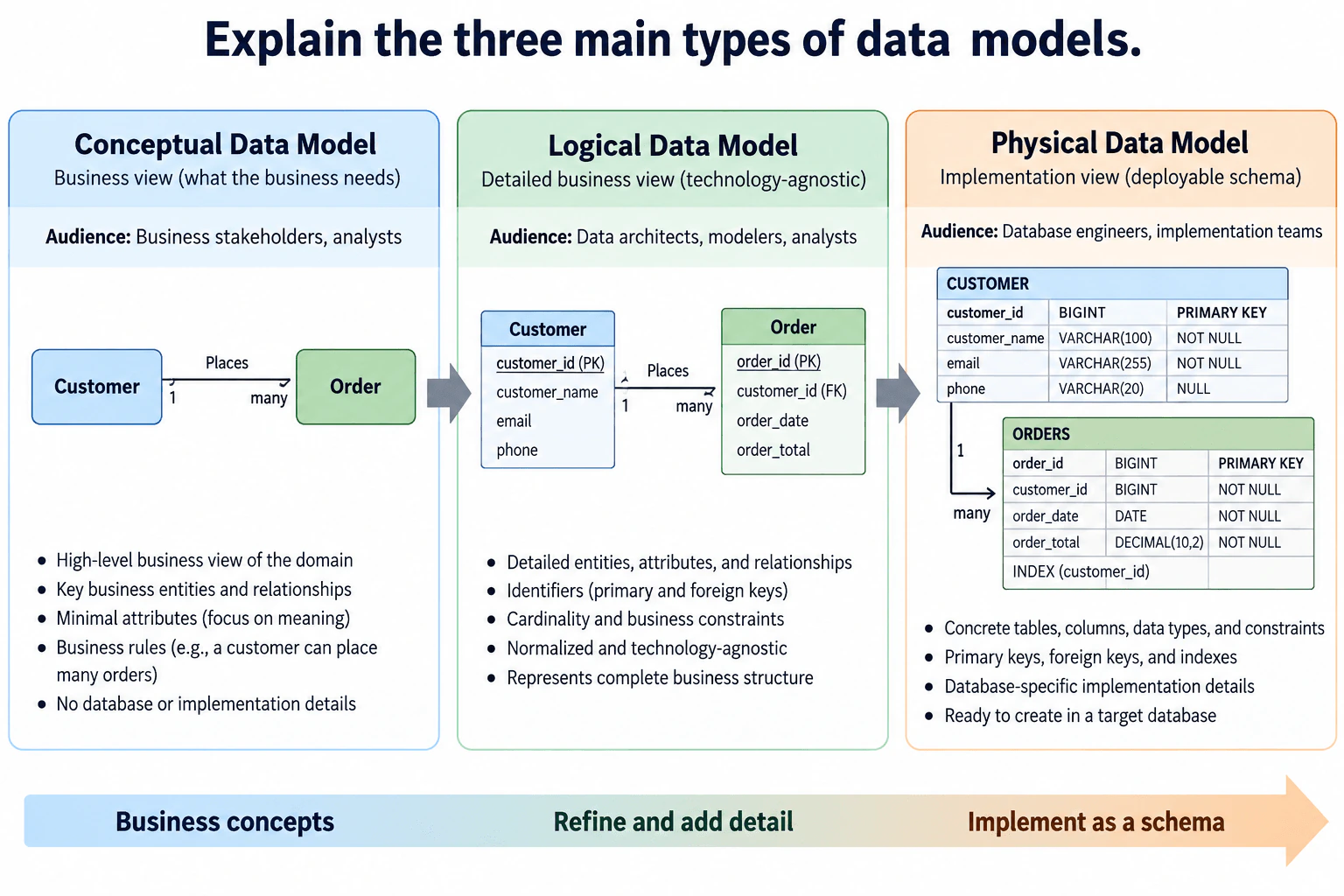
Explain the three main types of data models. diagram
How to Explain It in an Interview

A simple way to remember the progression is: business meaning → detailed structure → database implementation.

1. Conceptual Data Model

The conceptual model is the highest-level business view. Its main audience is business stakeholders and analysts. It focuses on the important business entities, their relationships, and high-level business rules without committing to database implementation details.

In the diagram, the main entities are Customer and Order. The relationship is that a Customer places Orders, with one customer able to place many orders. Attributes are kept minimal because the goal is to agree on the business meaning rather than design database tables. The constraints at this stage are mainly business rules, such as the one-to-many relationship between Customer and Order.

2. Logical Data Model

The logical model refines the conceptual design into a more detailed, technology-agnostic structure. Its audience commonly includes data architects, data modelers, and analysts.

The same Customer and Order concepts now have attributes and identifiers. Customer contains customer_id as its identifier plus customer_name, email, and phone. Order contains order_id as its identifier, customer_id as the reference back to Customer, order_date, and order_total. The one-to-many Customer-to-Order cardinality remains explicit.

At this stage, the model defines entities, attributes, identifiers, relationships, cardinality, and business constraints without choosing a specific database implementation. The diagram presents the logical structure as normalized and technology-agnostic, meaning the information is organized into related entities before database-specific storage details are introduced.

3. Physical Data Model

The physical model converts the logical design into an implementation-ready schema. Its audience is database engineers and implementation teams.

The conceptual Customer and Order entities become concrete CUSTOMER and ORDERS tables. The diagram assigns concrete column data types and nullability rules. CUSTOMER has customer_id BIGINT as the primary key, customer_name VARCHAR(100) NOT NULL, email VARCHAR(255) NOT NULL, and phone VARCHAR(20) NULL. ORDERS has order_id BIGINT as the primary key, customer_id BIGINT NOT NULL, order_date DATE NOT NULL, and order_total DECIMAL(10,2) NOT NULL.

The one-to-many relationship is implemented through ORDERS.customer_id referencing the customer side of the relationship. The physical design also shows an index on ORDERS.customer_id. That is a database implementation choice that can support access paths using customer_id, but it should not be described as automatically improving every workload.

How the Design Moves from Business Concepts to a Deployable Schema
  1. Start with business concepts: Customer places many Orders.
  2. Refine those concepts into entities with attributes, identifiers, relationships, cardinality, and business constraints.
  3. Keep that logical design independent of a specific database implementation.
  4. Map the logical entities to physical CUSTOMER and ORDERS tables.
  5. Choose concrete column data types, primary keys, nullability, relationship implementation, indexes, and other target-database details.

The key distinction is the amount of implementation detail. The conceptual model answers what the business cares about. The logical model answers how the information is structured. The physical model answers how that structure will actually be implemented in a database.

A useful tradeoff to mention is timing. If database-specific decisions are introduced too early, the design can become tied to a technology before the business structure is agreed upon. The physical stage is where those concrete implementation choices belong because a deployable schema requires them.

Technical Approach
  1. Identify the important business entities and relationships for the conceptual model.
  2. Add attributes, identifiers, cardinality, and business constraints to create the logical model.
  3. Keep the logical structure technology-agnostic.
  4. Map logical entities to physical tables and attributes to columns.
  5. Choose concrete data types, primary keys, nullability, relationship implementation, indexes, and other database-specific details.
  6. Verify that the physical schema still preserves the business meaning and relationships defined in the earlier models.
Practical Insights

There is no algorithmic time or memory complexity for this question. The main costs are design, change, and maintenance costs. Conceptual models are relatively easy to change because they contain little technical detail. Logical models require more care because attributes, identifiers, relationships, cardinality, and constraints must stay consistent. Physical models have the greatest operational impact because changes can affect deployed tables, constraints, indexes, migrations, storage, dependent applications, and database performance.

Why Interviewers Ask This

Interviewers want to know whether you understand how a data design progresses from business requirements to a detailed technology-neutral structure and then to an implementation-ready database schema. They also evaluate whether you can correctly distinguish the audience, entities, relationships, attributes, constraints, and implementation detail that belong at each modeling level.

Common interview mistakes

Common mistakes include treating conceptual, logical, and physical models as three unrelated designs instead of increasing levels of detail for the same design; adding database-specific data types or indexes to the conceptual model; assuming a logical model must already be tied to one DBMS; forgetting attributes, identifiers, relationships, cardinality, or constraints in the logical model; confusing business rules with implementation details; and describing the physical model as only tables while ignoring data types, keys, nullability, indexes, and other database-specific choices. Another mistake is claiming that an index such as ORDERS.customer_id always improves performance without considering the actual workload.

Interview tip

Use the phrase business meaning → detailed structure → database implementation. Then walk through one consistent example such as Customer and Order so the interviewer can see how the same one-to-many relationship becomes more detailed at each stage.
Interviewer may ask next
What is the main difference between a logical data model and a physical data model?

A logical data model defines the detailed structure of the information without committing to a particular database implementation. It includes entities, attributes, identifiers, relationships, cardinality, and business constraints. A physical data model maps that structure to concrete tables and columns with data types, primary keys, nullability, relationship implementation, indexes, and other database-specific choices.

Can the physical model differ from the logical model for performance or operational reasons?

Yes. The physical model can add database-specific implementation choices such as indexes or other storage structures to meet operational needs. Those choices should still preserve the business meaning and relationships established by the conceptual and logical models. Performance-related changes should be justified by the target database and workload rather than assumed to be universally faster.

2. Compare normalization and denormalization, including first, second, and third normal form.Data ModelingEasyAmazon

Question Details

Compare normalized and denormalized relational designs for transactional and analytical use. Define the dependency rule enforced by 1NF, 2NF, and 3NF, the anomalies each step addresses, and the read, write, storage, and maintenance effects of intentional duplication.

Short Interview Answer (30-60 seconds)

Normalize transactional data to reduce redundancy and anomalies: 1NF removes repeating groups, 2NF removes partial dependencies on a composite key, and 3NF removes transitive dependencies. Denormalize selectively for read-heavy analytics when fewer joins justify extra storage and coordinated maintenance of duplicated values.

Detailed Explanation

The practical choice depends on how the data will be used. If records change often, keeping each piece of information in one main place makes changes safer and reduces repeated values. If the system mostly reads and summarizes information, repeating some values can make common reads simpler. The important point is not to remove or add repetition blindly. First identify what each row represents, which values belong together, and which values depend on other values. Then choose the design that best balances safe changes, simple reads, storage, and ongoing upkeep.

Useful Questions to Ask the Interviewer
  1. Is the design mainly for transactional writes, analytical reads, or a mixture of both?
  2. Should I use a composite-key example to demonstrate the 2NF dependency rule explicitly?
  3. Should denormalization be discussed only as a modeling choice, or should I also explain how measurements would justify it?
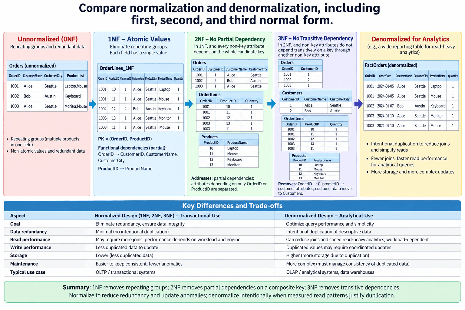
Compare normalization and denormalization, including first, second, and third normal form. diagram
How to Explain It in an Interview

Start with the practical decision: normalize when reducing duplication, maintaining integrity, and avoiding update anomalies are the priority, especially in transactional systems. Denormalize intentionally when a read-heavy analytical workload benefits from fewer joins and the extra storage and maintenance cost is acceptable.

In the diagram, the unnormalized Orders table contains a ProductList field with values such as multiple products in one cell. That is a repeating group and the field is not atomic.

1NF, or First Normal Form, removes repeating groups so each field contains one value. The diagram converts the data into OrderLines_1NF, where each row represents one order-product combination. Its composite primary key is (OrderID, ProductID). The important dependencies are visible: OrderID determines CustomerID, CustomerName, and CustomerCity, while ProductID determines ProductName. This removes the repeating-group problem, but redundancy can still remain.

2NF, or Second Normal Form, requires 1NF and removes partial dependencies. For a composite candidate key, every non-key attribute should depend on the whole key, not only one part of it. In OrderLines_1NF, the customer attributes depend only on OrderID, and ProductName depends only on ProductID. The diagram separates these into Orders, OrderItems, and Products. OrderItems keeps OrderID, ProductID, and Quantity because Quantity describes the specific order-product combination. This reduces duplication caused by partial dependencies and therefore reduces related insert, update, and delete anomalies.

3NF, or Third Normal Form, requires 2NF and removes transitive dependencies of non-key attributes through other non-key attributes. In the 2NF example, OrderID determines CustomerID, and CustomerID determines CustomerName and CustomerCity. Keeping customer attributes in Orders would repeat the same customer information across multiple orders. The 3NF design therefore separates Customers from Orders. The final normalized model shown in the diagram has Orders(OrderID, CustomerID), Customers(CustomerID, CustomerName, CustomerCity), OrderItems(OrderID, ProductID, Quantity), and Products(ProductID, ProductName). This reduces update anomalies because customer information has one primary location to maintain.

The normalized design is well suited to transactional use because duplicated descriptive data is minimized. A customer name or city can be changed in Customers instead of being changed in every order row. Maintenance and consistency are usually easier, but retrieving a complete business view may require joins across Orders, Customers, OrderItems, and Products. More joins do not automatically mean poor performance; actual performance depends on the workload, database engine, indexes, data size, and query plan.

Denormalization intentionally duplicates selected data for a specific access pattern. The diagram shows a wide FactOrders-style analytical table with OrderID, OrderDate, CustomerName, CustomerCity, ProductName, and Quantity. Customer and product descriptions repeat across rows. This can reduce joins and simplify read-heavy analytical queries. However, duplicated values consume more storage, and changing a duplicated value may require coordinated updates or a controlled refresh process to avoid inconsistencies.

So the tradeoff is: normalized designs generally reduce redundancy, update anomalies, and maintenance risk, while denormalized designs can simplify and sometimes speed read-heavy analytical access by accepting intentional duplication. Denormalization should be driven by measured read patterns rather than by an assumption that fewer joins are always faster.

Technical Approach
  1. Identify the grain of the current table and its candidate or primary key.
  2. Apply 1NF by removing repeating groups and making each field contain one value.
  3. If the key is composite, identify non-key attributes that depend on only part of that key and separate them to reach 2NF.
  4. Identify non-key attributes that depend on other non-key attributes and separate those transitive dependencies to reach 3NF.
  5. For transactional workloads, prefer the normalized model when integrity and safe updates dominate.
  6. For read-heavy analytics, consider intentional duplication only when measured access patterns justify fewer joins.
  7. Account for extra storage, consistency work, and maintenance when denormalizing.
Practical Insights

This is mainly a data and maintenance tradeoff, not an algorithmic Big-O problem. Normalization stores less repeated descriptive data and usually reduces the number of places that must change when a value is updated. Reads may require more joins. Denormalization stores repeated values, so storage increases and changes may require coordinated updates or refresh logic. In return, some analytical reads can use fewer joins. Actual query speed is workload-dependent and should be measured rather than assumed.

Why Interviewers Ask This

Interviewers want to see whether you understand the dependency rules behind 1NF, 2NF, and 3NF and can apply them to a realistic relational model. They also want judgment about when normalized transactional designs are preferable and when intentional duplication may be justified for analytical reads, including the effects on anomalies, reads, writes, storage, integrity, and maintenance.

Common interview mistakes

Common mistakes include saying that 1NF simply means 'no duplicate rows' instead of removing repeating groups and using atomic values; describing 2NF without mentioning partial dependency on a composite candidate key; confusing partial and transitive dependencies; forgetting that a relation with no composite candidate key cannot have the classic partial-dependency problem; claiming normalization always makes reads slow; claiming denormalization is always faster; calling every wide denormalized table a star schema; and ignoring the storage, update, consistency, and maintenance cost of duplicated values.

Interview tip

Use one dependency chain from the diagram. Say: 1NF removes repeating groups, 2NF removes attributes that depend on only part of the composite key, and 3NF removes attributes that depend on the key through another non-key attribute. Then connect the theory to the practical decision: normalize for integrity and safer updates; denormalize selectively for measured read-heavy needs.

Interviewer may ask next
When does 2NF matter if a table has a single-column candidate key?

The classic 2NF problem requires a composite candidate key because a partial dependency means a non-key attribute depends on a proper subset of that key. A single-column key has no non-empty proper subset, so a relation already in 1NF cannot have that form of partial dependency. You would still check for transitive dependencies when evaluating 3NF.

When would you intentionally denormalize the 3NF design shown here?

I would denormalize when a read-heavy analytical workload repeatedly needs the same customer, product, and order information together and measurements show that a wider representation provides a useful benefit. I would define how duplicated values are refreshed or updated, monitor consistency, and accept the extra storage and maintenance cost. I would not denormalize simply because the normalized design requires joins.

3. How would you choose a partition key for a fact table queried by both date and customer?Data ModelingMediumAmazon

Question Details

Evaluate access paths that filter by time, customer, or both. State assumptions about volume, customer skew, retention, pruning, clustering or sort keys, and whether a composite, derived, or two-level strategy avoids tiny partitions and hot keys.

Short Interview Answer (30-60 seconds)

Use coarse date partitions, such as daily or monthly, and cluster or sort by customer_id inside each partition. Avoid customer-only or date-plus-customer physical partitions that create too many partitions. For severe skew, add a small row-level salt or bucket that can split a hot customer's rows.

Detailed Explanation

The table contains a very large number of event or transaction rows and grows mostly by adding new rows. People need to find records by time, by customer, or by both. Some customers may generate much more activity than others, and the data may be kept for several years. The goal is to organize the stored rows so common searches avoid reading unnecessary data without creating huge numbers of tiny storage groups. The design must also keep unusually active customers from concentrating too much data in one place.

Useful Questions to Ask the Interviewer
  1. What percentage of queries filter by date only, customer only, or both?
  2. What is the daily or monthly data volume, and how many years of history are retained?
  3. How skewed is customer activity? Can one customer produce a large share of the rows?
  4. Which warehouse or storage engine is used, and does it support partition pruning, clustering, sorting, or file/block statistics?
  5. What partition or file sizes work well for that engine?
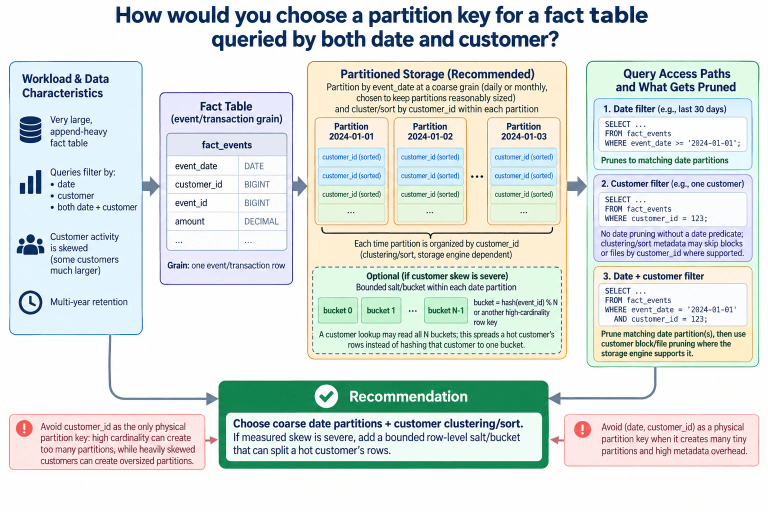
How would you choose a partition key for a fact table queried by both date and customer? diagram
How to Explain It in an Interview

I would start from the access paths rather than automatically choosing a composite physical partition key. The fact table has event or transaction grain: one row represents one event or transaction. The important columns in the diagram are event_date, customer_id, event_id, and a measure such as amount.

My default design is to physically partition by event_date at a coarse grain, usually daily or monthly depending on volume. The grain should be chosen so partitions remain reasonably sized. A date predicate can then prune date partitions outside the requested time range. This also fits multi-year retention because older time partitions can be managed along the same time boundary.

Inside each date partition, I would cluster or sort by customer_id when the storage engine supports that feature. Clustering or sorting is not the same thing as physical partitioning. It organizes data within the date partition so customer predicates may allow the engine to skip blocks or files using metadata supported by that engine.

For a date-only query, the engine can prune date partitions outside the requested range. For a customer-only query with no date predicate, there is no date partition pruning, so the query may need to consider all retained date partitions. Customer clustering, sorting, or file/block statistics may still reduce the amount of data read where supported. For a query containing both event_date and customer_id, the engine first narrows the read to the matching date partition or partitions, then may use customer-oriented block or file pruning inside those partitions.

I would avoid using customer_id as the only physical partition key. Customer identifiers usually have high cardinality, so this can create too many partitions. Customer activity can also be skewed, leaving a few heavily used customers with oversized partitions while many other customers create small ones.

I would also avoid physically partitioning by the pair (event_date, customer_id) when that combination creates many tiny partitions and high metadata overhead. A query can filter on both columns without requiring both columns to be physical partition keys.

If measured customer skew is severe, I would consider a bounded two-level strategy inside each date partition. Add a derived row-level salt or bucket such as bucket = hash(event_id) % N, or use another high-cardinality row key. This is different from hashing customer_id. If I hash only customer_id, every row for one hot customer still maps to one bucket. Hashing a row-level key can split that customer's rows across several buckets.

The tradeoff is that a lookup for one customer may have to read all N buckets for each relevant date partition because the bucket is derived from event_id rather than customer_id. Therefore, N should stay small and should be introduced only when measured skew justifies the extra complexity.

So my recommendation is: use coarse event_date partitions, cluster or sort by customer_id inside them where supported, and add a bounded row-level salt or bucket only for severe measured skew. I would validate the final choice using actual partition sizes, scan volume, pruning behavior, customer distribution, metadata overhead, and representative date-only, customer-only, and combined queries.

Technical Approach
  1. Measure the three main access paths: date-only, customer-only, and date-plus-customer queries.
  2. Measure fact-table volume, retention, customer cardinality, and customer skew.
  3. Choose a coarse event_date partition grain, such as day or month, that keeps partitions reasonably sized.
  4. Cluster or sort by customer_id inside each date partition where the engine supports it.
  5. Verify that date predicates prune partitions and that customer organization reduces block or file reads where supported.
  6. Avoid customer-only partitioning if cardinality creates too many partitions.
  7. Avoid physical (event_date, customer_id) partitioning if it creates many tiny partitions or excessive metadata.
  8. If severe skew remains, test a bounded derived row-level bucket such as hash(event_id) % N.
  9. Compare scan volume, partition size, skew, metadata cost, and maintenance complexity before finalizing the design.
Practical Insights

The main cost is the amount of data scanned and the number of physical partitions or files the engine must manage. Date-filtered queries can be much cheaper because irrelevant date partitions can be skipped. Customer-only queries cannot prune dates without a date predicate, although sorting, clustering, or file/block statistics may reduce reads where supported. Too many fine-grained partitions increase metadata and maintenance work. A bounded row-level bucket adds query and storage complexity, and a customer lookup may need to read all N buckets, but it can spread one very active customer's rows instead of concentrating them in one bucket.

Why Interviewers Ask This

This tests whether the candidate can turn real query patterns into a practical physical data layout. The interviewer wants to see judgment about date pruning, customer filtering, high-cardinality keys, customer skew, retention, partition size, metadata overhead, clustering or sorting, and when a composite or two-level strategy becomes harmful or useful.

Common interview mistakes

A common mistake is partitioning only by customer_id because it appears ideal for customer lookups. High cardinality can create too many physical partitions, and skew can leave some partitions much larger than others. Another mistake is using (event_date, customer_id) as a physical partition key without checking partition counts, which can produce many tiny partitions and high metadata overhead. A third mistake is treating clustering or sorting as identical to partition pruning. Date partition pruning removes whole date partitions, while clustering, sorting, or metadata may only allow block or file skipping where supported. Finally, hashing only customer_id does not split one hot customer's rows because all rows for that customer still hash to the same bucket.

Interview tip

Lead with the workload-driven choice: coarse date partitioning plus customer clustering or sorting. Then walk through date-only, customer-only, and combined filters. Explicitly discuss retention, partition size, customer skew, tiny partitions, and why a row-level bounded salt is different from hashing customer_id. Present the design as something you would validate with measured scan and partition statistics.

Interviewer may ask next
What would you do if one customer generates a very large percentage of all events?

I would first confirm that the skew is causing oversized partitions, concentrated scans, or processing imbalance. If it is, I would keep the coarse event_date partition and add a small bounded row-level bucket inside each date partition, such as hash(event_id) % N. That can distribute one hot customer's individual rows across several buckets. I would not hash only customer_id because every row for that customer would still map to the same bucket. The tradeoff is that a customer lookup may need to read all N buckets for the relevant date range, so N should remain small and be justified by measurements.

Why not physically partition directly by both event_date and customer_id?

That can work only when the resulting partition count and partition sizes are healthy for the storage engine. With many customers, a physical (event_date, customer_id) layout can create a very large number of tiny partitions and high metadata overhead. A safer default is coarse event_date partitioning with customer_id clustering or sorting inside each date partition. This preserves strong date pruning while still allowing customer-oriented block or file skipping where the engine supports it.

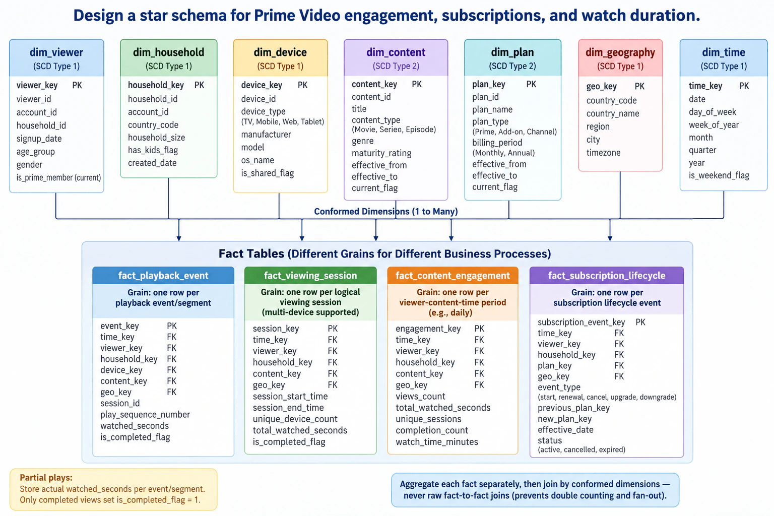
4. Design a star schema for Prime Video engagement, subscriptions, and watch duration.NEWData ModelingHardAmazon

Question Details

Declare grains for playback events, viewing sessions, content engagement, and subscription lifecycle facts. Define viewer, household, device, content, plan, geography, and time dimensions; handle multi-device sessions, partial plays, entitlement changes, changing metadata, and watch-time or retention measures without double counting.

Short Interview Answer (30-60 seconds)

I would model four separate facts for playback events, logical sessions, periodic content engagement, and subscription lifecycle events. They share conformed dimensions where appropriate. I would store actual watched seconds, preserve content and plan history with SCD Type 2, and aggregate facts separately before combining metrics.

Detailed Explanation

Prime Video needs to answer several related questions without counting the same activity twice. We need to know what a person watched, how long they watched, which actions belong to one viewing period, how interest in a title changes over time, and when access to a subscription starts or changes. The safest design keeps these activities in separate tables because they happen at different levels of detail. Shared descriptive information connects them consistently, so reports can combine viewing, subscription, location, device, and calendar information without repeating totals.

Useful Questions to Ask the Interviewer
  1. Should content engagement be summarized daily, or should another reporting period be used?
  2. What business rule defines when one logical viewing session starts and ends, especially when activity moves across devices?
  3. Should retention be measured at viewer, household, or subscription-plan level?
  4. Do entitlement changes need full point-in-time history, or is lifecycle-event history sufficient?
  5. Which content and plan attributes must preserve their historical values when they change?
Design a star schema for Prime Video engagement, subscriptions, and watch duration. diagram
How to Explain It in an Interview

I would start by declaring four fact-table grains because the four business processes should not be mixed into one fact.

  1. fact_playback_event: one row per playback event or segment. event_key is the primary key. The fact contains foreign keys time_key, viewer_key, household_key, device_key, content_key, and geo_key. It also stores session_id, play_sequence_number, watched_seconds, and is_completed_flag. This is the detailed source for partial-play behavior. A partial play contributes only its actual watched_seconds; it is not treated as a full play. The diagram's rule is that only completed views set is_completed_flag = 1.
  1. fact_viewing_session: one row per logical viewing session. session_key is the primary key. It contains time_key, viewer_key, household_key, content_key, and geo_key, plus session_start_time, session_end_time, unique_device_count, total_watched_seconds, and is_completed_flag. The grain is a logical session, not a device connection. That lets one session represent activity involving multiple devices while unique_device_count records how many distinct devices participated.
  1. fact_content_engagement: one row per viewer-content-time period, for example one day. engagement_key is the primary key. It contains time_key, viewer_key, household_key, content_key, and geo_key. Its measures are views_count, total_watched_seconds, unique_sessions, completion_count, and watch_time_minutes. watch_time_minutes is a representation derived from watched time; it must not be added again to total_watched_seconds as though it were a separate measure.
  1. fact_subscription_lifecycle: one row per subscription lifecycle event. subscription_event_key is the primary key. It contains time_key, viewer_key, household_key, plan_key, and geo_key. It records event_type such as start, renewal, cancellation, upgrade, or downgrade, together with previous_plan_key, new_plan_key, effective_date, and status. These event rows preserve entitlement changes instead of simply overwriting the current subscription state.

The dimensions are shared descriptive entities. dim_viewer, dim_household, dim_device, dim_geography, and dim_time are shown as SCD Type 1 dimensions in the diagram. Type 1 means tracked changes replace the prior descriptive value. dim_content and dim_plan are SCD Type 2 dimensions. They contain effective_from, effective_to, and current_flag, so an important metadata change creates a new surrogate-key row while earlier fact rows continue to reference the historical version.

dim_viewer uses viewer_key and includes viewer, account, household, signup, demographic, and current Prime-member attributes. dim_household uses household_key and describes the household. dim_device uses device_key and describes device type, manufacturer, model, operating system, and whether it is shared. dim_content uses content_key and describes title, content type, genre, and maturity rating. dim_plan uses plan_key and describes plan name, plan type, and billing period. dim_geography uses geo_key and contains country, region, city, and time zone. dim_time uses time_key and provides date, day-of-week, week, month, quarter, year, and weekend attributes.

The dimensions are conformed: the same viewer, household, content, geography, and time meanings can be reused across the applicable facts rather than creating incompatible copies. Device applies directly to the playback-event fact in the diagram, while plan applies directly to the subscription-lifecycle fact.

The key rule for watch time and retention is to respect grain. I would not join raw playback rows directly to raw session, engagement, or subscription rows and then sum measures. A many-row fact joined to another many-row fact can create fan-out, multiplying rows and inflating totals. Instead, aggregate each fact independently to the requested reporting grain, then combine the aggregated results through conformed dimensions.

For watch duration, actual watched_seconds is captured at the playback level and summarized into session or engagement measures at their declared grains. For retention, derive subscription state or lifecycle outcomes from fact_subscription_lifecycle at the requested viewer, household, plan, and time grain. If retention analysis also needs viewing behavior, first aggregate engagement or session measures to that same analytical grain, then combine the already-aggregated results. This keeps entitlement history and watch-time totals consistent without double counting.

Technical Approach
  1. Identify the four business processes: playback events, logical viewing sessions, periodic content engagement, and subscription lifecycle events.
  2. Declare one row-level grain for each fact before selecting measures.
  3. Use conformed viewer, household, content, geography, and time dimensions where applicable; use device for playback and plan for subscription lifecycle.
  4. Store actual watched_seconds at playback grain so partial plays remain accurate.
  5. Roll playback activity into logical sessions and record unique_device_count for multi-device behavior.
  6. Produce viewer-content-period engagement measures such as views, watched seconds, unique sessions, and completions.
  7. Record subscription starts, renewals, cancellations, upgrades, and downgrades as lifecycle events with effective dates.
  8. Preserve changing content and plan metadata using the SCD Type 2 effective-date structure shown in the diagram.
  9. Aggregate each fact independently to the required analytical grain.
  10. Combine only those aggregated results through conformed dimensions to avoid fact-to-fact fan-out and double counting.
Practical Insights

The playback-event fact will usually contain the most rows because it stores the finest viewing detail. Session and engagement facts reduce repeated reporting work by storing summaries at coarser grains. Subscription lifecycle history requires additional event rows as plans change. SCD Type 2 content and plan dimensions also grow when tracked metadata changes. The main maintenance cost is assigning facts to the correct dimension version and keeping rollups consistent. The main query risk is joining detailed fact tables directly; aggregating each fact to the needed reporting level first reduces both processing work and accidental duplication.

Why Interviewers Ask This

This question tests whether a Data Engineer can declare correct fact grains, separate different business processes, choose appropriate dimensions and measures, preserve historical metadata, represent subscription and entitlement changes, support multi-device viewing, and calculate watch-time or retention metrics without double counting.

Common interview mistakes

Common mistakes include putting all four business processes into one fact table, mixing playback and session grain, storing only completed plays and losing partial watch time, treating one device connection as the required logical session, overwriting changing content or plan metadata that should retain history, representing upgrades or downgrades only as a current plan value, adding watch_time_minutes and total_watched_seconds as though they were independent measures, joining raw fact tables directly and creating fan-out, and calculating retention at a grain inconsistent with the subscription lifecycle data.

Interview tip

Lead with the four fact grains. Then map the applicable conformed dimensions, explain partial plays and multi-device sessions, describe SCD Type 2 history for content and plan, and finish with the anti-double-counting rule: aggregate each fact independently before combining metrics.

Interviewer may ask next
How would you calculate watch time by subscription plan without double counting?

First aggregate watch time from the session or engagement fact to the required viewer and reporting-period grain. Separately derive the applicable plan or subscription outcome from fact_subscription_lifecycle for that same viewer and period. Then combine those already-aggregated results using the shared viewer and time context. Do not join raw playback events directly to raw lifecycle events because multiple playback rows and multiple subscription events can multiply each other and inflate watch time.

How would you handle content or plan metadata that changes over time?

Use the SCD Type 2 structure shown for dim_content and dim_plan. When a tracked attribute changes, create a new surrogate-key row with a new effective period instead of overwriting the historical row. Keep effective_from, effective_to, and current_flag on the dimension version. Historical facts continue to reference the version that applied when the fact was recorded, while current reporting can use the row marked as current.

5. Explain the extraction, transformation, and loading steps of an ETL process.Data PipelinesEasyAmazon

Question Details

Describe how source data is acquired, validated, converted, joined or aggregated, and committed to the destination. Include staging, checkpoints, metadata, rejected records, and the point at which downstream consumers can safely read a completed load.

Short Interview Answer (30-60 seconds)

ETL moves data from source systems into a trusted destination. First, I extract files, tables, or API data into staging and validate it, sending invalid records to quarantine. Next, I clean, convert, join, or aggregate the accepted data. Finally, I write and commit the result to the destination. Downstream consumers read only after that commit succeeds. Checkpoints and load metadata track progress and status. The trade-off is that stronger validation adds processing time but reduces the risk of publishing bad data.

Detailed Explanation

An ETL process is a controlled way to move information from where it starts to where people can safely use it. First, the source information is copied into a temporary holding area. It is checked before continuing, and unacceptable records are separated instead of being mixed with good records. The accepted information is then cleaned, converted, combined, or summarized as needed. Finally, the finished result is written to its destination. Only after that final write is successfully committed should reports or other users rely on it. Progress and basic facts about each load are also recorded along the way.

Useful Questions to Ask the Interviewer
  1. Should I explain ETL as a general batch process, or is there a specific source or destination you want me to assume?
  2. Should invalid records stop the entire load, or should valid records continue while rejected records are quarantined?
  3. What publication or commit behavior should downstream consumers rely on before they read the result?
Explain the extraction, transformation, and loading steps of an ETL process. diagram
How to Explain It in an Interview
1. Extract source data

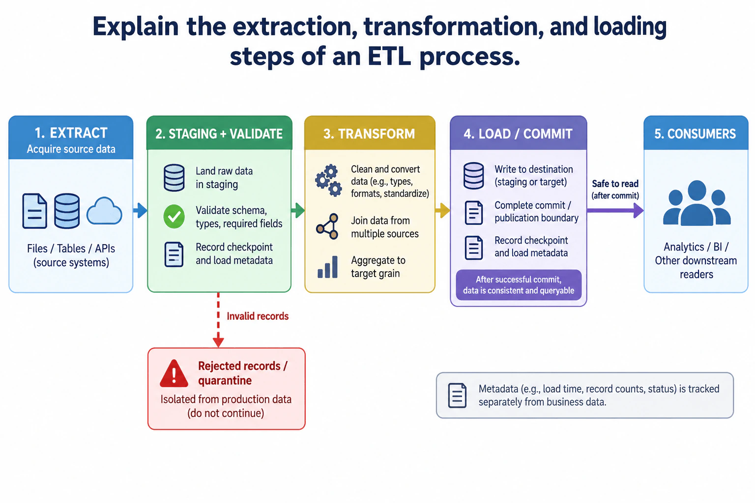
I would start by saying that extraction acquires data from the source systems without changing its business meaning. In this design, the sources are represented generically as files, tables, or APIs. The extracted records move from the source boundary into staging. Staging gives the pipeline a controlled place to hold the raw input before transformation. I would not invent a schedule, streaming system, change-data-capture method, or vendor because none is shown in the diagram.

2. Stage and validate the input

Next, I land the raw data in staging and validate its basic contract. The diagram specifically shows checks for schema, data types, and required fields. Accepted records continue to transformation. Invalid records take a separate failure path into the rejected-records or quarantine area and do not continue into production data. I also record a checkpoint and load metadata at this stage. The checkpoint records processing progress, while metadata records facts about the load rather than carrying the business records themselves.

3. Transform the accepted data

The transformation stage prepares the accepted records for the destination. I clean and standardize values, convert data types or formats, join data from multiple sources when required, and aggregate records to the target grain when required. The important point is that transformation changes the representation or structure needed by the destination while preserving the intended business meaning. I would not invent join keys, schemas, partition keys, or aggregation rules because the question and diagram do not define them.

4. Load and commit the result

After transformation, I write the resulting data to the destination. The diagram shows a Load / Commit boundary, so I would distinguish writing data from successfully publishing it. I also record a checkpoint and load metadata for this stage. A load should not be described as complete merely because processing ran; the final commit or publication boundary must succeed. This prevents downstream users from being told that data is ready while the destination may still contain incomplete output.

5. Publish only after the successful commit

The key correctness rule in this design is consumer visibility. Analytics, BI, and other downstream readers should treat the result as safe to read only after the successful commit. Before that boundary, data may still be in staging or in the middle of the load. The diagram therefore separates writing output from the point at which the completed result becomes available to consumers. The exact atomicity scope depends on the destination technology, so I would not claim a universal table-level or transaction-level guarantee that is not shown.

6. Track rejected records, checkpoints, and metadata separately

Finally, I would explain the supporting controls. Rejected records are isolated in quarantine instead of silently disappearing or entering production data. Checkpoints record progress so the pipeline can identify how far processing reached, although the exact retry or recovery behavior is not specified in this design. Load metadata, such as load time, record counts, and status, is tracked separately from business data. Together, these controls make the ETL process easier to validate and operate without confusing operational state with the actual dataset.

Technical Approach
  1. Acquire source data from the shown files, tables, or APIs.
  2. Land the raw input in staging.
  3. Validate schema, data types, and required fields.
  4. Send invalid records to quarantine and stop those records from continuing.
  5. Record the staging checkpoint and load metadata.
  6. Clean and standardize accepted records, convert formats or types, join sources when needed, and aggregate to the required target grain.
  7. Write the transformed result to the destination.
  8. Record the load checkpoint and metadata.
  9. Complete the commit or publication boundary.
  10. Allow downstream consumers to read the completed load only after that commit succeeds.
Practical Insights

The main trade-off is correctness versus speed. The benefit is that staging and validation catch bad input before it reaches the destination. The downside is that every check and intermediate step adds processing time and storage work. The benefit of quarantining rejected records is that valid production data stays clean and failures remain visible. The downside is that rejected records need separate review or correction. Waiting for a successful commit before consumers access the data gives a clear publication boundary, but it may delay availability compared with exposing partial results early. We accept these costs because this ETL design values a completed, validated result over slightly faster but potentially inconsistent data.

Why Interviewers Ask This

Interviewers ask this question to see whether you understand the complete movement of data, not just the words extract, transform, and load. They want to know whether you can explain where validation belongs, how bad records are separated, how data is reshaped, and when a completed result becomes safe for downstream consumers to read. A strong answer also shows that you understand checkpoints and metadata as controls for tracking a reliable load.

Common interview mistakes

Common mistakes are describing ETL as only three verbs and ignoring the reliability boundaries around them. A candidate may skip staging, forget to validate schema and required fields, silently discard bad records instead of quarantining them, or confuse metadata with business data. Another mistake is saying data is ready as soon as a write starts rather than after the successful commit or publication boundary. It is also incorrect to invent exactly-once behavior, retry rules, join keys, schemas, partitioning, or vendor-specific guarantees that are not defined by the question or diagram.

Interview tip

Explain ETL as one end-to-end flow: acquire, stage and validate, transform, load and commit, then publish to consumers. Spend extra time on the two correctness boundaries interviewers often look for: invalid records go to quarantine, and downstream consumers read only after the completed load is successfully committed.

Interviewer may ask next
What would you do if the load fails after some destination data has already been written?

I would first prevent downstream consumers from treating that partial result as a completed load. The requirement that changes is recovery: the pipeline now has to distinguish partially written destination data from a successfully committed publication. The affected area is the Load / Commit stage and its checkpoint. I would use whatever commit or publication mechanism the destination actually supports so incomplete work remains unpublished or can be safely replaced. I would inspect the recorded checkpoint and load metadata to determine how far the run progressed, then validate the destination before declaring recovery complete. Rejected source records would remain in quarantine and would not be mixed into the recovery path. I would keep the original extraction, staging, validation, and transformation flow unchanged. I would not claim that simply rerunning is safe unless the destination supports a repeatable write strategy. The downside is additional recovery logic and potentially more staging storage, but the benefit is that consumers do not see an incomplete result.

How would you handle records that fail validation while allowing valid records to complete the ETL load?

I would keep the validation branch shown in the design: valid records continue, while invalid records are sent to the rejected-records or quarantine area and do not enter production data. The changed requirement is that one bad record should not necessarily block every valid record. The Stage + Validate component therefore classifies each input against the defined schema, type, and required-field rules. Accepted records move into Transform, while rejected records follow the separate quarantine path. I would record counts and status in load metadata so accepted and rejected volumes can be checked. The transformation, destination load, and final consumer publication boundary stay unchanged for accepted records. Corrected rejected records should only re-enter processing through a controlled future run if that behavior is defined; I would not silently push them forward. The main downside is operational work to investigate and correct quarantined records, but this approach prevents known bad data from contaminating the destination while preserving useful valid data.

6. Compare ETL and ELT and explain when each is appropriate.Data PipelinesEasyAmazon

Question Details

Compare where transformation runs, when raw data is retained, and how compute, governance, latency, schema control, and reprocessing differ between ETL and ELT. Relate the choice to a traditional warehouse, cloud warehouse, and data lake or lakehouse.

Short Interview Answer (30-60 seconds)

ETL transforms data before loading it into the destination, so it fits cases that need strong upfront schema control, filtering, or a traditional warehouse with limited compute. ELT loads raw or minimally processed data first and transforms it inside or near the target, which fits scalable cloud warehouses, data lakes, and lakehouses. ELT often makes reprocessing easier when raw data is retained, while ETL provides more control before data reaches the target.

Detailed Explanation

ETL and ELT are two ways to move and prepare information for analysis. The main difference is when the information is changed. With ETL, it is cleaned and organized before it reaches its final home. With ELT, the original or lightly changed information is stored first and organized afterward. The choice affects how quickly information arrives, how easily old information can be processed again, where computing work happens, how early rules are enforced, and whether the original information remains available for future needs.

Useful Questions to Ask the Interviewer
  1. Is the destination a traditional warehouse, a scalable cloud warehouse, or a data lake or lakehouse?
  2. Do we need to retain raw or minimally processed data for audits or future reprocessing?
  3. Must sensitive or invalid data be filtered before it is loaded into the destination?
  4. Is faster initial ingestion more important than having fully transformed data available immediately?
Compare ETL and ELT and explain when each is appropriate. diagram
How to Explain It in an Interview
1. Start with where transformation happens

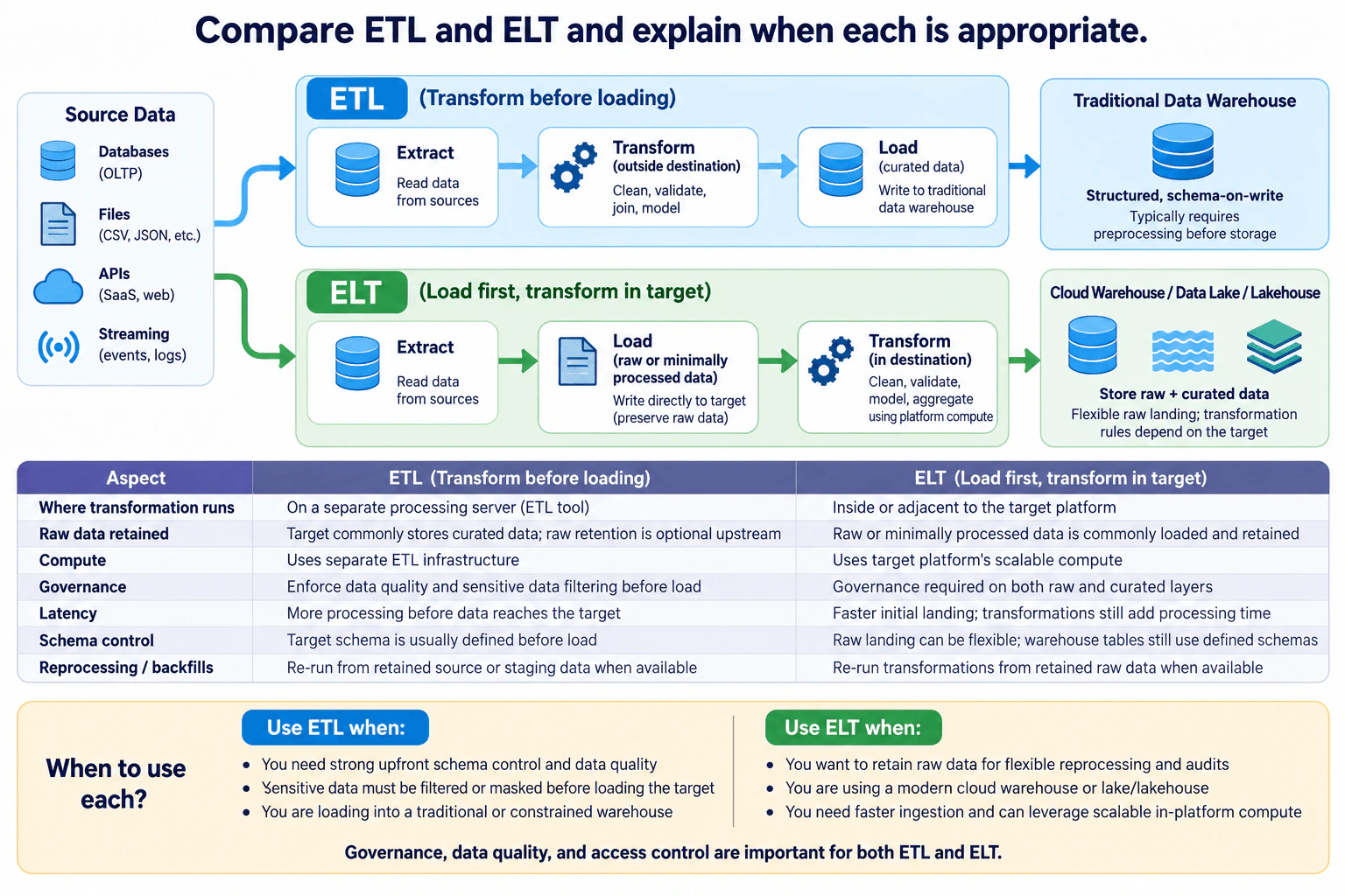
I would first explain that ETL means Extract, Transform, Load. Data is read from sources such as databases, files, APIs, or streams. It is transformed outside the destination and then loaded as curated data. ELT means Extract, Load, Transform. Data is read from the same kinds of sources, loaded first as raw or minimally processed data, and transformed inside or adjacent to the target platform. That transformation location is the fundamental design difference.

2. Compare raw-data retention and reprocessing

In ETL, the target commonly stores curated data. Raw retention is optional and may exist upstream or in staging, but it is not guaranteed by the ETL pattern itself. When retained source or staging data is available, ETL processing can be rerun from that data. In ELT, raw or minimally processed data is commonly loaded and retained. That makes it easier to rerun transformations for changed business rules, corrections, audits, or historical backfills when the retained raw data is available.

3. Compare compute and latency

ETL commonly uses separate processing infrastructure before the destination. This is useful when the destination is a traditional or constrained warehouse that should mainly receive prepared data. ELT uses the target platform's scalable compute for transformation. Its benefit is faster initial landing because transformation does not have to finish before the load. However, this does not guarantee lower end-to-end analytical latency. The later transformations still consume processing time before curated results are ready.

4. Compare schema control and governance

ETL usually defines the target schema before load and can enforce data-quality or sensitive-data rules during transformation. This provides strong control before data reaches the destination. ELT permits a more flexible raw landing, while curated warehouse tables can still use defined schemas. Governance matters in both patterns. In ELT, governance must cover raw and curated layers because the retained raw data may contain sensitive or poorly structured values. In ETL, governance also applies to the transformation layer before data is loaded.

5. Relate the choice to the destination

For a traditional data warehouse, ETL is often appropriate because data is prepared before loading and the warehouse may have limited transformation capacity. For a modern cloud warehouse, ELT is often attractive because the target can provide scalable in-platform compute. Data lakes and lakehouses also commonly support ELT-style workflows because raw data can be retained and transformed into curated forms later. These are common architectural tendencies rather than absolute rules. Compute, governance, latency, schema requirements, and retention needs should drive the decision.

6. Make the practical choice

I would choose ETL when strong preprocessing, schema control, data-quality checks, or sensitive-data filtering must happen before data is loaded into the target. I would also consider it for a traditional or constrained warehouse. I would choose ELT when I want faster initial ingestion, scalable target-side processing, and retained raw data for audits, changing requirements, or reprocessing. In both cases, governance, data quality, and access control remain important.

Technical Approach
  1. Identify whether the destination is a traditional warehouse, cloud warehouse, data lake, or lakehouse.
  2. Determine where transformation should run.
  3. Decide whether raw or minimally processed data must be retained.
  4. Compare separate processing compute with target-platform compute.
  5. Compare faster initial landing with the time required to produce curated data.
  6. Determine how much schema control and sensitive-data filtering must happen before loading.
  7. Determine what retained data will support future reprocessing or backfills.
  8. Choose ETL or ELT based on those constraints rather than assuming one pattern is always better.
Practical Insights

The benefit of ETL is strong control before data enters the destination. Data can be cleaned, validated, reshaped, or masked first, and a traditional warehouse receives prepared data. The downside is that this work happens before loading, so initial availability can be delayed. Reprocessing also depends on whether source or staging data was retained. The benefit of ELT is faster initial landing and easier reprocessing when raw data is retained. It can also use scalable target compute. The downside is that raw storage increases governance and access-control responsibilities, while later transformations still consume compute and time. We accept these trade-offs based on the destination, security needs, latency requirements, available compute, and expected need for historical reprocessing.

Why Interviewers Ask This

Interviewers use this question to test architectural judgment rather than memorization. A strong candidate should understand where transformation runs, how raw-data retention affects reprocessing, how destination compute influences the design, and how governance and schema control differ. The question also tests whether the candidate can relate ETL and ELT to traditional warehouses, cloud warehouses, data lakes, and lakehouses without treating either pattern as universally better.

Common interview mistakes

A common mistake is saying ETL always discards raw data. Raw data may still be retained upstream or in staging; ETL only defines transformation before the target load. Another mistake is saying ELT always means schema-on-read. Raw landing can be flexible, while curated warehouse tables can still enforce defined schemas. Candidates also sometimes say ELT is always faster end to end. It mainly allows faster initial landing; transformation still takes time. Another mistake is treating governance as an ETL-only concern. Both patterns require governance, data quality, and access control, and ELT may require controls across both raw and curated layers.

Interview tip

Start with the core distinction: ETL transforms before loading, while ELT loads first and transforms in or near the target. Then compare raw retention, compute location, latency, schema control, governance, and reprocessing. Finish with the practical choice: ETL often fits strict upfront controls and traditional or constrained warehouses; ELT often fits scalable cloud platforms and retained raw data. Avoid claiming that either approach is always better.

Interviewer may ask next
How would your choice change if the business frequently changes transformation rules and needs to rebuild several years of historical data?

I would lean more strongly toward ELT if raw or minimally processed historical data is retained and the target has enough compute for repeated transformations. The changed requirement is reprocessing flexibility. In the existing ELT flow, data is extracted, loaded first, and transformed afterward. Retained raw data therefore becomes the reusable input for rebuilding curated outputs when business rules change. Correctness still depends on applying the new transformation rules consistently and validating the resulting curated data before it is used. Governance and access control remain important because the retained raw layer may contain sensitive values. Reprocessing can start again from retained raw data when available instead of requiring a fresh extraction from every original source. The main downside is additional storage and target-compute cost, especially when several years of data are transformed repeatedly. The rest of the original ELT flow remains unchanged.

What if sensitive data is not allowed to enter the analytical destination until it has been masked or filtered?

I would favor ETL because the required control must happen before the destination receives the data. The affected part of the existing flow is the transformation step outside the destination. Data is extracted from the source, sensitive values are filtered or masked during transformation, and only the approved curated result is loaded into the traditional or constrained warehouse. This keeps the destination aligned with the requirement while preserving the same Extract, Transform, Load sequence shown in the diagram. Data-quality and schema rules can be applied in the same pre-load transformation boundary. If historical processing is needed later, the ETL flow can be rerun from retained source or staging data when that data is available. The main downside is that transformation must finish before loading, so initial data availability can take longer than with a load-first approach. The source and destination boundaries remain otherwise unchanged.

7. Design an ETL process that collects event data in real time.Data PipelinesMediumAmazon

Question Details

Start from an event producer and design ingestion, durable buffering, validation, transformation, storage, and serving for near-real-time consumers. State throughput and latency assumptions and cover partitioning, ordering, duplicates, late events, schema evolution, replay, and monitoring.

Short Interview Answer (30-60 seconds)

I would place a durable partitioned event buffer between producers and stream processing, then validate, deduplicate, handle late events, transform, and write clean records to serving storage. I would preserve ordering only within each stable-key partition and use idempotent writes so replay is safe. More partitions increase parallelism, but they also add coordination and do not provide global ordering.

Detailed Explanation

The goal is to collect activity as it happens, keep it safe when another part of the system is temporarily unavailable, check that each item is valid, remove repeated items, prepare it for analysis, and make the result available quickly. Related activity should stay in the correct sequence where that matters. Items that arrive late or have an unexpected shape must not silently disappear. The design must also let us read old activity again after a failure and show whether the system is keeping up with incoming work.

Useful Questions to Ask the Interviewer
  1. What peak number of events per second should the pipeline support?
  2. What end-to-end latency is acceptable for near-real-time consumers?
  3. Which field should be the stable entity key for partitioning and ordering?
  4. How late can an event arrive before it should go to correction or quarantine?
  5. How long must the durable event log retain data for replay?
Design an ETL process that collects event data in real time. diagram
How to Explain It in an Interview
1. Define the Event Producers and event contract

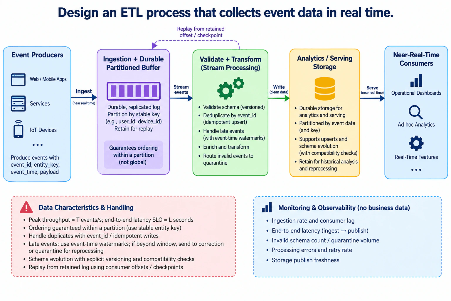
I would begin with the events themselves. The Event Producers in the diagram are web or mobile applications, services, and IoT devices. Each event carries event_id, entity_key, event_time, and payload. event_id identifies the logical event for duplicate handling. entity_key is the stable key used for partitioning. event_time is when the event occurred at the source. Producers continuously send these events to ingestion.

2. Use the Ingestion + Durable Partitioned Buffer

I would put a durable, replicated log between producers and processing instead of sending events directly to the transformation stage. The buffer is partitioned by a stable key such as user_id or device_id. This allows partitions to be processed in parallel while preserving ordering within one partition. I would explicitly state that this does not create global ordering across all partitions. The retained log also provides the source for replay. Until the interviewer gives real numbers, I would express capacity as peak throughput T events/s and end-to-end latency SLO L seconds.

3. Validate + Transform in stream processing

The Validate + Transform stage reads events from the durable buffer. It first validates the versioned schema. Invalid records go to quarantine rather than being silently accepted. It then deduplicates by event_id, enriches the event when needed, and transforms it into the destination shape. Repeated processing must not create repeated business results, so the processing and destination-write behavior must be idempotent. Schema evolution uses explicit versions and compatibility checks rather than assuming every producer change is safe.

4. Handle ordering, duplicates, and late events correctly

Ordering is guaranteed only within a partition, so related events must use the same stable entity key when order matters. Duplicate events are detected using event_id. For time-sensitive logic, I would use event_time, not merely the time when processing happens. Event-time watermarks define how long the processor accepts delayed records into normal processing. Events beyond that window go to correction or quarantine for reprocessing. A longer late-event window improves event-time completeness but requires more state and can delay final results.

5. Write to Analytics / Serving Storage

Clean data moves from stream processing into Analytics / Serving Storage. The diagram uses durable storage for both analytics and near-real-time serving. It is partitioned by event date and, when appropriate, another key. The storage supports upserts so replaying the same logical event can update the existing result instead of creating another copy. Schema evolution remains explicit and compatibility checked. Historical data is retained for analysis and reprocessing. Near-Real-Time Consumers such as operational dashboards, ad-hoc analytics, and real-time features read from this serving boundary.

6. Replay from retained offsets or checkpoints

If processing fails or historical data must be reprocessed, I would replay retained events from a chosen consumer offset or checkpoint. Replay sends previously retained data through the same validation and transformation path again. Deduplication by event_id and idempotent destination writes make repeated processing safe. Replay is different from accepting a permanently invalid record: schema-invalid data remains quarantined until it is corrected. Recovery is complete only when processing catches up and the destination is fresh again.

7. Monitor the pipeline separately from business data

Monitoring and Observability are not part of the main business-data path. I would monitor ingestion rate and consumer lag to see whether processing is keeping up, end-to-end latency from ingestion to publication, invalid-schema count and quarantine volume, processing errors and retry rate, and storage publication freshness. These signals tell operators whether the pipeline is receiving data, processing it correctly, recovering from failures, and delivering fresh output to consumers.

Technical Approach
  1. Define the event contract with event_id, entity_key, event_time, payload, and schema version.
  2. Ingest events into a durable replicated log partitioned by the stable entity key.
  3. Process partitions in parallel while preserving ordering only inside each partition.
  4. Validate the schema and quarantine invalid records.
  5. Deduplicate by event_id and handle late arrivals using event-time watermarks.
  6. Enrich and transform accepted events.
  7. Write clean records to Analytics / Serving Storage using idempotent upserts.
  8. Serve Near-Real-Time Consumers from that storage.
  9. Replay retained events from offsets or checkpoints when recovery or reprocessing is required.
  10. Monitor ingestion rate, lag, latency, invalid records, retries, errors, and publication freshness.
Practical Insights

The benefit is that partitioning lets multiple workers process independent event groups in parallel, so throughput can grow with useful partition count. The downside is that ordering exists only inside one partition, and additional partitions increase coordination overhead. Deduplication and late-event handling also require state, so longer retention or watermark windows increase memory or storage cost. The benefit of retaining the event log is that failures and corrections can be replayed safely. The downside is extra retained data and reprocessing work. Strong schema validation protects downstream quality, but quarantined records may delay some results. We accept these costs because the design favors correct, recoverable near-real-time data instead of minimizing operational work at the expense of correctness.

Why Interviewers Ask This

This question tests whether a candidate can design a reliable streaming data path instead of only naming components. The interviewer wants to see judgment around partitioning, ordering scope, duplicate handling, late events, schema changes, safe replay, and observable freshness. It also tests whether the candidate separates message delivery from correct business results and understands why durability, validation, idempotency, and recovery matter in production.

Common interview mistakes

Common mistakes include sending producers directly to the destination without a durable buffer, claiming global ordering when only partition-local ordering exists, using an unstable partition key, ignoring duplicate events, confusing event time with processing time, dropping late or schema-invalid records silently, assuming schema changes are automatically compatible, and replaying data without deduplication or idempotent writes. Another mistake is treating a processing success signal as proof that correct data reached consumers. Monitoring only uptime is also weak; the design should watch consumer lag, end-to-end latency, quarantine volume, errors, retry rate, and publication freshness.

Interview tip

Draw and explain the main flow first: Event Producers → Ingestion + Durable Partitioned Buffer → Validate + Transform → Analytics / Serving Storage → Near-Real-Time Consumers. Then explain the three main correctness decisions: ordering only within a stable-key partition, event_id-based duplicate handling with idempotent writes, and event-time handling for late events. Finish with replay and monitoring. Keep throughput as T events/s and latency as L seconds until the interviewer provides real requirements.

Interviewer may ask next
What would you change if event volume increased sharply while the latency target stayed the same?

I would keep the same architecture and increase parallelism around the durable partitioned buffer and stream-processing stage. The changed requirement is higher peak throughput T events/s while preserving the same end-to-end latency target L. I would first inspect ingestion rate, consumer lag, processing latency, and destination freshness to identify the bottleneck.

If processing capacity is limiting throughput, I would increase useful partition count and matching processing parallelism. Events for the same stable entity_key must still be routed consistently so their ordering remains inside one partition. I would not claim that adding partitions creates global ordering.

Validation, event_id deduplication, watermark handling, quarantine, compatibility checks, and idempotent destination writes remain unchanged. Replay still begins from retained offsets or checkpoints. The main downside is additional partition coordination and greater pressure on processing and storage. I would scale only after measuring which boundary is limiting throughput, because adding processing capacity cannot help if the durable buffer or destination write path is already saturated.

How would you handle events that arrive very late or are replayed after the destination already contains their earlier result?

I would keep the same pipeline and treat late arrival and replay as correctness cases. For delayed events, event_time determines lateness. If the event is still within the accepted watermark window, processing can handle it normally and update the result when needed. If it is beyond that window, the diagram's design sends it to correction or quarantine for controlled reprocessing rather than silently dropping it.

For replay, the processor rereads retained events from a selected offset or checkpoint. Schema validation runs again, event_id is reused for duplicate handling, and the destination performs an idempotent upsert so the same logical event does not create another business result. An incompatible record remains isolated in quarantine until corrected.

Recovery is verified by checking replay progress, consumer lag, processing errors, quarantine volume, end-to-end latency, and storage publication freshness. The downside is that larger late-event windows and larger replay ranges require more retained state, storage, and processing capacity.

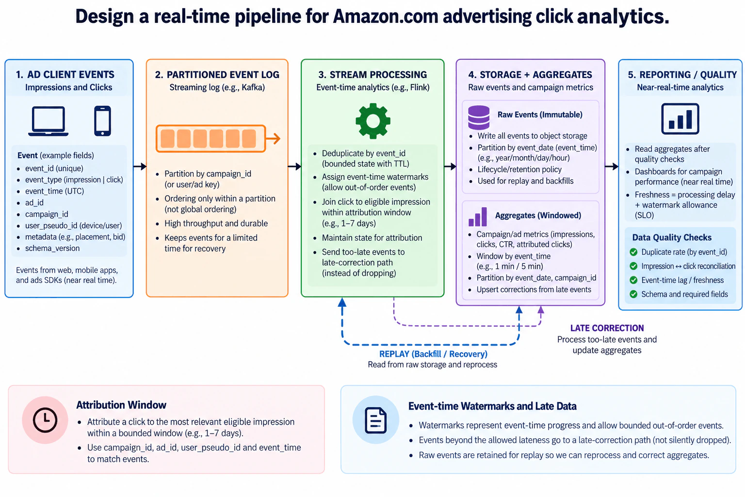
8. Design a real-time pipeline for Amazon.com advertising click analytics.Data PipelinesHardAmazon

Question Details

Design collection and processing of ad impressions and clicks for near-real-time reporting. Specify event identifiers, campaign metadata, partitioning, attribution windows, duplicate filtering, event-time watermarks, late corrections, raw retention, aggregates, replay, quality checks, and freshness guarantees.

Short Interview Answer (30-60 seconds)

I would capture each impression and click with a unique event_id and event_time, send the events through a partitioned streaming log, and process them by event time. The processor deduplicates events, attributes clicks to eligible impressions within a bounded window, and writes immutable raw data plus windowed aggregates. Watermarks balance freshness against late-data completeness, while late corrections, replay, and quality checks keep reporting accurate.

Detailed Explanation

The goal is to show advertising activity quickly without counting the same action twice or losing actions that arrive late. Every time an ad is shown or clicked, we record what happened, when it happened, which ad and campaign were involved, and a unique value for that action. We group related activity so it can be handled efficiently. Recent results become visible quickly, while the original records are kept so the numbers can be rebuilt or corrected later when delayed information arrives.

Useful Questions to Ask the Interviewer
  1. What reporting delay is acceptable for advertisers: seconds, one minute, or several minutes?
  2. What click-attribution window should we support, and can different campaigns use different windows?
  3. How long must raw events remain available for replay and historical correction?
  4. How late can an event arrive before it should stop updating the normal result and enter the late-correction path?
Design a real-time pipeline for Amazon.com advertising click analytics. diagram
How to Explain It in an Interview
1. Define the event contract

I would start by making every impression and click independently identifiable. Each event carries a unique event_id, event_type, UTC event_time, ad_id, campaign_id, user_pseudo_id, metadata such as placement or bid, and schema_version. The grain is one observed impression or one observed click per event record. event_id is the deduplication key, while event_time drives attribution and time windows. schema_version lets processing recognize which event contract it is reading instead of silently treating incompatible layouts as identical.

2. Ingest into a partitioned event log

Events from web, mobile apps, and ad SDKs move into the partitioned streaming log shown in the diagram. The log can be partitioned by campaign_id, or by a user/ad key when that key better keeps related records together for processing. Ordering exists only within an individual partition, not across the entire stream. The log provides durable high-throughput ingestion and keeps events for a limited recovery period. More partitions increase parallel processing capacity, but they also increase coordination overhead and can still perform poorly if the chosen key creates skew.

3. Process by event time and maintain attribution state

The stream-processing stage first deduplicates records by event_id using bounded state with a TTL. It then assigns event-time watermarks so bounded out-of-order events can still affect the appropriate results. For attribution, the processor joins a click to the most relevant eligible impression within the configured bounded attribution window, such as the one-to-seven-day example shown in the diagram. Matching uses campaign_id, ad_id, user_pseudo_id, and event_time. The processor keeps the bounded state required for deduplication and attribution rather than retaining unlimited stream history in memory.

4. Handle late data without silent loss

A watermark represents the processor's progress through event time and defines how much out-of-order arrival the normal path is prepared to accommodate. Events that arrive within the allowed lateness can still contribute to the expected event-time results. Events that are too late follow the separate late-correction path shown in the diagram instead of being silently discarded. That path processes the delayed information and upserts the affected aggregates. A wider lateness allowance can improve completeness, but it increases state requirements and makes recent results take longer to settle.

5. Store raw events and windowed aggregates

The storage stage keeps immutable raw events in object storage, partitioned by event_date derived from event_time, for example year, month, day, and hour. A lifecycle or retention policy controls how long they remain available, and those raw events are the source for replay and backfills. Separately, the processor produces windowed campaign/ad metrics such as impressions, clicks, CTR, and attributed clicks. These aggregates use event-time windows, such as the one-minute or five-minute examples in the diagram, and are partitioned by event_date and campaign_id. Late corrections upsert affected aggregate results.

6. Validate, report, and recover

Near-real-time reporting reads the aggregate results after the quality checks shown in the diagram. Those checks include duplicate rate by event_id, impression-to-click reconciliation, event-time lag and freshness, and schema and required-field validation. The freshness target includes both processing delay and the watermark allowance, so faster visibility and tolerance for late data must be balanced explicitly. If results must be rebuilt, the replay/backfill path reads retained immutable raw events and sends them back through the same stream-processing logic. That preserves the same deduplication, attribution, event-time, late-data, and quality rules during recovery.

Technical Approach
  1. Define one event record per impression or click with event_id, event_type, UTC event_time, ad_id, campaign_id, user_pseudo_id, metadata, and schema_version.
  2. Send events from web, mobile apps, and ad SDKs to a durable partitioned streaming log.
  3. Partition by campaign_id or a suitable user/ad key and assume ordering only within each partition.
  4. Deduplicate by event_id using bounded state with TTL.
  5. Apply event-time watermarks and maintain bounded attribution state.
  6. Match clicks to the most relevant eligible impressions within the configured attribution window using campaign_id, ad_id, user_pseudo_id, and event_time.
  7. Send too-late events through the late-correction path.
  8. Persist immutable raw events partitioned by event_date for replay and backfills.
  9. Produce event-time windowed campaign/ad aggregates and upsert corrections from late events.
  10. Run duplicate, reconciliation, freshness, schema, and required-field checks before near-real-time reporting.
Practical Insights

The benefit is that streaming gives advertisers fresh results while event-time processing handles delayed events correctly. The downside is more state and operational complexity. More event-log partitions can increase parallelism, but too many partitions add coordination cost, and an uneven key can create hot partitions. Longer deduplication and attribution windows catch more delayed or repeated events, but they require more processing state. A larger watermark allowance improves late-data completeness, but recent reports take longer to settle. Immutable raw retention makes replay and backfills possible, but it increases storage and replay-compute cost. Precomputed aggregates make reporting fast, but late corrections require controlled upserts. We accept these costs because correctness, recovery, and predictable freshness are important requirements.

Why Interviewers Ask This

This question tests whether a candidate can reason about correctness in a real streaming analytics system instead of only naming tools. The interviewer wants to see good judgment about event identity, partitioning and ordering, event time, duplicates, attribution, late arrivals, replay, quality, and freshness. It also tests whether the candidate understands the trade-off between fast reporting and waiting longer for more complete data, and whether historical recovery can reproduce trustworthy business results.

Common interview mistakes

Common mistakes are using processing time instead of event time for attribution, assuming global ordering across the event log, or deduplicating without a bounded retention rule. Another mistake is treating broker delivery behavior as proof of exactly-once business results. Candidates may also drop events that arrive after the normal lateness bound instead of using the shown late-correction path. Omitting immutable raw retention makes replay and backfills difficult. Finally, reporting aggregates merely because processing completed is unsafe; the design requires duplicate, reconciliation, freshness, schema, and required-field checks before consumers rely on the results.

Interview tip

Explain the design in the same left-to-right order as the diagram: event contract, partitioned log, event-time processing, raw and aggregate storage, then reporting and quality. Spend the most time on correctness: event_id deduplication, partition-scoped ordering, attribution state, watermarks, late corrections, and replay. State the central trade-off clearly: allowing more lateness improves completeness but makes recent results take longer to become stable.

Interviewer may ask next
What would you change if advertisers required much fresher reporting while event arrival patterns stayed the same?

I would keep the same architecture and tighten the freshness contract rather than replace the pipeline. The affected parts are the event-time watermark, aggregate window size, and reporting visibility point. I would use smaller event-time windows where practical and reduce the normal watermark allowance only as far as the accepted late-arrival behavior permits. Events inside the new bound would continue through normal event-time processing, while events beyond it would still use the existing late-correction path. The raw immutable event store, event_id deduplication, attribution keys, attribution window, and replay path would remain unchanged.

Validation would pay particular attention to end-to-end freshness because the smaller delay budget leaves less room for processing lag. The same duplicate, reconciliation, schema, required-field, and event-time freshness checks would remain before reporting. Recovery would still replay raw events through the same processing logic. The main downside is that a tighter watermark can classify more valid events as late, causing more aggregate corrections and making the newest numbers less stable. I would accept that only if the business explicitly prefers faster provisional results.

How would you handle a processing bug that produced incorrect campaign aggregates for several hours?

I would rebuild the affected period from immutable raw events rather than manually changing dashboard values. The live collection and partitioned-log path can remain unchanged. I would select the affected raw event_date partitions and use the replay/backfill path shown in the diagram to send those records back through the stream-processing logic. The replay must use the same event_id deduplication, event-time behavior, attribution keys, attribution window, and late-correction rules as normal processing. Corrected output would upsert the affected campaign/date aggregates.

Before the rebuilt results are used for reporting, I would run the same duplicate-rate, impression-to-click reconciliation, event-time freshness, schema, and required-field checks. I would also reconcile the replayed input range with the corrected output so the recovery is verifiable. The main downside is additional processing and storage-read load during replay. I would therefore keep the historical rebuild controlled so it does not overwhelm the normal near-real-time path. No separate calculation architecture is needed.

9. Explain when to use Amazon S3, Amazon Redshift, Amazon RDS, and Amazon DynamoDB for data storage.Cloud Data PlatformsEasyAmazon

Question Details

Compare these services by data shape, access pattern, latency, transaction support, analytical scans, scale, durability, and cost. Identify the role each can play and why object storage, a columnar warehouse, a relational database, and a key-value database are not interchangeable.

Short Interview Answer (30-60 seconds)

I would choose storage from the workload: S3 for objects and data-lake files, Redshift for analytical SQL scans, RDS for relational OLTP, and DynamoDB for high-scale low-latency key access. The main trade-off is matching the data model and access pattern instead of forcing one service to handle every workload.

Detailed Explanation

Applications, business systems, databases, logs, files, and data teams produce data that has very different storage needs. Some workloads need cheap durable objects, some need large analytical scans, some need relational transactions, and others need predictable key-based access at high scale. One storage system cannot serve all of those patterns equally well. The design therefore puts a workload-selection decision in front of four specialized AWS services. The choice is driven by data shape, access pattern, latency, transaction support, analytical scans, scale, durability, and cost. The goal is to select the right storage behavior without pretending the four services are interchangeable.

Useful Questions to Ask the Interviewer
  1. Is the dominant workload object storage, analytical SQL, relational OLTP, or key-value and document access?
  2. What latency does the consumer need: operational millisecond access, single-digit-millisecond key access, or analytical query latency?
  3. Does the workload need relational joins and multi-row transactions, DynamoDB transactions, or mainly independent object operations?
  4. Will users run large scans and aggregations, or mostly retrieve known records and objects?
  5. Which cost boundary matters most: stored objects and requests, warehouse compute and storage, relational database compute and storage, or request and capacity consumption?
Explain when to use Amazon S3, Amazon Redshift, Amazon RDS, and Amazon DynamoDB for data storage. diagram
How to Explain It in an Interview
1. Start with the storage-selection decision

The producer side contains web and mobile applications, business systems and databases, logs, events and files, plus data engineering and analytics teams. Their data reaches a central decision point labeled to choose storage based on workload and access pattern. From there, S3, Redshift, RDS, and DynamoDB are alternative storage choices. They are not four mandatory stages in one pipeline.

This separation is important because each service owns a different primary responsibility. A poor choice normally appears as the wrong data model, expensive access, poor latency, awkward transaction logic, or inefficient analytical scans. The trade-off is that a platform may use several storage services, but each workload gets a storage system designed for its dominant access pattern.

2. Use Amazon S3 for files and objects

Amazon S3 is the object-storage branch. It fits files and objects of many types, including raw and curated data-lake files, backups, exports, and archival data. Applications retrieve or write objects by key, and analytical engines can read collections of S3 objects when the data must be queried.

S3 Standard is designed for 99.999999999% durability, and S3 can store very large amounts of data without the producer managing database servers. Frequently accessed S3 storage classes provide millisecond object access, but S3 is not a relational OLTP database and does not provide the relational transaction model expected from RDS. It is also not itself a columnar data warehouse. Large analytical queries over S3 require a separate analytics engine.

The green path in the diagram leads from the storage decision to S3 and then toward BI and analytics consumers. The intended role is durable object and lake storage that analytical tools can consume. Its cost model is mainly based on storage class, stored data, requests, retrieval behavior, and related usage rather than continuously running relational database compute.

3. Use Amazon Redshift for analytical SQL and large scans

Amazon Redshift is the columnar data-warehouse branch. It is designed for structured analytical tables, SQL queries, aggregations, and large scans. This is the right choice when users need business intelligence, reporting, data warehousing, or other analytical workloads that read substantial portions of large datasets.

Redshift supports database transactions and provides SNAPSHOT and SERIALIZABLE isolation options, but its main role is analytics rather than high-frequency OLTP. Its columnar architecture and analytical execution model make large scans a much better fit than they are in an operational relational database.

The diagram describes Redshift as petabyte-scale, with managed backups and a Multi-AZ deployment option. Multi-AZ is an availability option rather than something every Redshift deployment automatically uses. Its cost boundary is warehouse compute plus storage and related usage. The purple path terminates at application users in the diagram, representing users or applications consuming analytical results from the warehouse.

4. Use Amazon RDS for relational OLTP

Amazon RDS is the managed relational-database branch. It fits normalized relational rows and applications that need SQL, joins, constraints, and full ACID transaction behavior. It is the strongest choice among these four when an operational system needs relational integrity and transactional updates.

RDS is intended for OLTP-style access with database latency appropriate for operational applications. It can support reporting, but the diagram correctly marks large-scale analytical scans as limited because a transactional database should not be treated as a columnar warehouse. If reporting becomes dominated by broad scans and aggregations, Redshift is the better analytical boundary.

RDS can use Multi-AZ deployments for high availability and supports automated backups and point-in-time recovery within the configured backup-retention behavior. Scaling depends on the selected database engine and deployment model. Its cost is mainly database compute, storage, backups, I/O, and related managed-database usage. The blue path in the diagram leads to reports and dashboards, which is reasonable for operational reporting that remains within RDS's workload limits.

5. Use Amazon DynamoDB for high-scale key-value access

Amazon DynamoDB is the key-value and document database branch. It fits applications with known key-based access patterns that need consistent single-digit-millisecond performance at very large scale. The diagram gives examples such as sessions, carts, profiles, and other high-scale operational workloads.

DynamoDB supports key-value and document models and native ACID transactions. It does not support relational joins, so a relational schema that depends heavily on joins is a better fit for RDS. DynamoDB is also not designed as a scan-heavy analytical warehouse, so broad analytical scans should normally move to an analytical system rather than become the primary DynamoDB access pattern.

By default, DynamoDB replicates table data across three Availability Zones within an AWS Region for resilience. Its cost model can use on-demand request pricing or provisioned capacity. The orange path leads to operational applications because DynamoDB is strongest when applications issue predictable key-based reads and writes rather than warehouse-style queries.

6. Compare the services by the required dimensions

For data shape, S3 stores objects and files, Redshift stores columnar analytical tables, RDS stores relational tables, and DynamoDB stores key-value or document items.

For access pattern, S3 uses object-oriented reads and writes, Redshift serves analytical SQL and large aggregations, RDS serves transactional SQL and joins, and DynamoDB serves primary-key and index-based reads and writes.

For latency, RDS and DynamoDB target operational access patterns. DynamoDB is specifically designed for consistent single-digit-millisecond performance. Redshift accepts analytical query latency because it optimizes for large data processing rather than point lookups. S3 provides object access rather than database-query latency.

For transactions, RDS provides the traditional relational ACID model. DynamoDB supports ACID transactional operations across items and tables within the supported transaction boundary. Redshift supports transactions for warehouse workloads. S3 object operations do not turn S3 into an OLTP transaction database.

For analytical scans, Redshift is the primary fit. S3 can hold the data being analyzed, but an analytics engine performs the query. RDS is a poor primary choice for warehouse-sized scans, and DynamoDB should not be designed around full-table analytical scanning.

For scale and durability, each service scales differently. S3 scales object storage and provides very high durability. Redshift scales analytical warehouse capacity. RDS scales within relational database and deployment boundaries. DynamoDB automatically scales key-oriented workloads according to its configured capacity mode and partitioned architecture while replicating data across Availability Zones.

For cost, S3 is object-storage and request oriented, Redshift is warehouse-compute and storage oriented, RDS is managed relational-compute and storage oriented, and DynamoDB is request or provisioned-capacity oriented. There is no universally cheapest option because the billing unit and workload are different.

7. Handle failures according to the storage service

The four services also have different failure and recovery behavior. With S3, a failed analytical job can normally retry against the stored objects; a query failure is separate from object durability. With Redshift, failed queries may need to be retried, and backups or a Multi-AZ deployment can address different recovery and availability needs. With RDS, automated backups provide restore and point-in-time recovery, while Multi-AZ can provide database failover. With DynamoDB, the service automatically replicates data across three Availability Zones, while backup and restore are separate capabilities.

The application or data team still owns validating that recovered or retried work produced correct business results. None of the four branches in this diagram establishes multi-Region disaster recovery, so I would not claim that requirement is solved unless it is explicitly designed.

8. Keep the cost models separate

The bottom cost callout summarizes an important interview point. S3 charges around object storage, storage classes, requests, retrieval, and related usage. Redshift cost is tied to warehouse compute and storage. RDS cost is tied to managed database compute, storage, I/O, backups, and related features. DynamoDB cost is tied primarily to request or provisioned capacity, storage, and optional features.

That means the correct cost comparison starts from the workload. Storing a large archive in an always-running relational database pays for capabilities the archive does not need. Using object storage for a transactional relational application avoids database compute but also removes the relational database behavior the application requires.

9. Treat the four services as complementary

The final design principle is that S3, Redshift, RDS, and DynamoDB are complementary rather than interchangeable. S3 solves object storage. Redshift solves columnar analytical warehousing. RDS solves relational transactions. DynamoDB solves high-scale key-value and document access.

A broader AWS data platform may use several of them at the same time for different data products. That still does not mean every record must flow through all four services. The central workload decision remains the key architectural boundary: choose the storage service whose data model, access pattern, latency, transaction behavior, analytical capability, scale, durability, and cost structure fit the workload.

Technical Approach
  1. Identify the producer and consumer requirement.
  2. Classify the data shape as files or objects, analytical tables, relational rows, or key-value and document items.
  3. Identify the dominant access pattern: object retrieval, analytical scans, transactional SQL, or key lookup.
  4. Check latency requirements.
  5. Check whether relational or multi-item transactions are required.
  6. Determine whether broad analytical scans and aggregations are central to the workload.
  7. Compare the required scaling and durability behavior.
  8. Compare the cost boundary: S3 storage classes and requests, Redshift warehouse compute and storage, RDS database compute and storage, or DynamoDB requests and capacity.
  9. Select the primary service that matches the workload instead of chaining all four alternatives together.
  10. Reevaluate the boundary if the access pattern changes.
Practical Insights

There is no useful Big-O calculation for this storage-selection question. The important complexity is scale, latency, operations, and cost. S3 can hold very large object datasets without managing database servers, but analytical queries need a separate engine. Redshift adds warehouse compute that is useful for large scans but has its own compute cost and concurrency limits. RDS provides relational transactions and joins, but its capacity and scaling remain database-engine concerns. DynamoDB removes most server management and can scale key-based traffic, but the partition key and access pattern must be designed correctly. Storage growth, request volume, query concurrency, backup behavior, network transfer, and provisioned or idle compute can all change the cost. The likely bottleneck depends on the branch: analytical query capacity in Redshift, relational database resources in RDS, access-pattern and partition design in DynamoDB, or the external query engine when analyzing S3 data.

Why Interviewers Ask This

Interviewers want to know whether a Data Engineer can map a workload to the correct storage abstraction instead of treating every AWS storage service as interchangeable. The important judgment is recognizing when the problem needs object storage, a columnar warehouse, a relational transactional database, or a key-value and document database, and explaining the consequences for latency, transactions, analytical scans, scale, durability, and cost.

Common interview mistakes

A common mistake is describing all four services as databases that mainly differ by scale. S3 is object storage, Redshift is an analytical warehouse, RDS is a managed relational database, and DynamoDB is a key-value and document database. Another mistake is using S3 as though it provided relational OLTP transactions, using RDS as the primary store for warehouse-sized scans, or choosing DynamoDB simply because it scales without designing its keys and access patterns. It is also wrong to assume Redshift should replace RDS merely because Redshift supports transactions. Finally, do not describe the four branches as a mandatory S3-to-Redshift-to-RDS-to-DynamoDB pipeline. The diagram uses them as alternative choices selected by workload and access pattern.

Interview tip

Lead with the access pattern instead of listing AWS products. Explain what the workload needs, map that requirement to S3, Redshift, RDS, or DynamoDB, and compare data shape, latency, transactions, analytical scans, scale, durability, and cost. Finish by stating that the services are complementary rather than interchangeable.

Interviewer may ask next
What would you do if an RDS workload starts producing reporting queries that scan large portions of its relational tables?

I would keep RDS as the transactional source because the application still needs relational OLTP behavior. I would separate the scan-heavy reporting workload and serve it from the analytical side, normally Redshift when the requirement is large SQL scans and aggregations. That prevents analytical queries from competing with operational transactions for the same relational database resources. If files or historical exports are also needed, S3 can hold them as durable objects, but S3 itself is not the warehouse query engine. I would validate that the analytical data is sufficiently fresh and reconcile it with the transactional source before consumers rely on it.

What changes if the application needs very high request scale with predictable key lookups but also needs complex joins and large analytical scans?

I would not force all three access patterns into DynamoDB. DynamoDB remains the operational store for the high-scale key-based requests because that matches its design. If the application has transactional relationships that genuinely require relational joins and constraints, that data belongs in an RDS relational model. Large analytical scans and aggregations belong in Redshift. S3 can hold raw, historical, exported, or lake data when object storage is useful. These become separate workload boundaries rather than one sequential storage chain, and each service is selected for the behavior it provides best.

10. How would you choose between Amazon Redshift and S3 with Athena for an analytics workload?Cloud Data PlatformsMediumAmazon

Question Details

Evaluate concurrency, scan volume, freshness, transformation needs, table format, performance predictability, administration, and cost. Explain when a warehouse is appropriate and when querying partitioned object files directly is the simpler platform choice.

Short Interview Answer (30-60 seconds)

I would keep curated data in S3 and choose the query engine by workload shape. Redshift fits sustained, high-concurrency BI and complex transformations with predictable performance, while Athena fits ad hoc analysis of fresh, partitioned S3 data when simpler operations and scan-based cost matter more.

Detailed Explanation

The platform serves producers and analytics consumers that have different query patterns but share the same curated S3 data foundation. Building a separate analytics stack for every source or consumer would duplicate storage, governance, metadata, monitoring, and operational work. The main decision is therefore the serving engine. Sustained concurrency, repeated large scans, complex SQL, and predictable performance favor Redshift. Intermittent exploration, direct access to fresh S3 data, good partition pruning, and lower administration favor Athena. The design keeps storage and shared operational controls reusable while letting each workload use the query engine that best matches its behavior.

Useful Questions to Ask the Interviewer
  1. Is the workload mainly scheduled dashboards and repeated BI queries, or intermittent exploratory SQL?
  2. How much query concurrency do we expect, and do many users need predictable performance at the same time?
  3. Are queries repeatedly scanning large portions of the data, or can they prune well-partitioned S3 data effectively?
  4. How fresh must results be after curated data becomes available in S3?
  5. Do we need complex joins and transformations as a normal part of analytics, or mostly direct reads of curated data?
  6. Are the S3 datasets stored in efficient columnar formats such as Parquet or ORC, or represented as Iceberg tables?
  7. Is the team willing to operate warehouse capacity, or is simpler administration more important?
  8. Is cost driven more by sustained analytics capacity or by intermittent query activity and data scanned?
How would you choose between Amazon Redshift and S3 with Athena for an analytics workload? diagram
How to Explain It in an Interview
  1. Start with the workload decision

I would treat Redshift and Athena as alternative serving paths, not as sequential processing stages. The central workload decision looks at concurrency, scan volume, transformations, performance predictability, freshness, administration, and cost. High concurrency, repeated or large scans, complex transformations, and a stronger need for predictable performance point toward Redshift. Ad hoc or intermittent SQL over fresh, partitioned S3 data with simpler operations points toward Athena.

The workload can change over time, so I would observe query latency, concurrency, scan behavior, and cost and reconsider the placement when those characteristics change.

  1. Keep Amazon S3 as the shared data foundation

The producer side includes operational databases, application logs, streaming events, SaaS data, and other sources. Data is ingested into a shared Amazon S3 data lake and represented as curated, partitioned analytics data.

The diagram shows Parquet or ORC as columnar file choices and Iceberg as an optional table format. Partitioning and compression are especially important for Athena because they can reduce unnecessary scanning. The same S3 foundation can support the Athena query-in-place path and data used by Redshift-oriented analytics.

The shared storage layer means the platform does not need a completely separate data foundation for every query engine. Storage problems, stale curated data, or poor physical layout can affect downstream analytics independently of which serving engine is chosen.

  1. Choose Amazon Redshift for warehouse-style workloads

I would choose Redshift when many BI users query concurrently, queries repeatedly scan large datasets, complex SQL and transformations are common, or consumers need more predictable performance.

Redshift provides workload management, and concurrency scaling can add capacity for increases in concurrent query demand. That makes it a strong fit for steady BI workloads and dashboards.

For provisioned Redshift, the team accepts more warehouse administration. Redshift Serverless reduces cluster-management work, so I would not describe Redshift as always requiring manual cluster operation. The cost model also differs from Athena because Redshift can use provisioned or Serverless compute together with managed storage.

If the Redshift workload becomes small and intermittent, I would reconsider whether the warehouse path is still justified.

  1. Choose Amazon Athena for query-in-place analytics

Athena queries data directly in S3, so this path does not require loading the data into a separate warehouse before querying it. I would prefer it for ad hoc or intermittent analysis when curated data is already well partitioned and users want to query recently available S3 data directly.

Athena works especially well when queries can prune partitions and read efficient formats such as Parquet or ORC. It can also query Iceberg tables, matching the optional Iceberg representation shown in the diagram.

Operationally, Athena is simpler because there is no analytics warehouse cluster to manage for this path. With per-query billing, cost is tied to data scanned. Athena also supports reserved compute capacity. Concurrency quotas still matter, and when reserved capacity is busy, additional queries assigned to that capacity can queue until capacity becomes available.

If an Athena workload starts producing high sustained concurrency, broad repeated scans, or a stronger need for predictable performance, that is a signal to reconsider Redshift.

  1. Match each consumer to the correct serving pattern

The diagram shows business users, applications, analysts, data scientists, BI dashboards, and ad hoc reporting as consumers. Both Redshift and Athena expose SQL, but they serve different workload shapes.

Redshift is the stronger choice for steady BI and dashboard traffic. Athena is the simpler choice for exploratory and intermittent SQL over S3. I would not place a sustained high-concurrency dashboard workload on Athena merely because the source data is stored in S3, and I would not require a warehouse for occasional exploratory queries merely because Redshift is available.

  1. Keep governance, metadata, and operations shared

The bottom platform layer provides shared identity and access control, data catalog and metadata, monitoring and cost controls, and platform operations. These capabilities support the analytics platform without becoming the normal business-record data path.

Identity and access controls determine who can access the analytics data. The diagram also includes row and column controls. The catalog stores definitions, schema, and lineage metadata rather than the production records themselves. Monitoring and cost controls collect usage, query metrics, and budget signals. Platform operations covers the shared security, support, and operational responsibilities shown in the design.

The dashed connections represent metadata, policy, and monitoring relationships. I would not describe those dashed paths as carrying production records.

  1. Separate freshness from performance predictability

Athena can query curated data directly from S3, so it avoids a separate warehouse-load dependency for that serving path. That is useful when access to recently available S3 data is important.

However, direct access does not mean every Athena query has identical latency. Query behavior still depends on factors such as partition pruning, amount of data scanned, query shape, and available capacity.

Redshift is more appropriate when the workload benefits from a warehouse environment designed around repeated analytics, workload management, concurrency, and more predictable performance. The trade-off is greater warehouse-oriented capacity and operational responsibility compared with the simpler Athena path.

  1. Compare cost using the real access pattern

For Athena, I would look at how much data queries scan and whether the workload uses per-query billing or reserved capacity. Partitioning, compression, and selective columnar reads can reduce unnecessary scanning. This makes Athena attractive for intermittent workloads where maintaining warehouse-oriented capacity is unnecessary.

For Redshift, I would consider its provisioned or Serverless compute model and managed storage together with the operational value it provides for sustained analytics.

I would not say Athena is always cheaper or Redshift is always more expensive. A frequently repeated Athena query that scans large amounts of data can be a poor fit, while a well-utilized warehouse can be reasonable for sustained high-concurrency analytics.

  1. Handle failures at the correct boundary

If curated S3 data is late or incorrect, both serving paths can expose stale or incorrect results because they depend on that shared data foundation. That is a data-layer problem rather than an Athena-specific or Redshift-specific failure.

If Athena capacity is busy, affected Athena queries can wait or encounter concurrency-related limits while the Redshift path remains a separate workload boundary. Operators should inspect query state, concurrency, scan volume, and capacity signals before changing the platform choice.

If Redshift experiences queue pressure or poor query performance, operators should inspect workload management, concurrency, query behavior, and available warehouse capacity. That does not imply that the S3 data itself has failed.

  1. Keep the design reusable

The reusable platform foundation is the shared S3 storage, governance, metadata, monitoring, cost controls, and operational model. Producer teams can feed different types of data into the platform, while analysts, data scientists, applications, and BI users can consume it through the engine that matches their workload.

The diagram does not define a separate self-service provisioning portal, formal tenant isolation model, region strategy, or migration control plane, so I would not invent those details. The important reusable decision is to keep the common data and governance foundation shared while allowing Redshift and Athena to remain independent serving choices.

Technical Approach
  1. Identify whether the workload is sustained BI, repeated analytical SQL, or intermittent exploration.
  2. Evaluate expected concurrency and whether simultaneous users need predictable performance.
  3. Examine scan behavior: repeated large scans strengthen the Redshift case, while selective scans over well-partitioned S3 data strengthen the Athena case.
  4. Evaluate freshness: direct S3 querying is useful when curated data should be queryable without a separate warehouse-load step.
  5. Evaluate transformation complexity: frequent complex joins and transformations favor Redshift.
  6. Check the S3 physical and table representation, especially partitioning, compression, Parquet or ORC, and optional Iceberg.
  7. Compare administration: provisioned Redshift has more warehouse-management responsibility, Redshift Serverless reduces cluster management, and Athena has no warehouse cluster to operate for the query path.
  8. Compare cost using actual behavior: Athena data scanned or reserved capacity versus Redshift provisioned or Serverless compute and managed storage.
  9. Choose one normal serving path for the workload rather than chaining Redshift and Athena together.
  10. Monitor concurrency, latency, scan volume, freshness, and cost and revisit the decision when the workload changes.
Practical Insights

The biggest scaling concern in this design is query behavior. Redshift is better suited to sustained concurrency and repeated heavy analytical queries because it has warehouse workload-management and concurrency features. Athena avoids operating a warehouse cluster, but broad scans increase work and scan-based cost, and concurrency or busy reserved capacity can affect query execution. S3 storage can grow independently of either query engine. Good partitioning, compression, and columnar formats reduce Athena scan volume. Athena can query curated S3 data without a separate warehouse-load step. Redshift adds more warehouse-oriented operating responsibility, although Serverless reduces cluster management. Moving a workload between the two mainly changes serving, transformations, query behavior, validation, and consumer cutover while the shared S3 foundation can remain in place.

Why Interviewers Ask This

Interviewers want to see whether I can choose an analytics platform from workload behavior instead of choosing a service by habit. The key judgment is how concurrency, scan volume, freshness, transformation complexity, file or table format, performance predictability, administration, and cost change the decision between a warehouse and querying data directly in object storage.

Common interview mistakes

A common mistake is saying Redshift is always faster or Athena is always cheaper without explaining the workload. Another is drawing or describing Athena and Redshift as sequential stages even though they are alternative serving paths in this design. Candidates also forget concurrency, scan volume, freshness, transformations, partitioning, file format, performance predictability, administration, and cost. It is also incorrect to describe the catalog as storing production records or the dashed governance paths as business-data flows. Another mistake is ignoring Athena reserved capacity or claiming that Redshift always requires cluster management even though Redshift Serverless reduces that responsibility.

Interview tip

Lead with workload shape rather than product names. State that S3 is the shared data foundation, then compare Redshift and Athena using concurrency, scan pattern, freshness, transformation complexity, predictability, administration, and cost. Make it explicit that they are alternative serving paths and explain what workload changes would make you switch.

Interviewer may ask next
What would you do if an Athena workload gradually became a high-concurrency dashboard workload with repeated large scans?

I would first confirm the change using query concurrency, scan volume, latency, queue behavior, and cost. If the workload is now sustained and repeatedly scans large datasets, I would move that consumer path toward Redshift rather than keep treating it as ad hoc exploration. The curated S3 foundation can remain shared. I would reproduce the required serving logic in Redshift, compare query results during the transition, and cut consumers over only after the results are consistent. The reason for the move is that concurrency, repeated scans, and predictable performance now matter more than the operational simplicity of querying S3 directly.

What if freshness becomes the most important requirement and analysts need to query curated data as soon as it is available in S3?

Assuming the curated S3 data is ready for consumption, I would favor Athena for workloads that can query it directly. That avoids a separate warehouse-load dependency before those queries can run. I would keep the data well partitioned and use an efficient format such as Parquet or ORC, or Iceberg when that table format is appropriate. I would still monitor scan volume, latency, concurrency, and cost. If those fresh-data queries later become highly concurrent, repeatedly scan large datasets, or require more predictable performance, I would reconsider a Redshift serving path.

More questions load as you scroll

Disclaimer: This interview guide is for educational and informational purposes only. It is designed to help readers prepare, but it does not guarantee any interview result, hiring decision, offer, or outcome. Interview questions, hiring criteria, and preferred answers can vary by employer, interviewer, industry, location, and time. The examples and explanations reflect the authors' research and judgment, are provided without warranties of any kind, and should not be treated as the only correct approach. Diagrams are simplified illustrations intended to highlight the main components and their interactions; actual systems and implementations may be more complex. Alternative approaches may be equally valid or better suited to a particular question, context, or interviewer. To the fullest extent permitted by applicable law, the author, contributors, and publisher are not liable for decisions made, actions taken, or losses incurred based on this guide.

Company Notice: This guide is an independent educational resource and is not affiliated with, endorsed by, sponsored by, or approved by the company named in this guide. Company names are used only to identify interview experiences commonly reported by candidates. Interview practices can change without notice, and inclusion of company-specific content does not mean these questions are official, complete, or guaranteed to be asked. To the fullest extent permitted by law, the author, contributors, and publisher are not responsible for outcomes related to use of this material.

Content Accuracy and Verification: To the fullest extent permitted by applicable law, we do not represent or warrant that interview guides, questions, answers, examples, or diagrams are accurate, complete, current, error-free, or suitable for any particular purpose. You are responsible for independently reviewing and verifying the information before relying on it.