15 Netflix Data Engineer Interview Questions & Answers

netflix icon

Questions with Detailed ExplanationsWith Detailed Explanations

(Last Updated: September 8, 2026)

1. Define a canonical fact table for Netflix member playback telemetry.Data ModelingEasyNetflix

Question Details

Specify the row grain, stable event identity, keys, and minimum columns needed to calculate total watch time by title and day across devices while remaining correct under client retries. Distinguish member, profile, device, session, content, event time, ingestion time, duration, schema version, and correction metadata, and state how a deterministic current view relates to immutable source history.

Short Interview Answer (30-60 seconds)

I would keep one current fact row per logical event_id. Client retries reuse that ID, while immutable history stores every delivery. Corrections are selected deterministically, and watch time sums duration_ms for ACTIVE rows by content_id and the UTC date of event_time_utc.

Detailed Explanation

See the Code while reading this explanation.

The goal is to count viewing time correctly even when the same viewing record arrives more than once. Each real playback event needs one stable identity, while every received copy should still be kept for traceability. Later corrections must change the current meaning without deleting the original history. The reporting view should contain only one selected version of each playback event. Daily totals must use when playback actually happened, not when the data arrived, so retries and late deliveries do not move viewing time to another day or count the same playback twice.

Useful Questions to Ask the Interviewer
  1. Should every retry of the same logical playback event reuse the same event_id?
  2. Which event_status values exist, and should only ACTIVE events contribute to watch time?
  3. Is event_time_utc already normalized to UTC before it reaches this model?
  4. Are member_id, profile_id, device_id, session_id, and content_id stable upstream identifiers?
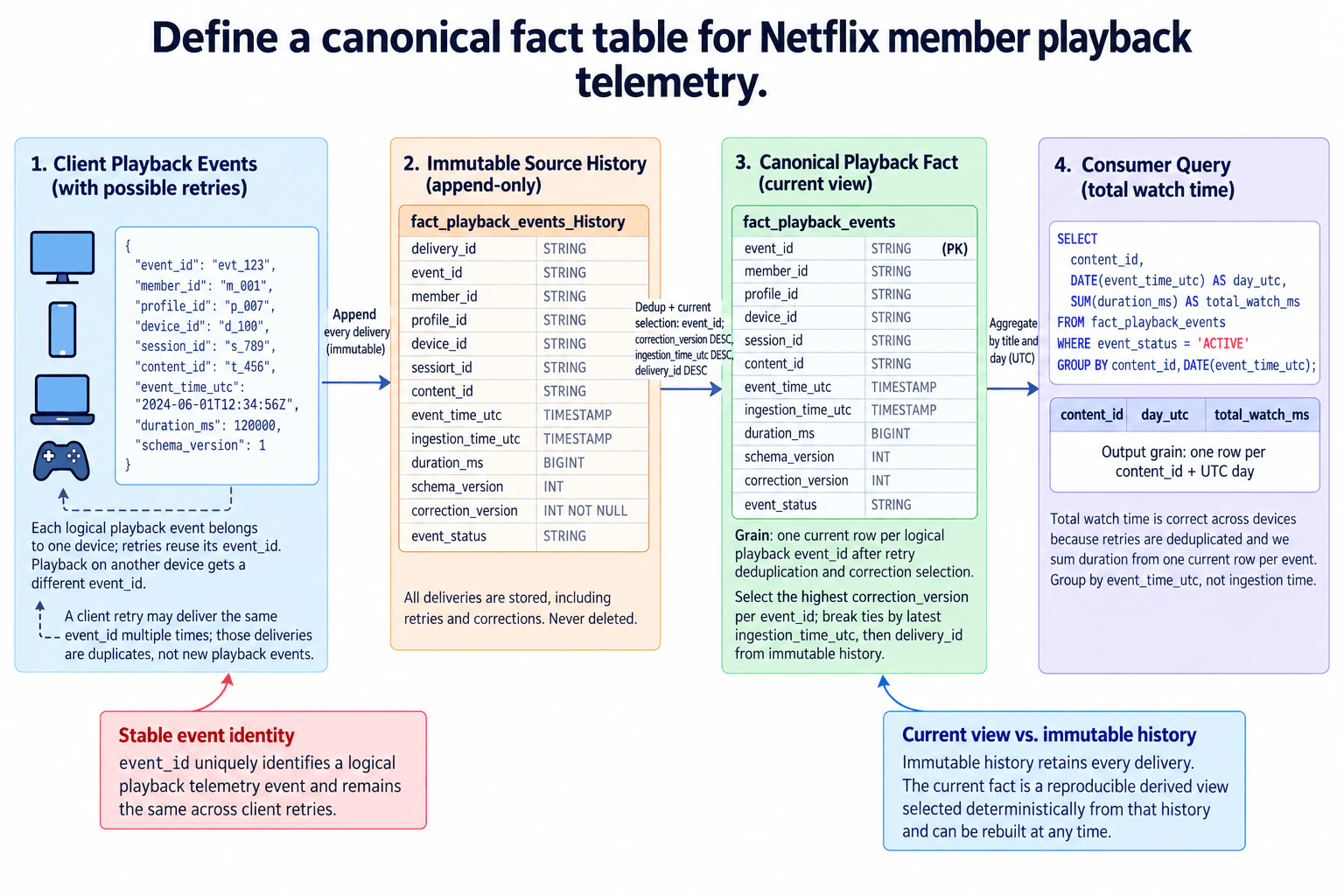
Define a canonical fact table for Netflix member playback telemetry. diagram
How to Explain It in an Interview

Start with the grain. The canonical fact, fact_playback_events, has one current row per logical playback event_id after retry deduplication and correction selection. event_id is the primary key of this current view. A retry of the same logical event reuses the same event_id. Playback on another device is a different logical playback event and therefore gets a different event_id.

Keep immutable source history separately in fact_playback_events_history. Its grain is one row per received delivery. delivery_id identifies a particular immutable delivery, while event_id identifies the logical playback event. Multiple history rows can therefore share one event_id when the client retries or when a corrected version is delivered. History is append-only and is not deleted.

The canonical current fact contains event_id, member_id, profile_id, device_id, session_id, content_id, event_time_utc, ingestion_time_utc, duration_ms, schema_version, correction_version, and event_status. member_id identifies the member, profile_id the viewing profile, device_id the playback device, session_id the playback session, and content_id the title or content. event_time_utc records when playback occurred. ingestion_time_utc records when that delivery reached the data platform. duration_ms is the watch-time measure. schema_version identifies the event schema version. correction_version orders corrections of the same logical event. event_status controls whether the selected event contributes to the metric.

Build the current view deterministically from immutable history. For each event_id, choose the row with the highest correction_version. If rows still tie, choose the latest ingestion_time_utc. If they still tie, use delivery_id descending as the final deterministic tie-break. The current fact is therefore a reproducible derived view that can be rebuilt from immutable history.

For total watch time, query the canonical current fact rather than immutable delivery history. Filter to event_status = 'ACTIVE', group by content_id and DATE(event_time_utc), and sum duration_ms. The result grain is one row per content_id and UTC day. Retries do not inflate the metric because only one current row exists per logical event_id.

No specific database engine was named. The SQL therefore follows the warehouse-style syntax shown in the approved diagram and assumes event_time_utc is stored as a UTC timestamp for DATE(event_time_utc) to represent the UTC playback day.

Technical Approach
  1. Declare the canonical current fact grain as one row per logical event_id.
  2. Require retries of the same logical playback event to reuse event_id.
  3. Append every received delivery to immutable history with its own delivery_id.
  4. Keep correction_version and event_status with each delivered version.
  5. For each event_id, select correction_version descending, then ingestion_time_utc descending, then delivery_id descending.
  6. Expose that selected row as the canonical current fact.
  7. For watch-time reporting, filter to event_status = 'ACTIVE', group by content_id and the UTC date of event_time_utc, and sum duration_ms.
Practical Insights

Immutable history uses more storage because it keeps every delivery, including retries and corrections. Rebuilding the current fact requires grouping or ordering history rows by event_id to select one row for each logical playback event. The current fact is smaller because it has one selected row per event_id. Daily reporting then filters ACTIVE rows and aggregates duration. The tradeoff is extra history storage and transformation work in exchange for retry safety, auditability, deterministic corrections, and reproducible watch-time metrics.

Code
-- Read the canonical current fact so retry deliveries are not double-counted.
SELECT
  content_id,
  -- event_time_utc represents when playback occurred and defines the UTC reporting day.
  DATE(event_time_utc) AS day_utc,
  -- duration_ms is additive across the selected logical playback events.
  SUM(duration_ms) AS total_watch_ms
FROM
  fact_playback_events
  -- Only ACTIVE current events contribute watch time.
WHERE
  event_status = 'ACTIVE'
  -- Result grain: one row per content_id and UTC playback day.
GROUP BY
  content_id,
  DATE(event_time_utc);
Why Interviewers Ask This

This tests whether the candidate can declare a precise fact-table grain, separate logical playback identity from physical deliveries, handle duplicate client retries safely, model corrections without losing immutable history, distinguish event time from ingestion time, and define a deterministic analytical view that produces correct watch-time totals across devices.

Common interview mistakes

Using ingestion_time_utc instead of event_time_utc for the reporting day can assign late-arriving playback to the wrong day. Aggregating immutable history directly can double-count client retries. Giving every retry a new event_id prevents correct deduplication. Overwriting history removes auditability and makes reconstruction harder. Selecting a correction without deterministic ordering can produce inconsistent rebuilds. Summing non-ACTIVE current rows can inflate watch time. Another mistake is treating playback on another device as a retry of the same logical event.

Interview tip

Lead with the grain and identity rule: one current row per logical event_id, while every delivery remains in immutable history. Then explain the deterministic correction order and finish with the metric rule: sum ACTIVE duration_ms by content_id and UTC event date.
Interviewer may ask next
Why keep delivery_id if event_id already identifies the playback event?

event_id identifies the logical playback event and is reused across retries. delivery_id identifies each received immutable history row. This preserves every retry and corrected delivery for audit and reprocessing while still allowing the canonical current view to contain one deterministic row per event_id.

What happens if two history rows have the same event_id and correction_version?

Use the remaining deterministic ordering from the model. Choose the row with the latest ingestion_time_utc, and if that also ties, choose delivery_id descending. This makes repeated rebuilds select the same current row instead of depending on processing order.

2. Choose event, session, and member-day grains for Netflix viewing analytics.NEWData ModelingEasyNetflix

Question Details

Compare one-row-per-playback-event, one-row-per-derived-viewing-session, and one-row-per-member-day facts. For each grain, identify its keys and measures, the queries it supports directly, what detail is lost, how retries and late events are represented, and how mixed-grain joins are prevented from multiplying watch time or active-member measures.

Short Interview Answer (30-60 seconds)

Keep an event fact for raw playback detail, derive a session fact for session metrics, and aggregate a member-day fact for daily activity. Deduplicate ingestion retries before rollups, recompute affected summaries for late events, and aggregate facts to a common grain before joining so measures are not multiplied.

Detailed Explanation

This question asks how much detail each viewing table should keep. One table keeps every playback action. A second combines related actions into a viewing period. A third summarizes everything a member watched during one day. More detailed tables answer more detailed questions, while summarized tables are simpler for higher-level reporting. The important decision is to use the table that matches the question being asked. Repeated delivery of the same input must not increase totals, delayed input must update later summaries, and tables at different levels must not be combined in a way that repeats counts.

Useful Questions to Ask the Interviewer
  1. What rule defines a viewing session, for example a 30-minute inactivity gap?
  2. Which time zone defines a member day, and is the event timestamp stored in UTC?
  3. Do we have a stable event or idempotency key that identifies ingestion retries?
  4. How should late events change already-built sessions and member-day rows?
  5. Are member-day metrics expected to come only from the session fact, or can some measures be built directly from deduplicated events?
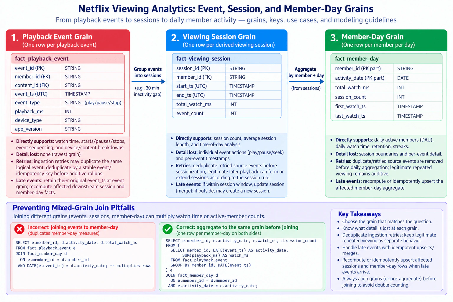
Choose event, session, and member-day grains for Netflix viewing analytics. diagram
How to Explain It in an Interview

Start by declaring the grain of every fact.

  1. Playback event fact — one row per playback event The primary key is event_id. The fact also carries member_id, content_id, event_ts in UTC, event_type, playback_ms, device_type, and app_version. This is the rawest grain, so it preserves event sequencing and individual play, pause, and stop actions. It directly supports watch-time calculations, starts, pauses, stops, event sequencing, and device or content breakdowns. No event-level detail is intentionally lost.

Ingestion retries may deliver the same logical event more than once. Deduplicate those rows using a stable event or idempotency key before additive rollups. A legitimate repeated viewing action remains a separate event. A late event keeps its original event_ts; after it arrives, downstream session and member-day facts that depend on it must be recomputed or updated.

  1. Viewing session fact — one row per derived viewing session The primary key is session_id, with member_id as a foreign key. The shown session fact contains start_ts, end_ts, total_watch_ms, and event_count. Events are grouped into sessions using a declared sessionization rule, such as the diagram's example of a 30-minute inactivity gap.

This grain directly supports session count, average session length, and time-of-day analysis. The tradeoff is that individual event actions and per-event timestamps are no longer available from the session row. Retried source events must therefore be deduplicated before sessionization. Legitimate later playback can extend or form a session according to the session rule. A late event within the session window can update the affected session; an event outside that boundary can create a new session.

  1. Member-day fact — one row per member per activity date Its composite primary key is (member_id, activity_date). The shown measures are total_watch_ms, session_count, first_watch_ts, and last_watch_ts. This grain directly supports daily active members, daily watch time, retention-style analysis across days, and streak calculations. It intentionally loses session boundaries and individual event detail.

Duplicate or retried source events are removed before daily aggregation, while legitimate repeated viewing remains additive. When a late event changes a contributing session or event set, recompute or idempotently upsert the affected member-day row.

Prevent mixed-grain fan-out The major failure case is joining the event fact directly to the member-day fact on member_id and date and then summing daily measures. If a member has many events that day, the one member-day row repeats for every matching event, so total_watch_ms, session_count, or an active-member measure can be multiplied.

The safe pattern is to aggregate the finer-grained fact to the target grain first. For example, reduce playback events to one row per (member_id, activity_date), then join that result to the one-row-per-member-day fact on the same key. The same rule applies when mixing event, session, and member-day facts: choose the metric's required grain, aggregate each contributing fact to that grain, and only then join.

The practical tradeoff is simple: event grain gives maximum flexibility but more rows and more downstream logic; session grain is convenient for session behavior but loses event detail; member-day grain is compact and efficient for daily metrics but cannot answer event- or session-level questions by itself.

Technical Approach
  1. Declare the three grains explicitly: one row per playback event, one row per derived viewing session, and one row per member per activity date.
  2. Keep event_id as the playback-event primary key and retain the detailed event attributes and playback contribution at that grain.
  3. Deduplicate ingestion retries by a stable event or idempotency key before sessionization or additive aggregation.
  4. Group deduplicated events into sessions using the agreed session boundary rule; store one session_id row with member_id, start and end timestamps, total watch time, and event count.
  5. Aggregate sessions to (member_id, activity_date) for the member-day fact and store daily watch time, session count, first watch timestamp, and last watch timestamp.
  6. When late events arrive, keep their original event time and recompute or idempotently update affected downstream session and member-day rows.
  7. Before joining facts at different grains, aggregate every contributing side to the same target grain and then join on the complete grain key.
Practical Insights

The event fact has the highest data volume because it keeps every playback action, so it costs the most storage and requires more rows to scan. The session fact is smaller because many events become one session row. The member-day fact is smaller again because many sessions become one daily row per member. These summaries make common daily and session queries simpler and cheaper, but they require transformation logic and late-data maintenance. Deduplication and recomputation also add processing cost. The main maintenance rule is to define each grain clearly and keep metric logic consistent so retries and joins cannot silently inflate totals.

Why Interviewers Ask This

The interviewer is testing whether the candidate can declare a fact-table grain before choosing keys and measures, understand what detail is lost during aggregation, handle duplicate retries and late-arriving events safely, and prevent fan-out when facts at different grains are joined. It also tests whether the candidate can choose the smallest useful grain for a metric instead of forcing every analytical question onto one table.

Common interview mistakes

Common mistakes are declaring no explicit grain; treating ingestion retries as legitimate additional viewing; deduplicating real repeated viewing along with retries; putting event-level attributes into a session or member-day fact after that detail has been discarded; assuming a session has one content or device when the session rule does not guarantee it; ignoring the time-zone definition of a member day; failing to recompute summaries for late events; and directly joining event, session, and member-day facts before aggregation. The last mistake causes fan-out, where higher-grain measures such as daily watch time or session count repeat across multiple lower-grain rows and become inflated.

Interview tip

Lead with the grain decision. Say what one row means for each fact, name its key and useful measures, then explain what detail aggregation removes. Finish with the two correctness rules interviewers care about most: deduplicate ingestion retries before additive rollups, and aggregate mixed-grain facts to the same target grain before joining.

Interviewer may ask next
How would you handle a playback event that arrives late after its session and member-day rows have already been created?

Keep the event at event grain with its original event_ts. Deduplicate it first using the stable event or idempotency key. Then determine which derived session the event belongs to under the session boundary rule. Recompute or idempotently update that affected session. Finally, recompute or upsert the corresponding (member_id, activity_date) member-day row so total_watch_ms, session_count, first_watch_ts, and last_watch_ts reflect the corrected inputs. The update must be repeatable so processing the same late event again does not double count it.

Why is joining the playback-event fact directly to the member-day fact dangerous, and how would you make the join safe?

The event fact can have many rows for one member-day, while the member-day fact has exactly one row for that member and date. A direct join therefore repeats the member-day row once for every matching event. Summing total_watch_ms, session_count, or an active-member value after that join can multiply the metric. First aggregate the event fact to one row per (member_id, activity_date). Then join the two one-row-per-member-day results on both key columns. More generally, aggregate every fact to a common target grain before combining additive measures.

3. Model daily Netflix content engagement for every title and country.Data ModelingMediumNetflix

Question Details

Declare source-event and published-aggregate grains for title-country-day metrics such as viewers, starts, completions, and watch duration. Specify content and geography keys, timezone policy, late-arrival and correction versions, title availability history, and how multi-device activity and repeated plays are counted without mixing distinct-member and event measures.

Short Interview Answer (30-60 seconds)

I would keep one source row per playback or engagement event, resolve its title, country, reporting date, and historical availability, then aggregate to title-country-day. Viewers are distinct members; starts, completions, and watch time are event measures. Corrections replace older event versions and republish the affected day with a higher correction version.

Detailed Explanation

The goal is to count how people use each Netflix title in each country every day without counting the same correction twice or treating every activity as a new person. Each activity is stored separately with its time, title, member, device, country, and amount watched. The day is chosen using the reporting time rule for that country. Historical title availability is checked for that day. If an earlier activity is corrected, its newer copy replaces the old one. Daily results can then be republished while earlier published versions remain identifiable.

Useful Questions to Ask the Interviewer
  1. Should the reporting day use one business-defined reporting timezone per country metric, even for countries that span multiple civil timezones?
  2. Which event types qualify a member as a viewer?
  3. Is a completion represented by a dedicated completion event, as shown in the model?
  4. Should historical correction versions remain queryable, or should consumers only see the latest version?
  5. Is title-country availability evaluated using the derived reporting_date, as shown in the diagram?
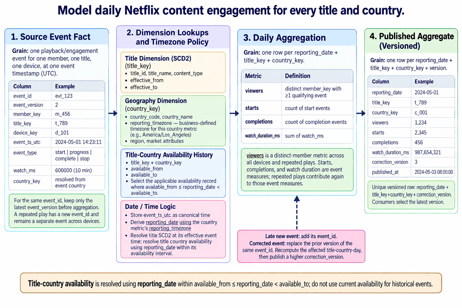
Model daily Netflix content engagement for every title and country. diagram
How to Explain It in an Interview

Start by declaring the source grain: one playback or engagement event for one member, one title, one device, at one UTC event timestamp. Each source event has event_id as its event identity and event_version for corrections. member_key identifies the member, title_key identifies the content, device_key identifies the device, country_key is resolved from the event country, event_type describes activity such as start, progress, complete, or stop, and watch_ms stores the watch duration contributed by that event.

Before aggregation, deduplicate corrected events by event_id and keep only the latest event_version. A repeated play is different from a correction: it has a new event_id, so it remains a separate event even when the same member watches the same title again or uses another device.

Next resolve the dimensions. The Title Dimension is an SCD2, or slowly changing dimension type 2. It uses title_key and keeps title_id, title_name, content_type, effective_from, and effective_to. Resolve the applicable title version at the event's effective time so historical events do not use only the current title record.

The Geography Dimension uses country_key and contains country_code, country_name, region or market attributes, and reporting_timezone. reporting_timezone is a business-defined timezone for the country metric; it does not mean every country has only one civil timezone. Keep event_ts_utc as the canonical timestamp, then derive reporting_date by converting that timestamp using the selected reporting_timezone.

Keep Title-Country Availability History separately using title_key + country_key, available_from, and available_to. Select the applicable availability record where available_from <= reporting_date < available_to. This prevents current title availability from being applied incorrectly to historical engagement.

After those lookups, aggregate to one logical row per reporting_date + title_key + country_key. Keep the metric semantics separate. viewers is a distinct-member measure: count each member_key once when that member has at least one qualifying event for that title-country-day, even if the member uses several devices or generates several events. starts is the count of start events. completions is the count of completion events. watch_duration_ms is the sum of watch_ms. Repeated plays can therefore contribute additional starts, completions, and watch duration, but they do not create additional viewer counts for the same member within the same title-country-day.

For publication, retain correction versions. The published grain is one row per reporting_date + title_key + country_key + correction_version. The published row contains the daily engagement metrics and published_at. Consumers select the latest correction_version for each reporting_date, title_key, and country_key.

Late and corrected source data require targeted reprocessing. A late new event contributes its new event_id. A corrected event replaces the prior version of the same event_id by using the latest event_version. Recompute the affected title-country-day and publish a higher correction_version. This prevents double-counting corrected events while keeping published history identifiable.

The main tradeoff is that historical dimensions, availability history, event versions, and published correction versions require more storage and processing than simply overwriting current rows. In return, the model provides reproducible historical reporting, controlled correction handling, and clean separation between distinct-member viewers and event-level engagement measures.

Technical Approach
  1. Ingest each playback or engagement record at the source-event grain with event_id and event_version.
  2. For each event_id, keep only the latest event_version before aggregation.
  3. Resolve country_key from the event country.
  4. Use the Geography Dimension's business-defined reporting_timezone to convert event_ts_utc into reporting_date.
  5. Resolve the applicable Title Dimension SCD2 record at the event's effective time.
  6. Resolve Title-Country Availability History where available_from <= reporting_date < available_to.
  7. Group qualifying events by reporting_date, title_key, and country_key.
  8. Compute viewers as distinct member_key, starts as the count of start events, completions as the count of completion events, and watch_duration_ms as the sum of watch_ms.
  9. For a late new event or corrected event, recompute only the affected title-country-day and publish a row with a higher correction_version.
  10. Have consumers select the latest correction_version for each title-country-day.
Practical Insights

Processing cost grows mainly with the number of source events because each event must be checked for its latest version, assigned a reporting date, matched to historical title and availability records, and included in an aggregation. Distinct viewers usually need more working memory than simple event counts because member identities must be tracked inside each title-country-day group. Historical dimension rows and correction versions use extra storage. Late-event handling adds operational cost, but recomputing only affected title-country-day results avoids rebuilding all historical data.

Why Interviewers Ask This

This question tests whether the candidate can define source and aggregate grains precisely, separate distinct-member metrics from event metrics, model historical title and availability data, apply a stable reporting-timezone policy, and handle late-arriving or corrected events without double-counting. It also tests whether the candidate can design versioned published aggregates with clear consumer semantics.

Common interview mistakes

Common mistakes are leaving the source grain vague; counting events as viewers instead of distinct members; counting the same member multiple times because activity came from several devices; treating a repeated play as a correction instead of a new event; aggregating multiple event_version rows for the same event_id; deriving country identity from timezone instead of resolving country from the event; using UTC date instead of the business-defined reporting timezone; resolving title SCD2 history to the current title record instead of the effective historical version; using current title availability for historical events; combining title SCD2 history and title-country availability history into one concept; overwriting published aggregates without correction_version; and summing multiple published correction versions when consumers need the latest title-country-day result.

Interview tip

State the two grains first. Then separate distinct-member viewers from event measures, explain reporting-date and historical availability resolution, and finish with event-version deduplication plus correction-version publication. That order makes the model easy to explain and defend.

Interviewer may ask next
How would you handle the same member watching the same title several times on different devices in one day?

Treat each repeated play as a separate source event with its own event_id, regardless of device. Those events can each contribute starts, completions, and watch_ms. For viewers, count distinct member_key within the title-country-day, so the member contributes only one viewer even if they generate many events across several devices.

What happens when a playback event arrives late or an existing event is corrected after the daily aggregate was published?

A late new event is added using its new event_id. A corrected event uses the same event_id with a newer event_version, so the earlier version is replaced before aggregation. Recompute the affected reporting_date + title_key + country_key result and publish it with a higher correction_version. Historical published versions remain identifiable, while consumers select the latest correction_version.

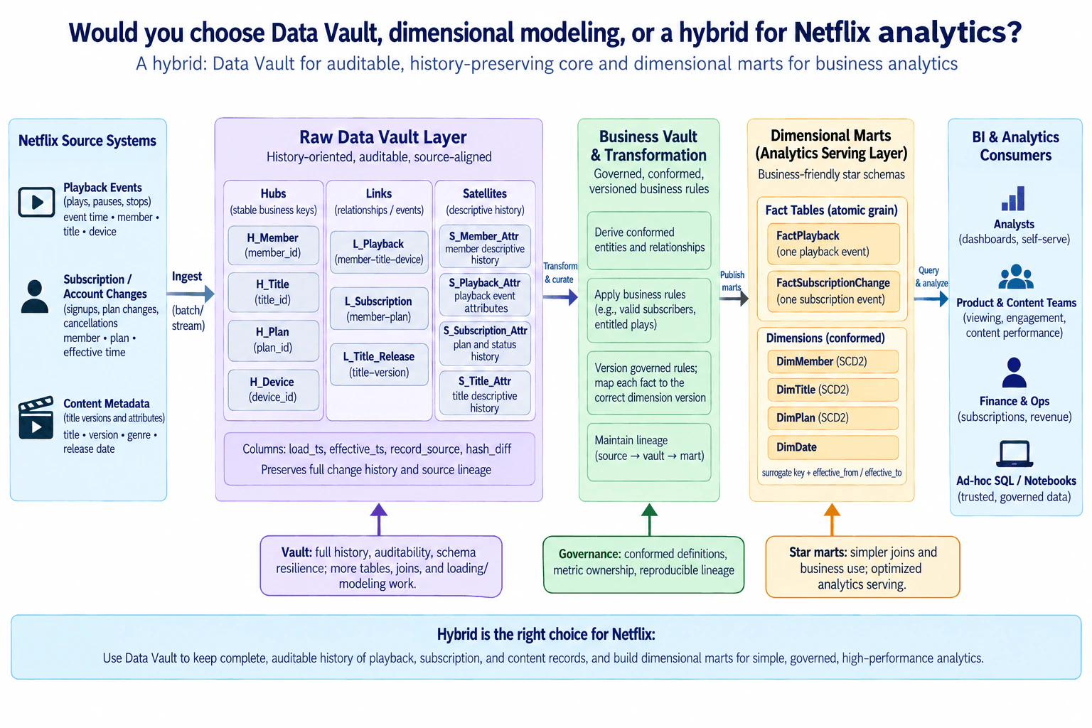
4. Would you choose Data Vault, dimensional modeling, or a hybrid for Netflix analytics?Data ModelingHardNetflix

Question Details

Compare source-history preservation, auditability, schema volatility, business usability, join complexity, loading effort, governance, and serving performance. Define which Netflix playback, subscription, or content records remain in history-oriented structures and which become dimensional marts, including lineage and version boundaries between the two layers.

Short Interview Answer (30-60 seconds)

I would use a hybrid: Data Vault for complete, auditable playback, subscription, and content history, then governed dimensional marts for business analytics. The vault absorbs source changes and preserves lineage, while star schemas give analysts simpler joins, clear grains, conformed dimensions, and efficient analytical serving.

Detailed Explanation

Netflix needs two things at the same time. It must keep a trustworthy record of how viewing, memberships, plans, and titles changed over time, and it must also make that information easy for people to explore. One structure is better at keeping detailed history when incoming data changes. Another is better for simple reports and analysis. I would therefore keep the detailed source history first, apply shared business rules in one controlled place, and then publish simpler business-facing tables for analysts, product and content teams, finance and operations, and trusted ad-hoc analysis.

Useful Questions to Ask the Interviewer
  1. Must every source change be retained for replay, auditing, or backfills?
  2. How often do playback, subscription, and content source schemas change?
  3. Which analytics require point-in-time historical correctness rather than only current attributes?
  4. What latency is required between source ingestion and dimensional-mart availability?
  5. Who owns conformed definitions for members, titles, plans, and shared business metrics?
  6. Do analysts, product and content teams, finance and operations, and ad-hoc SQL or notebook users need different serving models or freshness guarantees?
Would you choose Data Vault, dimensional modeling, or a hybrid for Netflix analytics? diagram
How to Explain It in an Interview
1. Practical decision: choose a hybrid

I would not use Data Vault alone as the normal business-consumption model, and I would not use dimensional marts as the only historical store. I would use the same hybrid flow shown in the diagram:

Netflix source systems → Raw Data Vault Layer → Business Vault & Transformation → Dimensional Marts → BI & Analytics Consumers.

Playback events, subscription or account changes, and content metadata can arrive through batch or streaming ingestion. The Raw Data Vault is the history-oriented, auditable, source-aligned layer. The dimensional marts are the business-friendly analytics-serving layer.

2. What remains in the Raw Data Vault

The Raw Data Vault preserves source-aligned history for playback, subscription, and content records.

Stable business keys are represented by Hubs: H_Member(member_id), H_Title(title_id), H_Plan(plan_id), and H_Device(device_id).

Links represent relationships or events: L_Playback(member-title-device), L_Subscription(member-plan), and L_Title_Release(title-version).

Satellites preserve descriptive history: S_Member_Attr for member descriptive history, S_Playback_Attr for playback event attributes, S_Subscription_Attr for plan and status history, and S_Title_Attr for title descriptive history.

The diagram also keeps technical lineage and history fields such as load_ts, effective_ts, record_source, and hash_diff. Together, these structures preserve change history and source lineage so downstream models can be reconstructed when rules or source structures change.

3. Why Data Vault fits the history layer

Data Vault is useful when source schemas are volatile because descriptive changes can be isolated in satellites instead of forcing one large business-facing schema to absorb every source change. It also supports auditability because business keys, relationships, descriptive history, load timing, effective timing, and record source remain traceable.

The tradeoff is complexity. A vault usually has more tables, more joins, and more loading and modeling work than a star schema. That is why I would not make Raw Data Vault structures the default interface for analysts.

4. What happens in Business Vault & Transformation

This layer turns source-aligned history into governed business meaning. It derives conformed entities and relationships, applies business rules such as valid-subscriber and entitled-play logic, manages versioned rules, maps each fact to the correct dimension version, and maintains lineage from source to vault to mart.

This is also the governance boundary. Shared definitions, metric ownership, and reproducible lineage should be controlled here instead of being reimplemented independently in dashboards or notebooks.

5. What becomes dimensional marts

The dimensional layer contains business-friendly star schemas.

FactPlayback has the declared grain of one playback event.

FactSubscriptionChange has the declared grain of one subscription event.

Conformed dimensions include DimMember, DimTitle, DimPlan, and DimDate. DimMember, DimTitle, and DimPlan use Slowly Changing Dimension Type 2 when historical attribute versions must be retained.

A Type 2 dimension creates a new version row instead of overwriting the previous historical row. The dimensional layer therefore uses a surrogate key plus effective_from and effective_to boundaries to identify each version.

6. Version boundary between the vault and marts

Natural business identifiers such as member_id, title_id, and plan_id identify business entities in the vault. In the dimensional layer, Type 2 rows use surrogate keys so multiple historical versions of the same business entity can coexist.

When publishing a playback or subscription fact, the transformation resolves the natural business key together with the fact's effective time to the dimension row whose version was valid at that time. The fact stores that dimension version's surrogate key.

Conceptually, the lookup boundary is effective_from <= fact_time and fact_time < effective_to when the implementation uses a half-open validity interval. The exact representation of an open current row is a warehouse-modeling choice and should be defined consistently.

This prevents an old playback or subscription event from being described using a newer member, title, or plan version.

7. Compare the tradeoffs directly

Source-history preservation: Data Vault is stronger because playback, subscription, and content changes remain in history-oriented structures instead of being reduced to only the current business view.

Auditability: Data Vault is stronger because source lineage and historical versions remain traceable through fields such as record_source, load_ts, and effective_ts.

Schema volatility: Data Vault is better suited to changing source structures because descriptive history can evolve in satellites. Published dimensional marts need more controlled changes because they are business-facing contracts.

Business usability: Dimensional modeling is stronger. Fact and dimension structures are easier for analysts and business teams to understand.

Join complexity: Data Vault requires more joins across hubs, links, and satellites. Star marts provide simpler fact-to-dimension query paths.

Loading effort: The hybrid requires more engineering because data is ingested into the vault, transformed through governed rules, and then published into marts. That extra work buys historical traceability and a clean serving boundary.

Governance: The Business Vault and transformation layer provide a controlled place for conformed definitions, versioned business rules, metric ownership, and reproducible lineage.

Serving performance: Dimensional marts are the preferred analytics-serving layer because they reduce logical join complexity and can be physically optimized for analytical workloads. The logical star schema alone does not guarantee a specific speedup; actual performance still depends on the warehouse engine, data volume, partitioning or clustering, statistics, caching, and query patterns.

8. Consumer boundary

Analysts use the dimensional marts for dashboards and self-service analysis. Product and content teams use them for viewing, engagement, and content-performance analysis. Finance and operations use them for subscription and revenue-oriented analysis. Ad-hoc SQL and notebooks should query trusted, governed data rather than rebuilding business rules independently from raw vault structures.

9. Final recommendation

The hybrid creates a clear separation of responsibilities. Data Vault protects complete source history, auditability, lineage, and resilience to schema change. Business Vault & Transformation owns governed entities, business rules, lineage, and version mapping. Dimensional marts expose atomic playback and subscription facts with conformed member, title, plan, and date dimensions for simple analytical consumption.

For the playback, subscription, and content records in this question, that balance is stronger than choosing either Data Vault or dimensional modeling alone.

Technical Approach
  1. Identify the source domains: playback events, subscription/account changes, and content metadata.
  2. Ingest them through batch or streaming pipelines into the Raw Data Vault.
  3. Store stable business keys in H_Member, H_Title, H_Plan, and H_Device.
  4. Store relationships or events in L_Playback, L_Subscription, and L_Title_Release.
  5. Preserve descriptive history in the member, playback, subscription, and title satellites together with load_ts, effective_ts, record_source, and hash_diff.
  6. In Business Vault & Transformation, derive conformed entities, apply governed business rules, manage rule versions, and maintain source-to-vault-to-mart lineage.
  7. Declare dimensional fact grains explicitly: one playback event for FactPlayback and one subscription event for FactSubscriptionChange.
  8. Build conformed DimMember, DimTitle, DimPlan, and DimDate dimensions.
  9. Use SCD Type 2 for member, title, and plan history where historical versions matter.
  10. Resolve every historical fact to the surrogate key whose effective_from/effective_to interval contains that fact's effective time.
  11. Publish the marts for dashboards, product/content analysis, finance/operations analysis, and governed ad-hoc SQL or notebooks.
Practical Insights

The hybrid costs more to build and maintain than a single modeling approach. The vault creates more tables and joins, so ingestion, loading, testing, lineage tracking, and developer effort increase. Type 2 dimensions also keep multiple historical versions, which increases storage. Dimensional marts add another transformation and serving layer. In return, source changes are easier to absorb without losing history, audits and backfills are safer, business rules are governed centrally, and analysts work with simpler star-schema joins. Query performance still depends on the physical warehouse design and workload, not only on the logical modeling style.

Why Interviewers Ask This

This question tests whether the candidate can separate historical integration needs from analytics-serving needs. A strong answer should compare auditability, source-history preservation, schema volatility, loading effort, join complexity, governance, business usability, lineage, and serving performance. It also tests whether the candidate can define clear fact grains and version boundaries when moving playback, subscription, and content data from a history-oriented model into dimensional marts.

Common interview mistakes

Common mistakes are using Data Vault directly as the default analyst-facing model, keeping only dimensional marts and losing source-aligned history, failing to declare fact grain, confusing natural business keys with dimensional surrogate keys, using SCD2 without effective_from/effective_to boundaries, mapping historical facts to the latest dimension version instead of the version valid at the fact time, allowing dashboards to redefine governed business rules independently, and claiming that dimensional modeling automatically guarantees fast queries without considering the physical warehouse and workload.

Interview tip

Lead with the hybrid decision. Then describe the boundary clearly: Raw Data Vault preserves source history and lineage, Business Vault & Transformation owns governed rules and version mapping, and dimensional marts serve consumers. State the two fact grains and explain how fact time resolves to the correct SCD2 surrogate-key version. That shows both modeling depth and practical analytical judgment.

Interviewer may ask next
How would you map a historical playback event to the correct DimMember or DimTitle Type 2 row?

Use the natural business key from the vault together with the playback event's effective time. Resolve the dimension row for that business key whose validity interval contains the event time, for example effective_from <= event_time and event_time < effective_to when using a half-open interval. Store that row's surrogate key in FactPlayback. This keeps historical playback tied to the member or title version that was valid when the event occurred rather than to the latest version.

When would you choose only dimensional modeling instead of the hybrid?

I would consider dimensional-only modeling when source structures are stable, detailed source-history reconstruction is not required, auditability and lineage requirements are modest, and the main goal is straightforward analytical serving. It reduces modeling and loading effort. For this question, however, explicit requirements around playback, subscription, and content history, auditability, schema volatility, lineage, and version boundaries make the hybrid more appropriate.

5. Design a daily incremental Spark pipeline for Netflix member watch time with seven-day-late events.Data PipelinesEasyNetflix

Question Details

Start from raw playback events partitioned by event_date and publish member-level daily watch-time output queried through Trino or Presto. Define a rolling seven-day reprocessing window, deduplication key, partition overwrite or versioned publish, checkpoints, late-volume watermark, and the validation proving reruns incorporate delayed records without changing unaffected partitions.

Short Interview Answer (30-60 seconds)

I would run a daily Spark batch that reprocesses event_date partitions D - 7 through D. Spark deduplicates playback_event_id, aggregates watch_seconds by member_id and event_date, and overwrites only those recent output partitions. A checkpoint records the successful processing date and published commit. Reruns must produce the same deduplicated result, while checks confirm older partitions remain unchanged. The trade-off is extra repeated processing in exchange for reliable handling of events arriving up to seven days late.

Detailed Explanation

The goal is to calculate how much each Netflix member watched on each day, even when some playback records show up several days after the viewing happened. Instead of updating only the newest day, every daily run looks back far enough to include records that arrived late. It recalculates only that recent period, removes repeated playback records, and leaves older results alone. The design also records the last completed run, checks that repeating a run gives the same answer, and raises attention when records arrive too late for the normal correction period.

Useful Questions to Ask the Interviewer
  1. Does "seven days late" mean an event for D - 7 must still be included in the run for processing date D?
  2. Is playback_event_id guaranteed to uniquely identify one playback event across reruns?
  3. Can the destination safely replace individual event_date partitions, or should publication use a versioned commit?
  4. What late-event count or rate should trigger the late-volume alert?
Design a daily incremental Spark pipeline for Netflix member watch time with seven-day-late events. diagram
How to Explain It in an Interview
1. Define the raw playback-event contract

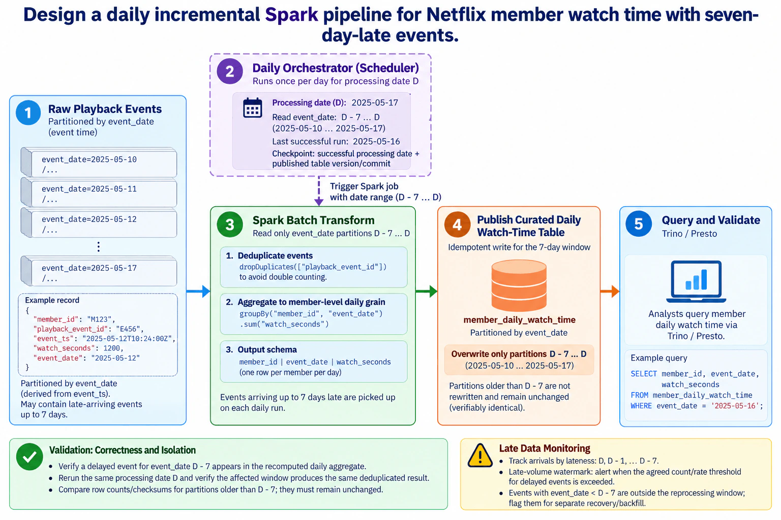
I would start with the Raw Playback Events dataset. It is partitioned by event_date, and the diagram shows event_date being derived from event_ts. The visible record fields are member_id, playback_event_id, event_ts, watch_seconds, and event_date. The important distinction is that event_date represents when the playback happened, while processing date D represents when the daily batch runs. Because an event may arrive as much as seven full days late, the run for D must still be able to include an event whose event_date is D - 7.

2. Trigger one daily rolling reprocessing run

The Daily Orchestrator runs once per day for processing date D and triggers the Spark job with the date range D - 7 through D. This is an inclusive range, so the example for D = 2025-05-17 reads event_date partitions 2025-05-10 through 2025-05-17. The scheduler owns the control flow; Spark owns the data transformation. The scheduler records the last successful processing date and a checkpoint containing the successful processing date plus the published table version or commit. That checkpoint records completed progress and is separate from the member watch-time data itself.

3. Deduplicate and aggregate in Spark

Spark reads only the selected event_date partitions. It first removes duplicates using playback_event_id as the deduplication key, which prevents replayed copies of the same playback event from adding watch time more than once. Spark then groups by member_id and event_date and sums watch_seconds. The destination grain is exactly one row per member per day, represented as member_id, event_date, and watch_seconds. Recomputing the complete recent range means late records inside the supported boundary are naturally incorporated into the correct member-day aggregate.

4. Publish only the affected partitions

The curated output is member_daily_watch_time, partitioned by event_date. Each run overwrites only partitions D - 7 through D. For the example run, that means 2025-05-10 through 2025-05-17. Partitions older than D - 7 are not rewritten. This creates the idempotent publication behavior shown in the diagram: rerunning the same processing date against the same source records should produce the same deduplicated member-day values instead of adding another copy of the watch time. Trino or Presto then queries the published member_daily_watch_time table.

5. Prove correctness with rerun and isolation checks

I would not treat Spark job success as proof that the data is correct. First, verify that a delayed event for event_date D - 7 appears in the recomputed daily aggregate. Second, rerun the same processing date D and verify that the affected range produces the same deduplicated result. Third, compare row counts or checksums for partitions older than D - 7 and confirm they remain unchanged. Together, these checks prove that delayed records are incorporated, duplicate records are not double counted, and unrelated historical partitions are isolated from the normal daily rerun.

6. Monitor late data and handle records outside the window

Late Data Monitoring is separate from the main business-data path. Track arrival volume by lateness bucket: D, D - 1, through D - 7. Raise an alert when the agreed count or rate of delayed events exceeds its threshold. If an event has event_date earlier than D - 7, it is outside the normal reprocessing range and should be flagged for a separate recovery or backfill. The benefit of this design is simple, deterministic correction of recent data. The downside is repeated Spark reads, aggregation, and writes for the recent partitions on every daily run.

Technical Approach
  1. Run the workflow once per day for processing date D.
  2. Select raw event_date partitions from D - 7 through D inclusive.
  3. Read those partitions with Spark.
  4. Deduplicate events using playback_event_id.
  5. Group by member_id and event_date and sum watch_seconds.
  6. Produce one row per member_id and event_date.
  7. Overwrite only member_daily_watch_time partitions D - 7 through D.
  8. Record the successful processing date and the published table version or commit in the checkpoint.
  9. Verify that a delayed D - 7 event appears in the recomputed aggregate.
  10. Rerun the same processing date and confirm the affected range produces the same deduplicated result.
  11. Compare row counts or checksums for partitions older than D - 7 and confirm they remain unchanged.
  12. Track late-arrival volume by lateness bucket and flag events older than D - 7 for separate recovery or backfill.
Practical Insights

The benefit is simple and predictable correctness. Each daily run processes only the recent event-date range from D - 7 through D instead of rebuilding all history. The downside is repeated compute and I/O because those recent partitions are read, deduplicated, aggregated, and written again every day. We accept this because it makes late-event correction and rerun behavior easy to reason about. Deduplication and grouping also require Spark shuffle work, so the cost grows with the amount of playback data in the selected range. A longer lateness boundary would capture more delayed records automatically but would increase repeated work. Events older than D - 7 stay outside the normal run and require a separate backfill rather than silently modifying historical partitions.

Why Interviewers Ask This

This question tests whether a candidate can keep a batch pipeline correct when records arrive late or are replayed. The interviewer wants to see good judgment around event time, processing time, partition selection, deduplication, idempotent reruns, checkpoints, safe publication, validation, and backfills. It also tests whether the candidate understands that successful execution alone does not prove data correctness and can explain the cost-versus-correctness trade-off of repeatedly processing recent partitions.

Common interview mistakes

Common mistakes are processing only partition D and therefore missing delayed events; confusing processing date with event_date; using the wrong aggregation grain; failing to deduplicate playback_event_id before summing watch_seconds; rewriting historical partitions outside D - 7 through D; advancing the success checkpoint before the intended publication is complete; assuming task success proves data correctness; claiming exactly-once behavior without support; allowing reruns to add watch time again; and silently ignoring events older than D - 7 instead of flagging them for a separate recovery or backfill.

Interview tip

Lead with the main correctness decision: every daily run reprocesses D - 7 through D. Then state the deduplication key, member-day grain, selective partition overwrite, checkpoint, and validation checks. Keep the scheduler's control flow separate from Spark's data transformation. Finish with the trade-off: repeated processing costs more, but it gives a simple and reliable way to correct seven-day-late data.

Interviewer may ask next
What would you change if playback events could arrive 30 days late instead of seven days?

I would change the lateness boundary while keeping the same basic pipeline. The Daily Orchestrator would trigger Spark with a wider date range, and Spark would re-read the required recent event_date partitions, still deduplicate by playback_event_id, and aggregate to one row per member_id and event_date. The curated member_daily_watch_time table would overwrite only that wider affected range, while older partitions would remain untouched.

Validation would move to the new boundary as well. I would verify that an event arriving at the maximum supported lateness appears in its recomputed daily aggregate, rerun the same processing date and confirm the deduplicated result is stable, and compare older partitions to prove they did not change. Late Data Monitoring would track the wider lateness range and flag anything beyond it for separate backfill.

The main downside is cost. A wider range means more source reads, Spark shuffle work, and output rewrites every day. If that became too expensive, I would discuss a more selective correction strategy without weakening the correctness requirement.

How would you recover if the Spark job failed after some recent output partitions had already been written?

I would first use the scheduler state and publication checkpoint to determine whether the intended run completed. A failed workflow must not record the new processing date and published commit as successfully completed if publication did not finish. I would then rerun the same processing date D so Spark rereads D - 7 through D, deduplicates playback_event_id, recomputes the member-day aggregates, and replaces the intended recent partitions again.

The rerun is safe at the business-result level because the transformation rebuilds the affected member-day values from the source records instead of adding another copy of previously calculated watch time. After recovery, I would repeat the diagram's validation: confirm delayed records are present, verify the repeated run produces the same deduplicated result, and compare row counts or checksums for partitions older than D - 7.

The downside is repeated compute and write work during recovery, but the source contract, member-day grain, Trino or Presto serving path, and late-data policy remain unchanged.

6. Make a Netflix viewing-session workflow idempotent and safe to backfill.Data PipelinesEasyNetflix

Question Details

Design the orchestration DAG for discovering raw playback partitions, validating inputs, deduplicating events, assigning thirty-minute-gap sessions, computing outputs, and publishing them. Include data-based dependencies, run parameters, retries, task-level checkpoints, isolated backfill output, atomic promotion, and checks showing that repeating a date produces the same session facts.

Short Interview Answer (30-60 seconds)

I would make each date a deterministic run. The DAG discovers the required raw playback partitions, validates and deduplicates events, orders each viewer's events by event time, applies the 30-minute session gap, and writes candidate session facts to isolated staging. Failed tasks retry with the same inputs and parameters. After count, uniqueness, and repeat-run checks pass, I atomically promote the staged result. The trade-off is extra staging and validation work in exchange for safer retries and backfills.

Detailed Explanation

The goal is to process a viewing date again without accidentally creating different results or changing the live result too early. For the requested date, the process first finds all required playback data. It checks that the input is complete and removes repeated records. It then groups each viewer's activity into sessions using a thirty-minute break rule. The new result stays separate from the currently visible result until checks pass. If the same date is processed again with the same accepted input, the final viewing sessions should be the same.

Useful Questions to Ask the Interviewer
  1. What stable event identity should be used to recognize duplicate playback events?
  2. Are all required raw playback partitions expected to exist before a date can run, or can some arrive later?
  3. What storage mechanism provides the atomic promotion from validated staging to published session facts?
Make a Netflix viewing-session workflow idempotent and safe to backfill. diagram
How to Explain It in an Interview
1. Start with the run parameters and DAG

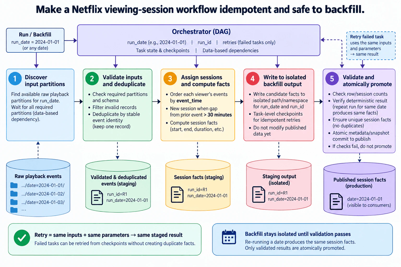
I would make run_date the business input for the date being processed and keep a run_id for the specific execution. The Orchestrator (DAG) owns task state, task-level checkpoints, data-based dependencies, and retries of failed tasks. A normal run and a backfill use the same processing logic. This matters because a retry must reuse the same inputs and parameters instead of silently changing the data being processed.

2. Discover the required input partitions

The first task is Discover input partitions. It finds the raw playback partitions needed for run_date. Downstream processing waits until all required partitions are available, so the dependency is based on data availability rather than only on a clock. If required input is missing, session processing should not proceed. This prevents an apparently successful run from creating session facts from incomplete source data.

3. Validate and deduplicate the events

Next, Validate inputs and deduplicate checks the required partitions and schema, filters invalid records, and removes duplicates using the defined stable event identity while keeping one record. The same accepted source records must always produce the same deduplicated result. The deduplicated events are held in staging rather than treated as published business output. The exact event identity belongs to the source contract and should be supplied by the system design rather than invented in the pipeline.

4. Assign sessions and compute facts

The Assign sessions and compute facts task orders each viewer's events by event_time. A new session starts when the gap from the prior event is greater than 30 minutes. The task then computes session facts such as the session start, end, and duration. Deterministic ordering plus a fixed gap rule is important because the same deduplicated event set should create the same session boundaries every time the date is processed.

5. Write isolated backfill output

The candidate result is written to Staging output (isolated) using the run_date and run_id. Published data is not changed yet. Task-level checkpoints let a failed task retry with the same inputs and parameters. Isolation prevents a partial backfill from mixing with the production result. The key rule is that a failed retry or unfinished backfill may change staging state, but it must not make incomplete session facts visible to consumers.

6. Validate and atomically promote

The final task, Validate and atomically promote, checks row or session counts, verifies that session facts are unique, and confirms the deterministic result by repeating the same date and comparing the resulting facts. If checks fail, the staged result is not promoted. If they pass, an atomic metadata or snapshot-style commit makes the validated result the published session facts. The exact atomic mechanism depends on the storage system, which is not specified here.

This gives one clear invariant: the same accepted inputs and parameters produce the same staged result, and only a validated result can replace the published result.

Technical Approach
  1. Accept run_date and a run_id.
  2. Discover all required raw playback partitions for the date.
  3. Wait until the required partitions are available.
  4. Validate the required partitions and schema.
  5. Filter invalid records and deduplicate accepted events using the defined stable event identity.
  6. Order each viewer's events by event_time.
  7. Start a new session whenever the gap from the previous event is greater than 30 minutes.
  8. Compute deterministic session facts.
  9. Write candidate facts to isolated staging associated with run_date and run_id.
  10. Use task-level checkpoints so failed tasks can retry with the same inputs and parameters.
  11. Validate row or session counts, uniqueness, and repeat-run equivalence.
  12. If validation fails, leave published data unchanged.
  13. If validation passes, atomically promote the staged result to published session facts.
Practical Insights

The main processing cost comes from reading one date of events, deduplicating them, and ordering each viewer's events before finding 30-minute gaps. Ordering can be the most expensive processing step when a viewer has many events. The benefit is that deterministic ordering gives repeatable session boundaries. Isolated staging also uses extra storage because a candidate result exists before publication. The downside is more operational work for checkpoints, validation, and cleanup. Strong validation can delay publication because the result waits for checks. We accept this because exposing partial or duplicate session facts would be worse than a slightly slower backfill. Processing many historical dates also increases compute and temporary storage use, but each date can still follow the same correctness contract.

Why Interviewers Ask This

This question tests whether a Data Engineer can separate workflow execution from data correctness. The interviewer wants to see sound judgment around deterministic processing, duplicates, event ordering, retries, checkpoints, historical backfills, validation, and publication boundaries. A strong answer shows that rerunning work is not enough by itself: partial results must remain isolated, and processing the same date again should produce the same business facts before anything becomes visible to consumers.

Common interview mistakes

Common mistakes are writing a backfill directly into published production data, retrying tasks without keeping writes idempotent, sessionizing before ordering each viewer's events by event_time, inventing a deduplication key instead of using the defined stable event identity, treating task success as proof that the data is correct, mixing outputs from different run_id values, promoting partial results, or skipping the repeat-run comparison. Another mistake is treating a failed-task retry and a historical backfill as the same operation. They reuse the same deterministic logic, but a retry repeats failed work within a run while a backfill intentionally processes an earlier run_date.

Interview tip

Center the answer on one invariant: the same accepted inputs and parameters must produce the same session facts. Then trace the diagram in order: discover, validate and deduplicate, assign sessions, write isolated output, validate, and promote. Explicitly separate failed-task retries from historical backfills and emphasize that published data does not change until validation passes.

Interviewer may ask next
What would you change if a large historical backfill had to process many dates at once?

I would keep the same correctness contract for each date and increase concurrency only across independent dates. Each date would still have its own run_date, run_id, discovered raw partitions, task checkpoints, session calculation, and isolated staging output. The requirement that changes is throughput: we want many historical dates to finish faster without allowing their intermediate results to interfere with one another.

The Orchestrator (DAG) can run multiple dates concurrently, but every date still follows the same flow: discover, validate and deduplicate, assign sessions, stage, validate, and promote. A failure for one date should retry only the failed task for that run and should not invalidate already completed dates.

Correctness stays intact because each date uses deterministic event-time ordering and the same greater-than-30-minute gap rule. Each date is validated independently before promotion. The main downside is higher temporary compute, staging storage, and orchestration load. I would therefore bound concurrency rather than allowing every historical date to run at once.

What should happen if repeating the same date produces different session facts?

I would block promotion of the new staged result. When the accepted inputs and processing rules are unchanged, repeating the same date is expected to produce the same session facts. A mismatch therefore means either the accepted input changed or one of the processing steps is not deterministic. The affected boundary is the final Validate and atomically promote task.

I would compare the two staged results and trace backward through the run: confirm that both executions discovered the same required partitions, accepted the same records after validation, used the same stable event identity for deduplication, ordered each viewer's records by the same event_time values, and applied the same 30-minute-gap rule.

The currently published session facts remain unchanged because the new result is still isolated in staging. After the difference is understood and corrected, the date can be run and validated again. The downside is delayed publication, but that is intentional because unexplained differences should never be promoted automatically.

7. Build a near-real-time Netflix Continue Watching pipeline from playback-progress events.Data PipelinesMediumNetflix

Question Details

Maintain a current member-content resume position for personalization while writing complete analytical history. Define transport partitioning, state key, event ordering across devices, exactly-once or idempotent sink behavior, late progress and completion events, checkpoints, replay, current-state compaction, historical publication, and a freshness measure for updates.

Short Interview Answer (30-60 seconds)

I would stream playback-progress events through Kafka, partitioned by (member_id, content_id), and process them with keyed Flink state using event time. The processor accepts only valid newer state transitions, protects completion from older progress, and publishes the latest resume state to a compacted Kafka topic while appending full history separately. Checkpoints bind state to source offsets for recovery. I would use transactional output where supported, otherwise idempotent monotonic upserts. The trade-off is more state and coordination in return for fresh, correct cross-device results.

Detailed Explanation

The goal is to keep each member's Continue Watching position current even when the same title is watched on several devices. Updates may arrive late or in a different order from when they happened. The system must avoid letting an old message move a person's visible position backward or make a finished title active again. At the same time, it must keep every viewing update for later analysis. It also needs a safe way to recover after failures and a simple measurement showing how quickly new viewing activity becomes visible.

Useful Questions to Ask the Interviewer
  1. How fresh should the Continue Watching position be for members?
  2. How long are playback events retained for replay or backfill?
  3. Does a completion event always outrank older progress for the same member and content?
  4. Can the current-state Kafka sink participate in transactional checkpoint commits, or must writes be made idempotent?
Build a near-real-time Netflix Continue Watching pipeline from playback-progress events. diagram
How to Explain It in an Interview
1. Define the playback-progress contract

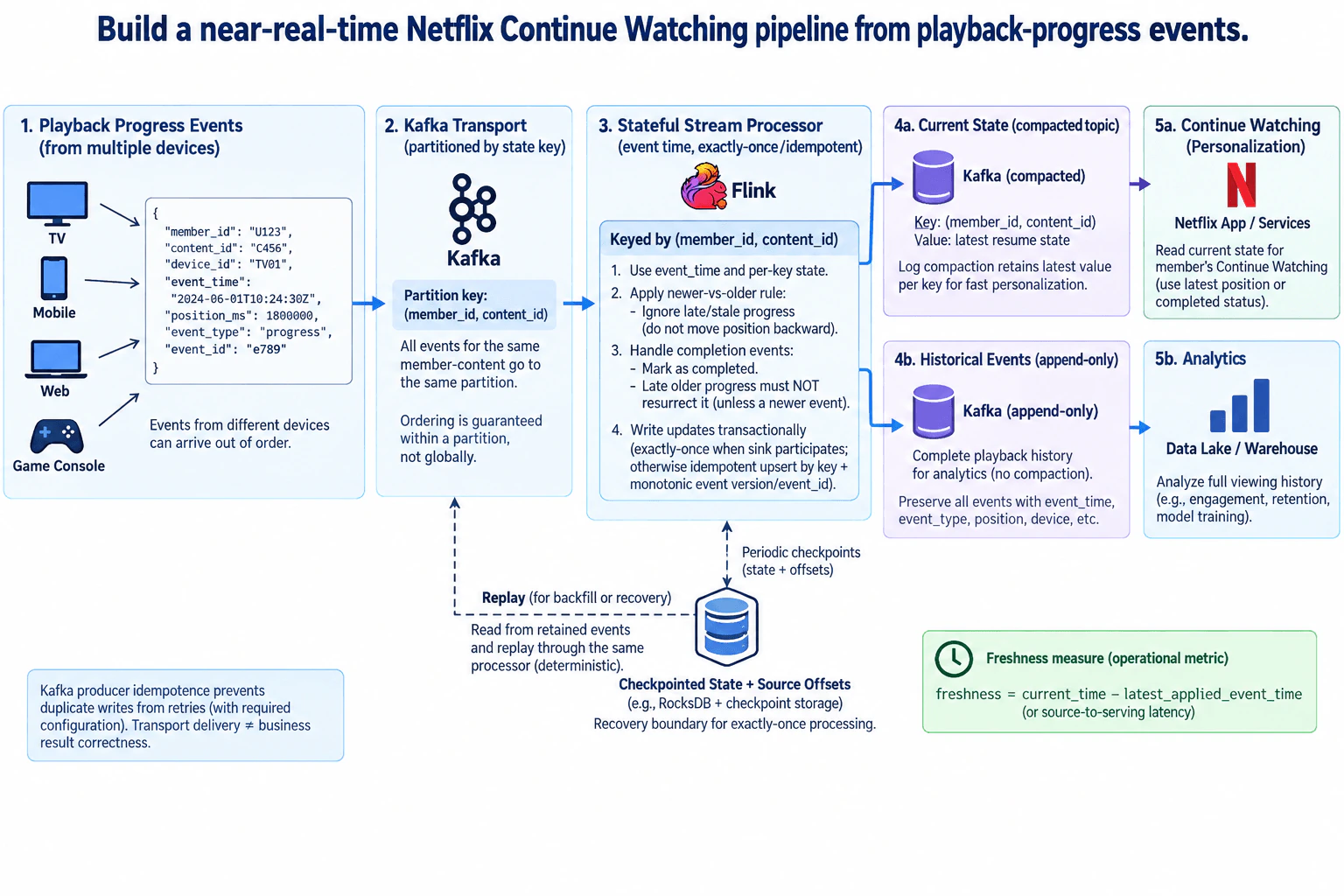
I would treat every playback update as an event from a TV, mobile device, web player, or game console. The visible contract contains member_id, content_id, device_id, event_time, position_ms, event_type, and event_id. The business grain for current state is one member-content pair. event_time tells us when playback happened on the source device, while processing time is when Flink handles the record. Events from different devices can arrive in a different order from when they occurred, so arrival order alone cannot determine the resume state.

2. Partition Kafka by the state key

I would publish the events to Kafka using (member_id, content_id) as the partition key. That sends events for one member-content pair to the same partition and gives the consumer one ordered transport sequence for that key. Kafka ordering is within a partition, not global across the topic. This partitioning also aligns transport with the downstream state key. Kafka producer idempotence can prevent duplicate broker writes caused by producer retries when configured correctly, but transport idempotence alone does not guarantee exactly-once business results.

3. Resolve cross-device ordering in keyed Flink state

Flink keys its state by the same (member_id, content_id) pair and applies event-time-aware state transitions. For progress events, the processor compares the incoming event with the newest accepted state and ignores late or stale progress that must not move the visible resume position backward. Completion is also stateful: a completion event marks the item complete, and an older progress event must not resurrect it. A genuinely newer event can change that state according to the same newer-versus-older rule. event_id or a monotonic event version can also support duplicate-safe state updates.

4. Publish current state and complete history separately

The processor has two output purposes. The latest resume state is written under the member-content key to a compacted Kafka topic. Log compaction retains the latest value for each key for the current-state path, so Netflix App / Services can read the latest position or completed status for Continue Watching. Separately, the processor publishes the complete playback history to an append-only, non-compacted Kafka topic. That path preserves events with fields such as event_time, event_type, position, and device before historical publication to the Data Lake / Warehouse for analytics such as engagement, retention, and model training.

5. Make business-result correctness explicit

If the Kafka sink participates in Flink's checkpoint-coordinated transaction, output can use an exactly-once processing boundary. If that transactional behavior is not available, I would make the current-state write idempotent: upsert by (member_id, content_id) and reject a write whose event version is older than the value already committed. This distinction matters because broker delivery semantics alone do not prove exactly-once business outcomes. A repeated record is safe only when processing it again leaves the same visible current state.

6. Recover with checkpoints and replay

Flink periodically checkpoints keyed state together with source offsets. As shown in the diagram, checkpointed state can use a state backend such as RocksDB plus durable checkpoint storage. After a failure, processing resumes from a consistent checkpoint instead of combining old state with unrelated newer source progress. For recovery or a controlled backfill, retained Kafka events are replayed through the same deterministic processor. The same stale-event rules and transactional or idempotent current-state writes make repeated processing safe. Replay of the append-only historical path must follow the defined backfill publication policy so historical duplicates are not introduced unintentionally.

7. Measure whether the result is actually near real time

I would track freshness separately from process health. A useful measure is current_time minus latest_applied_event_time for the current member-content state, or an equivalent source-to-serving latency. That directly answers whether a playback update has become visible quickly enough in Continue Watching. The main design trade-off is that keyed state, event-time comparison, checkpointing, and replay add storage, I/O, and coordination cost, but they prevent cross-device ordering errors while preserving both a fast current view and complete analytical history.

Technical Approach
  1. Receive playback-progress events containing member_id, content_id, device_id, event_time, position_ms, event_type, and event_id.
  2. Publish them to Kafka partitioned by (member_id, content_id).
  3. Key Flink state by the same pair.
  4. Compare each incoming event with the latest accepted event time or monotonic version for that key.
  5. Ignore stale progress and prevent older progress from reversing a newer completion state.
  6. Write current-state updates transactionally when the Kafka sink participates in checkpointing, otherwise use an idempotent monotonic upsert.
  7. Publish current state to a compacted Kafka topic and complete history to a separate append-only Kafka topic.
  8. Checkpoint keyed state and source offsets together.
  9. Replay retained events through the same processor for recovery or controlled backfill.
  10. Measure freshness from the latest applied event time to current time or serving visibility.
Practical Insights

The benefit is that partitioning and keyed state let each member-content pair be processed independently, so the pipeline can scale across Kafka partitions and Flink workers. The downside is that more partitions create coordination overhead, while long-lived keyed state consumes storage and increases checkpoint I/O. Event-time rules improve correctness when devices send late or out-of-order updates, but the processor must retain enough state to compare new and old events. Checkpoints make recovery deterministic, but very frequent checkpoints can hurt throughput. Replay is useful because the same logic can rebuild state, but it requires retained source history and extra compute. We accept these costs because an incorrect Continue Watching position is directly visible to the member, while analytical history also needs to remain complete.

Why Interviewers Ask This

This question tests whether a candidate can design a stateful streaming pipeline instead of simply moving events between systems. The important judgment is choosing the correct grain and partition key, handling events that arrive out of order across devices, separating transport delivery from business correctness, protecting completion state from stale progress, designing safe checkpoint and replay behavior, and serving fresh current state without losing complete analytical history.

Common interview mistakes

Common mistakes are partitioning only by member_id instead of the member-content state key; assuming Kafka provides global ordering; using arrival order instead of event-time-aware state for cross-device updates; allowing an older progress event to resurrect content after a newer completion; claiming Kafka producer idempotence creates exactly-once business results; recovering source offsets independently from processor state; writing only the current value and losing analytical history; compacting the historical stream; replaying through different logic from the live path; and measuring only broker or consumer health instead of end-to-end freshness of the applied Continue Watching state.

Interview tip

Lead with the state key and ordering problem. Explain that the hard part is not simply moving records through Kafka; it is producing one correct member-content state when several devices generate late and out-of-order events. Then separate current-state publication from historical publication, explain the checkpoint and replay boundary, and finish with the freshness metric.

Interviewer may ask next
What would you change if Continue Watching freshness had to be much lower while playback-event volume increased significantly?

I would keep the same Kafka-to-Flink architecture and scale the partitioned execution path without changing the correctness model. The requirement that changes is source-to-serving latency under higher load. Kafka would still partition by (member_id, content_id), because changing that key could break the single keyed-state owner model for each member-content pair. I would increase useful Kafka partition parallelism and Flink processing capacity while watching for hot keys, consumer lag, state size, checkpoint duration, and output capacity. The compacted current-state topic and append-only historical topic remain unchanged. I would also tune checkpoint frequency carefully: checkpoints must remain frequent enough for acceptable recovery, but making them too frequent can add I/O pressure and hurt freshness. Event-time comparison, completion handling, and transactional or idempotent publication remain unchanged, so correctness is preserved. Recovery still starts from a consistent checkpoint and source offsets. The main downside is higher compute, network, state, and checkpoint cost, with diminishing returns if Kafka partitions or downstream writes become the bottleneck.

How would you safely replay a long period of retained playback events without letting old progress corrupt the current Continue Watching state?

I would replay retained Kafka events through the same deterministic Flink logic used by the live stream, not through a separate transformation with different ordering rules. The changed requirement is historical reprocessing, while the member-content state contract stays the same. Each record is still keyed by (member_id, content_id), and the processor compares its event time or monotonic version with the newest accepted state. An older progress event therefore cannot move the visible position backward or resurrect a title after a newer completion. Current-state writes remain transactional when supported or idempotent monotonic upserts otherwise, so repeating an already processed event does not change the business result. Checkpointed state and source offsets provide the normal failure-recovery boundary during replay. I would verify the rebuilt current state by checking the latest accepted version for each key before considering the replay complete. The append-only historical path needs separate backfill publication rules because blindly replaying into it could create duplicate historical records. The downside is extra read, compute, state, checkpoint, and sink load during the replay.

8. Run a thirty-day, fifty-terabyte Netflix Keystone backfill while live processing stays fresh.NEWData PipelinesHardNetflix

Question Details

An upstream correction requires historical recomputation without pausing the live path. Separate backfill and real-time resources, pin source, schema, and code versions, define deterministic boundaries, write isolated Iceberg output, audit row counts and metric deltas, publish atomically with a WAP procedure, resume failed shards, merge late live data, and retain a rollback snapshot.

Short Interview Answer (30-60 seconds)

I would keep Keystone live processing on dedicated resources and run the 30-day, 50 TB recomputation as separately resourced deterministic shards using pinned source, schema, and code versions. Each shard writes only to isolated Iceberg staging. I would validate row counts and metric deltas, resume only failed shards, merge live data since the cutoff, create a validated WAP dynamic-overwrite snapshot, publish it atomically with publish_changes(wap_id), and retain the pre-publish snapshot for rollback. The trade-off is extra temporary capacity and storage for stronger isolation and recovery.

Detailed Explanation

The goal is to correct thirty days of old information without interrupting the information that is arriving now. I would treat the old work as a separate job with its own computing capacity, so it cannot slow the live path. I would freeze exactly what historical input and rules the job uses, split the large amount of work into repeatable pieces, check the completed result carefully, add anything new that arrived during the work, and expose the corrected result only after those checks pass. I would also keep the previous good result so we can quickly return to it if necessary.

Useful Questions to Ask the Interviewer
  1. What row-count expectations and metric-delta thresholds must the backfill satisfy before publication?
  2. What exact cutoff separates the historical backfill range from live data that must be reconciled before publication?
  3. How should the 30-day, 50 TB range be divided into resumable shards for the available backfill capacity?
Run a thirty-day, fifty-terabyte Netflix Keystone backfill while live processing stays fresh. diagram
How to Explain It in an Interview
1. Pin the historical inputs and boundaries

I would start by making the backfill deterministic. The diagram pins the source snapshot or version, the schema version, and the code version. It also fixes the historical range to thirty days; the visible example is 2024-01-01 through 2024-01-30. These pins prevent a retry from silently reading different source data or running different transformation logic. The live path continues to process new data, while the historical recomputation uses the fixed backfill boundary. This gives every shard a repeatable definition of what it must recompute.

2. Isolate live processing from the 50 TB backfill

The key production decision is resource isolation. Keystone real-time processing continues on separate, dedicated resources so live freshness does not depend on how quickly the historical work finishes. The backfill also receives separate, dedicated resources. The thirty-day, 50 TB range is divided into shards, and each shard performs deterministic historical recomputation. This limits the effect of a failure: one failed shard does not require restarting all thirty days. The main trade-off is extra temporary capacity, but that is preferable to allowing a huge historical workload to compete directly with the live path.

3. Write only to isolated Iceberg staging

Successful backfill shards write deterministic results to isolated Apache Iceberg staging. This output has no consumer visibility. That visibility boundary matters because a partially completed backfill must never appear to downstream readers as the final corrected dataset. Compute completion and publication are therefore separate events. The isolated staging area also lets failed shards be rerun without exposing intermediate results. The live Keystone path remains independent while historical output accumulates in staging.

4. Validate before publication

After the historical output is complete, the audit gate checks row counts against expectations and checks key metric deltas against accepted thresholds. A task finishing successfully is not enough to pass this gate. If a shard failed or produced incomplete output, retry or resume only that shard and run the checks again. If the data checks still fail, publication remains blocked; blindly repeating a technically successful shard would not prove correctness. Because the source, schema, code, and time boundaries are pinned, a resumed shard repeats the same intended computation.

5. Reconcile late live data and publish atomically

The live path keeps running throughout the backfill, so live data arriving since the backfill cutoff must be reconciled before the staged result becomes authoritative. The diagram sends that data into the final reconciliation step. After reconciliation and validation, the design creates one validated WAP dynamic-overwrite snapshot and publishes the staged change into the current Iceberg table state with publish_changes(wap_id). Iceberg's publication step creates a new table snapshot, so consumers do not see the isolated staging work incrementally; visibility changes at the table snapshot commit boundary.

6. Keep a recovery point

Before publication, I would retain the pre-publish Iceberg snapshot shown in the diagram. That snapshot is the rollback point. If the newly published result later proves unacceptable, the table can be rolled back to the retained pre-publish snapshot instead of requiring another full 50 TB recomputation before returning to the previous valid state. This design deliberately spends additional temporary storage and operational effort to gain deterministic reruns, live-path isolation, controlled publication, and a clear recovery boundary.

Technical Approach
  1. Pin the source snapshot or version, schema version, code version, and exact thirty-day backfill boundary.
  2. Keep Keystone real-time processing on separate dedicated resources.
  3. Split the 50 TB historical range into deterministic backfill shards running on separate resources.
  4. Write each completed shard only to isolated Iceberg staging with no consumer visibility.
  5. Audit expected row counts and required metric deltas.
  6. Retry or resume only failed or incomplete shards, then validate again.
  7. Keep publication blocked if validation still fails.
  8. Reconcile live data that arrived since the backfill cutoff into the staged result.
  9. Create the validated WAP dynamic-overwrite snapshot.
  10. Retain the pre-publish snapshot and atomically publish with publish_changes(wap_id).
  11. Roll back to the retained snapshot if the published result must be reversed.
Practical Insights

The benefit is strong isolation: a 50 TB historical job does not have to compete directly with the Keystone live path, and incomplete results stay hidden. Sharding also makes recovery cheaper because a failed piece can be repeated instead of rerunning all thirty days. The downside is extra compute capacity, temporary Iceberg storage, validation work, and a more careful publication process. Reconciliation adds another step because live data continues arriving while the historical job runs. Strong row-count and metric checks can delay publication, but that delay protects correctness. We accept these costs because keeping live processing fresh and preventing partially corrected historical data from becoming visible are more important than minimizing temporary resources or finishing the backfill as quickly as possible.

Why Interviewers Ask This

This question tests whether a candidate can run a very large historical correction without harming a continuously running production path. The interviewer wants to see clear separation of live and backfill resources, deterministic inputs, safe recovery from partial failures, validation before release, and careful handling of data that arrives while recomputation is running. It also tests whether the candidate understands that compute completion is not enough: publication needs a controlled visibility boundary and a usable rollback point.

Common interview mistakes

Common mistakes are running the 50 TB backfill on the same constrained resources as the live path, allowing source or code versions to change between shards, using vague historical boundaries, exposing partially completed Iceberg output, treating successful jobs as proof that the data is correct, rerunning all thirty days after one shard fails, forgetting live data that arrived after the historical cutoff, publishing before row-count and metric-delta checks pass, blindly retrying a deterministic shard when validation shows a real logic or data problem, or deleting the previous snapshot before the new result has proved safe.

Interview tip

Lead with the central decision: isolate live and backfill resources. Then walk left to right through pinned inputs, deterministic shards, hidden Iceberg staging, the audit gate, late-live reconciliation, the WAP dynamic-overwrite snapshot, publish_changes(wap_id), and rollback. Emphasize that compute success, data correctness, and consumer visibility are three different boundaries.

Interviewer may ask next
What would you change if several backfill shards fail after most of the 50 TB recomputation has already completed?

I would keep the successful shard outputs isolated and resume only the failed shards. The changed requirement is recovery efficiency: we need to recover partial compute without turning a local failure into another complete thirty-day run. The affected component is the backfill-shard path, not Keystone real-time processing. Because the source snapshot or version, schema version, code version, and deterministic range remain pinned, each failed shard can repeat the same intended work. Its replacement output still goes to isolated Iceberg staging, so no new consumer-visible path is introduced and partial recovery remains hidden. After the required shards succeed, I would run the same row-count and metric-delta audit again rather than assuming a retry is correct. If those checks fail for a genuine logic or data reason, publication stays blocked rather than looping retries. Only after validation would I reconcile live data since the cutoff and proceed to the WAP publication. The retained pre-publish snapshot remains the final recovery point. The downside is longer retention of temporary outputs and delayed publication.

What would you do if a large amount of live data arrives while the historical backfill is running?

I would keep the same architecture and make the final reconciliation boundary more important. The changed requirement is that more data now exists between the historical cutoff and publication. Keystone real-time processing must remain on its dedicated resources; I would not pause it or mix the 50 TB historical computation into that path. The historical shards would continue writing only to isolated Iceberg staging and would still pass the row-count and metric-delta audit. Before publication, all live data since the backfill cutoff would be merged into the staged result, preserving the same isolated visibility boundary rather than opening a new data path. After that reconciliation is complete and validated, I would create the validated WAP dynamic-overwrite snapshot and publish it with publish_changes(wap_id). The retained pre-publish snapshot remains available for rollback. The main downside is a larger and potentially longer reconciliation step, so final publication may be delayed, but live freshness and the existing recovery model remain unchanged.

9. Explain the S3, Iceberg, Trino, and Spark layers in Netflix’s lake architecture.Cloud Data PlatformsEasyNetflix

Question Details

Describe object durability, table metadata and snapshots, interactive SQL, and batch transformation responsibilities. Include catalog lookup, schema and partition evolution, concurrent readers and writers, atomic commits, file compaction, workload isolation, and the path from a raw object to a queryable published table.

Short Interview Answer (30-60 seconds)

I would separate durable S3 storage from Iceberg table state, Spark batch processing, and Trino interactive SQL. Spark transforms and compacts files, Iceberg publishes snapshots atomically, and Trino queries the published snapshot. The trade-off is efficient shared storage with separate compute and metadata complexity.

Detailed Explanation

Netflix data producers create application logs, events, ETL outputs, and partner data, while analysts, data scientists, product teams, and operational tools need stable queryable tables. A reusable lake platform avoids rebuilding storage, transformation, table publication, and SQL access for every dataset. The design separates durable objects in S3, logical table state in Iceberg, batch compute in Spark, and interactive query compute in Trino. It prioritizes durable storage, atomic table publication, schema and partition evolution, concurrent readers and writers, file maintenance, catalog-based discovery, and workload isolation without forcing all work onto one compute engine.

Useful Questions to Ask the Interviewer
  1. How fresh must published tables be for interactive Trino users?
  2. How much batch and interactive-query concurrency must the platform isolate?
  3. Which datasets require frequent schema or partition evolution?
  4. How aggressively should Spark compact small files versus preserving capacity for transformations?
  5. What recovery expectations exist when an Iceberg commit or Spark transformation fails?
Explain the S3, Iceberg, Trino, and Spark layers in Netflix’s lake architecture. diagram
How to Explain It in an Interview
1. Start with Amazon S3 as the physical storage layer

S3 stores the raw objects and the Iceberg table data files. Producers ingest raw objects such as events and logs into raw S3 locations. Spark reads those objects and writes transformed or compacted table data files, such as Parquet files, back to S3. Iceberg manifests identify the files that belong to a table snapshot, and Trino ultimately reads the referenced data files from S3.

The diagram uses S3 Standard as the durability foundation. It shows the AWS durability characteristic of 99.999999999% designed durability and redundant storage across at least three Availability Zones. That durability belongs to the object-storage layer; it does not mean S3 itself understands Iceberg snapshots, schemas, or table publication.

The key boundary is that S3 stores physical objects. It does not decide which collection of files is the current logical table. That responsibility belongs to Iceberg.

2. Use Iceberg as the logical table and metadata layer

Iceberg owns the table metadata, schema version, partition specification, snapshots, manifests, and the current snapshot pointer. The Iceberg Catalog maps the logical table name to the current metadata location. This catalog lookup lets Spark and Trino find the table state without treating S3 directory names as the table definition.

A snapshot represents a consistent table state. Its metadata leads to manifests, and those manifests identify the S3 data files and associated statistics used by that snapshot. Iceberg also supports schema evolution and partition-spec evolution in table metadata, so the physical partition layout can change over time without requiring every consumer to interpret raw object paths directly.

This metadata layer is also what allows multiple readers and writers to work safely around a consistent snapshot boundary.

3. Let Spark own batch transformation and file maintenance

Spark is the batch-processing layer. It reads raw data from S3, transforms it, and writes new table data files. It then prepares the corresponding Iceberg metadata and attempts to publish a new snapshot.

Spark also performs maintenance such as rewriteDataFiles-style compaction. Compaction rewrites many small files into fewer larger files. This can reduce file-count and metadata overhead for later queries, but it consumes batch compute and rewrites data, so it should be treated as a maintenance workload rather than free optimization.

The important flow in the diagram is Spark to Iceberg, not Spark to Trino. Spark prepares new data files and metadata and commits the new Iceberg snapshot. Trino is not part of that write-commit path.

4. Publish the table with an atomic Iceberg commit

Iceberg publication changes the table from one valid snapshot to another valid snapshot. The commit atomically swaps the table's current metadata reference to the new table state. Readers do not observe a partially published mixture of old and new table metadata.

If another writer updates the table before Spark completes its commit, the attempted commit can conflict. The retry path in the diagram goes back to Spark: refresh the latest Iceberg metadata, reconcile or rebase the pending change when appropriate, and retry the commit against the new table state.

This optimistic-concurrency approach avoids globally blocking readers while a writer prepares new files. A reader already using an older snapshot can continue reading that snapshot while the newer snapshot becomes current.

5. Let Trino own interactive SQL

Trino is the interactive SQL layer. Analysts, data scientists, product teams, and operational tools submit SQL queries to Trino. Trino uses its Iceberg connector to perform a catalog lookup, resolve the current Iceberg table state, read the snapshot metadata and manifests, and then fetch the required S3 data files for the query.

Trino returns query results to consumers. It does not own the durable objects, Iceberg snapshot publication, or Spark batch transformations. Its responsibility is interactive SQL over the already published Iceberg table state.

Keeping Trino separate from Spark means interactive query capacity can scale independently from batch transformation and compaction capacity.

6. Trace a raw object all the way to a queryable published table

The normal path starts when a producer ingests a raw object into S3. Spark reads that raw data, transforms it, and writes new Iceberg table data files back to S3. Spark prepares new Iceberg metadata and attempts to commit a new snapshot. Iceberg atomically changes the current metadata reference to that snapshot.

After publication, Trino resolves the logical table through the Iceberg Catalog. It reads the current snapshot metadata and manifests, identifies the referenced S3 files, executes the SQL query against those files, and returns results to the consumer.

So the responsibility chain is: S3 stores objects, Spark transforms and rewrites files, Iceberg defines and atomically publishes table state, and Trino serves interactive SQL over that published state.

7. Handle concurrent readers and writers explicitly

Readers operate against a resolved snapshot. If a new snapshot is committed while a query is running, that reader can continue using the older snapshot rather than switching table state mid-query.

Writers prepare files before trying to publish the new metadata state. When two writers race, one may commit successfully while another detects that the table state changed. The conflicting writer refreshes metadata and retries after validating its change against the new state.

The failure blast radius is therefore centered on the conflicting writer. Existing readers do not need to consume a half-written table, and the failed writer does not silently overwrite the newer table state.

8. Isolate Spark batch work from Trino interactive work

The diagram separates Spark batch clusters from Trino interactive clusters and gives them independent compute resources, quotas, and scaling. A heavy Spark transformation or compaction job therefore does not directly consume the same compute pool used by Trino queries.

S3 and the Iceberg table state remain shared, but the compute resources are isolated by workload type. This reduces noisy-neighbor pressure between batch processing and interactive SQL.

The trade-off is operational complexity and potentially lower pooled compute utilization. Separate clusters need their own capacity management, but they give clearer performance and failure boundaries.

9. Observe each layer using evidence that matches its responsibility

For S3, operators care about object availability and failed reads or writes. For Spark, useful signals include batch-job failures, write failures, compaction progress, and Iceberg commit conflicts. For Iceberg, useful evidence includes catalog lookup failures, metadata accessibility, snapshot history, and commit failures. For Trino, operators watch query failures, latency, concurrency, and failures to read Iceberg metadata or S3 files.

Likely pressure points are qualitative because no scale is supplied. Too many small files increase metadata and scan overhead. Heavy writer concurrency can increase commit conflicts and retries. High interactive concurrency can saturate Trino compute. Spark compaction, optimistic commit handling, and separate compute pools address those different problems at their correct layer.

10. Explain the trade-offs clearly

S3 provides durable shared object storage, but object files alone do not provide logical table semantics. Iceberg adds snapshots, catalog-based table discovery, atomic publication, schema evolution, and partition evolution, but it adds metadata that must remain accessible and consistent. Spark handles large batch transformations and compaction, but those jobs can be compute-intensive. Trino provides interactive SQL, but its query capacity must be managed separately from Spark.

The architecture deliberately separates these responsibilities. That creates more components to operate, but each layer has a clear boundary: S3 stores files, Iceberg defines table state, Spark produces and maintains table data, and Trino queries the published table.

Technical Approach
  1. Land producer raw objects in S3 without treating raw paths as published tables.
  2. Use Spark to read raw S3 objects, transform them, and write new Iceberg table data files.
  3. Let Iceberg maintain table metadata, schema, partition specifications, snapshots, manifests, and the current snapshot pointer.
  4. Resolve logical table names through the Iceberg Catalog, which points to the current metadata location.
  5. Have Spark prepare new data files and metadata and attempt an atomic new-snapshot commit.
  6. If the commit conflicts with another writer, refresh the latest metadata, validate the pending change, and retry against the new state.
  7. Use Spark compaction to rewrite small files when needed.
  8. Let Trino resolve the current published Iceberg snapshot, read its manifests and referenced S3 files, execute interactive SQL, and return results.
  9. Keep Spark batch compute and Trino interactive compute isolated with independent resources, quotas, and scaling.
Practical Insights

Storage grows with raw objects, Iceberg table files, and table metadata stored in S3. Spark compute cost grows with how much data it transforms or rewrites, especially during compaction. Trino compute grows with query concurrency and the amount of data each query scans. Large numbers of small files increase metadata work and file-open overhead, which is why Spark compaction matters. More concurrent writers can cause more optimistic commit conflicts and retries. Separate Spark and Trino compute protects interactive queries from batch-resource pressure, but it adds operational overhead and can leave unused capacity in one pool while the other is busy. No exact throughput, latency, storage size, migration target, or recovery objective is assumed.

Why Interviewers Ask This

Interviewers want to see whether you can separate physical object storage, logical table metadata, batch processing, and interactive SQL instead of treating a lake as one system. They also test whether you understand snapshot-based publication, catalog lookup, schema and partition evolution, concurrent readers and writers, atomic commits, compaction, workload isolation, and the path from raw data to a queryable table.

Common interview mistakes

Common mistakes are saying S3 itself manages table snapshots, treating S3 paths as the logical table definition, saying Spark is the catalog, routing Spark's Iceberg commit through Trino, or making Trino responsible for publication. Another mistake is describing an Iceberg snapshot as a full copy of the table instead of metadata that identifies a consistent table state and ultimately references data files. Candidates also often forget catalog lookup, schema and partition evolution, optimistic writer conflicts, continued reads from an older snapshot, file compaction, or Spark-versus-Trino workload isolation.

Interview tip

Explain the layers in responsibility order: S3 stores durable objects, Iceberg defines and atomically publishes logical table state, Spark transforms and compacts table files, and Trino queries the published snapshot. Then trace one raw object end to end and finish with concurrent writers, retry behavior, and compute isolation.

Interviewer may ask next
What happens if two Spark jobs try to publish changes to the same Iceberg table at the same time?

Each Spark writer can prepare its own new data files and metadata before publication. The Iceberg commit then checks the current table state. If one writer commits first, the other may discover that the current metadata changed and its commit conflicts. That writer refreshes the latest metadata, validates or reconciles its pending change against the new state, and retries. Readers already using an older snapshot can continue using it, so the conflict is mainly a writer-side recovery problem rather than a partially visible table problem.

What would you do if large Spark compaction jobs started hurting interactive Trino performance?

I would keep the same S3 and Iceberg table design and strengthen the workload-isolation boundary already shown in the architecture. Spark transformation and compaction workloads should use compute resources, quotas, and scaling separate from Trino's interactive SQL resources. I would also limit compaction concurrency and schedule or throttle maintenance based on file-health and query-pressure signals. Both engines would still share the same S3-backed Iceberg tables, but they would not share the same compute pool. The trade-off is additional capacity-management overhead in exchange for more predictable interactive-query behavior.

10. Choose a cloud warehouse or lakehouse for a Netflix analytical workload.Cloud Data PlatformsMediumNetflix

Question Details

Evaluate one workload using ingestion rate, update and correction pattern, query concurrency, SQL features, open-format access, compute elasticity, governance, data sharing, performance predictability, operations, and cost. Explain where raw and curated data live and what condition would justify adding a serving warehouse instead of replacing the lakehouse.

Short Interview Answer (30-60 seconds)

I would use a Databricks lakehouse on cloud object storage as the analytical system of record, with Delta tables and elastic compute. I would add a separate serving warehouse only when a distinct BI workload needs stronger isolation or predictability that justifies extra duplication, cost, and operations.

Detailed Explanation

Netflix analytical users need one reusable platform for streaming events, cloud files, operational data, content metadata, partner data, and repeated analytical workloads. The platform must handle frequent corrections, many concurrent queries, rich SQL, open-format access, governance, data sharing, and elastic compute without making every domain rebuild the same foundation. I would keep raw and curated data in a lakehouse on cloud object storage and separate the control plane from production data processing. That gives teams shared guardrails and reusable services while keeping data open. A separate serving warehouse stays optional because it creates another data copy and another system to operate.

Useful Questions to Ask the Interviewer
  1. What freshness is required for streaming analytics compared with batch reporting?
  2. How much query isolation is required between BI dashboards, analysts, data science, ML, and operational analytics?
  3. Which datasets receive frequent late updates, corrections, or deletes after ingestion?
  4. Do consumers need direct access to open-format data outside the main Databricks environment?
  5. Which BI workloads require more predictable serving behavior than the shared lakehouse path should provide?
  6. What quota, identity, and cost-attribution boundaries are required between Netflix producer domains?
  7. Are there migration constraints that require existing analytical consumers to move in stages?
Choose a cloud warehouse or lakehouse for a Netflix analytical workload. diagram
How to Explain It in an Interview
1. Start with the workload and choose the lakehouse

The workload combines streaming and batch-style ingestion, frequent corrections, rich SQL, open-format access, high query concurrency, data science, ML, BI, and operational analytics. I would therefore use a Databricks lakehouse on cloud object storage as the primary analytical platform.

The main trade-off is flexibility versus serving isolation. The lakehouse keeps durable data in open storage and lets compute scale separately. A dedicated serving warehouse can isolate a specific BI workload, but it introduces another data copy, another governance surface, additional synchronization, and more operating cost.

The lakehouse remains the system of record even if that optional serving layer is added.

2. Define the producers, consumers, and ownership boundary

Producer domains supply streaming playback and quality-of-experience events, customer and membership data, content metadata, operations and application logs, and third-party data such as partner or marketing inputs.

The platform team owns the reusable platform foundation. That includes the portal, CLI, or API; provisioning and publishing templates; policy guardrails; Unity Catalog metadata and lineage; SSO and RBAC; quotas; usage and budget monitoring; data-quality tooling; orchestration and alerting; and cost management with tags and chargeback.

Domain teams own the meaning and correctness of the data they publish. They use the approved ingestion and processing paths instead of rebuilding common platform services.

Consumers include analysts using SQL and notebooks, data science and ML workloads including feature-store use, BI and reporting, OpenSharing consumers, and operational teams using monitoring and analytical insights.

3. Keep the self-service control plane separate from production records

The control plane receives provisioning and publication requests through a portal, CLI, or API. Templates and guardrails apply policies and quotas before resources or data products are exposed. Identity controls determine who can perform those actions. Unity Catalog stores catalog metadata and lineage rather than the production records themselves.

The control plane sends policies, metadata, permissions, and quotas into the data plane. Production records stay in the data plane, where they are ingested, stored, transformed, and queried.

This boundary also limits failure impact. If a self-service or provisioning operation fails, the platform team can retry or correct that control operation without routing already-running production data through the failed control-plane service. Status, audit evidence, usage, and budget signals provide feedback to platform operators.

4. Use separate reusable ingestion paths for event streams and cloud files

The data plane has two ingestion paths shown in the architecture.

Event streams use Spark Structured Streaming. Cloud files use Auto Loader for incremental ingestion. Both paths are reusable capabilities for multiple producer domains.

The ingestion layer writes source data into the Bronze raw zone. Raw data remains immutable so it can be used again for replay or reprocessing when transformation logic changes or downstream data must be repaired.

For streaming failures, operators watch job state, stream progress, checkpoint health, and freshness. Recovery resumes processing from durable progress state where applicable, and downstream data is validated before consumers rely on it again.

For cloud-file ingestion failures, the failed ingestion workload is retried or resumed at that ingestion boundary. The platform does not need to replace or restore the entire analytical architecture because one file-ingestion job fails.

5. Separate Bronze, Silver, and Gold data states

The storage layer uses cloud object storage with three lifecycle states.

Bronze contains raw immutable data in open formats such as Parquet, with Delta used where appropriate. This is the durable replay boundary.

Silver contains cleaned and standardized Delta tables. Frequent corrections, late events, updates, and deletes are handled here with Delta Lake operations such as MERGE instead of rewriting the original raw history.

Gold contains business-ready tables and aggregates for repeated analytical use. These tables are derived from curated Silver data and provide a simpler interface for SQL, BI, data science, and operational consumers.

The production records stay in the object-storage data plane. Unity Catalog stores metadata, lineage, classification, and access-control information about those records.

6. Use Lakeflow pipelines and Spark SQL for processing and serving

Databricks provides the processing and serving layer. Lakeflow pipelines and Spark SQL transform, enrich, test, and publish analytical tables.

Storage and compute are separated, so processing and query capacity can scale independently of the amount of stored data. This matters because data engineering, BI, notebooks, and data-science workloads can have different demand patterns.

High query concurrency is an operational signal, not an automatic reason to add a separate warehouse. I would first use elastic compute and workload isolation inside the lakehouse and monitor query latency, concurrency, saturation, and cost. A separate serving warehouse becomes justified only when a distinct BI workload still needs a stronger isolation or predictability boundary.

7. Apply governance, quality, sharing, and operations across the platform

Unity Catalog provides the catalog, classification, permissions, and lineage boundary shown in the design. SSO authenticates users and RBAC controls authorized access. Policies and classifications determine how governed datasets can be discovered and used.

OpenSharing provides a controlled sharing interface for consumers that need data outside the normal lakehouse query path. It is a serving interface, not the primary storage system.

The governance and operations layer also covers audit and lineage evidence, data-quality tests and monitoring, orchestration and alerting, and cost management through tags and chargeback.

Platform failures and domain data defects should be separated operationally. The platform team owns failures in shared platform services. Domain teams own incorrect source semantics or business logic in their data products. Logs, quality checks, lineage, and monitoring help identify which boundary failed.

8. Recover derived data without mutating raw history

If a Silver transformation or correction workload fails, Bronze remains unchanged. The processing job can resume or replay from the appropriate ingestion or transformation boundary and apply the correction again to Silver Delta tables.

Gold tables affected by that corrected Silver data are refreshed or recomputed as needed. Recovery is not complete just because a job restarts. Operators also verify freshness, completeness, quality checks, and affected lineage before consumers trust the repaired data.

This keeps failure recovery local to the derived-data path and protects the immutable raw history.

9. Add a serving warehouse only for a distinct BI serving requirement

The optional serving warehouse, such as Snowflake in this design, is an acceleration and isolation layer. A governed serving copy of the required analytical data can be published from the lakehouse when a specific BI workload needs stricter workload isolation or more predictable serving behavior.

The trigger is not simply high concurrency. The lakehouse already provides elastic analytical compute. The extra warehouse is justified only when the distinct serving requirement is valuable enough to pay for another data copy, synchronization, governance, monitoring, and operations.

The warehouse does not replace Bronze, Silver, Gold, Unity Catalog, or the lakehouse data plane. The lakehouse remains the system of record.

10. Compare operations and cost, then adopt incrementally

The lakehouse separates durable object storage from elastic compute. Storage cost grows with retained raw and curated data, while processing and query cost grows with workload demand. Streaming, file ingestion, transformation, SQL, sharing, catalog operations, monitoring, and engineering support all contribute to total platform cost.

The first likely pressure points are ingestion lag, transformation backlog, query contention, data-quality failures, or rising compute cost. The platform detects these through ingestion health, job state, freshness, query behavior, quality checks, usage, budgets, and chargeback information.

For adoption, I would move data products and consumers in stages. Onboard sources through the standard ingestion paths, publish Bronze, Silver, and Gold outputs, reconcile results, then cut consumers over. If a serving warehouse is required, publish only the workloads that need that separate boundary. This avoids turning the optional warehouse into a second general-purpose platform and keeps rollback possible at the consumer boundary.

Technical Approach
  1. Define the workload and consumers: event streams, cloud files, operational sources, analysts, data science and ML, BI, sharing, and operational analytics.
  2. Evaluate ingestion pattern, correction behavior, query concurrency, SQL features, open-format access, compute elasticity, governance, data sharing, serving predictability, operations, and cost.
  3. Select the Databricks lakehouse on cloud object storage as the system of record because the workload benefits from open storage, Delta corrections, elastic compute, and multiple analytical interfaces.
  4. Separate the self-service control plane from the production data plane. Keep policies, metadata, identities, quotas, usage, budgets, and lifecycle controls outside the normal production-record flow.
  5. Standardize ingestion with Spark Structured Streaming for event streams and Auto Loader for cloud files.
  6. Store immutable raw data in Bronze, cleaned and corrected Delta tables in Silver, and business-ready tables and aggregates in Gold.
  7. Use Lakeflow pipelines and Spark SQL for transformation, data-quality checks, and analytical serving.
  8. Apply Unity Catalog, SSO/RBAC, audit and lineage, quality monitoring, orchestration and alerting, tags, chargeback, and OpenSharing across the governed platform boundary.
  9. Serve analysts, notebooks, data science and ML, feature-store use, BI, data-sharing consumers, and operational teams from governed interfaces.
  10. Monitor ingestion health, freshness, data quality, query concurrency, compute saturation, usage, budgets, and cost.
  11. Recover failed derived-data processing from the relevant durable boundary while leaving Bronze immutable, then validate Silver and Gold outputs before publication.
  12. Add an optional serving warehouse only when a distinct BI workload needs stronger isolation or predictable serving behavior that justifies duplication, synchronization, cost, and operational work.
  13. Adopt the platform incrementally and reconcile each data product before consumer cutover.
Practical Insights

Storage and compute scale along different boundaries. More raw, Silver, and Gold data increases object-storage use. More streaming, transformation, notebook, ML, or SQL demand increases compute independently. Event-stream capacity depends on Structured Streaming keeping up with incoming events and maintaining healthy progress state. File-ingestion capacity depends on Auto Loader keeping up with arriving cloud files. Frequent corrections add processing work in Silver because Delta tables must apply updates or MERGE operations, but Bronze does not need to be rewritten. High query concurrency can increase latency and compute demand, so the platform watches concurrency, saturation, usage, and budgets and adjusts compute or isolation. Gold tables add storage and recomputation work in exchange for simpler repeated analytics. OpenSharing adds a governed consumer interface. A separate serving warehouse adds another copy, synchronization, access control, monitoring, and operating cost, so it is used only when the isolation or predictability benefit is worth those costs. No precise throughput, latency, storage volume, or price should be claimed without measured workload data.

Why Interviewers Ask This

Interviewers want to see whether the candidate can choose a platform from workload behavior instead of choosing a product by popularity. The important judgment is whether mixed ingestion, frequent corrections, rich SQL, open-format access, elastic compute, governance, sharing, and varied analytical consumers favor a lakehouse, and when a separate serving warehouse is worth the additional isolation, duplication, operating effort, and cost.

Common interview mistakes

Common mistakes include choosing a warehouse only because query concurrency is high; treating the optional serving warehouse as a replacement for the lakehouse; using Auto Loader as if it were the direct event-stream ingestion mechanism instead of using Spark Structured Streaming for events; mutating Bronze to apply corrections; confusing Unity Catalog metadata with production records; omitting the control-plane versus data-plane boundary; ignoring feature-store, sharing, operational, or BI consumers shown in the design; assuming governance exists because data is stored in an open format; and ignoring the duplication, synchronization, monitoring, governance, and cost introduced by a second serving system.

Interview tip

Lead with the decision: the lakehouse is the system of record, and the warehouse is optional. Then trace the architecture from producers to ingestion, Bronze-Silver-Gold storage, Databricks processing, consumers, governance, and operations. Tie each choice to the workload requirement and finish with the isolation-versus-duplication trade-off.

Interviewer may ask next
What would you change if the BI workload needed much stronger isolation from data-science and engineering queries?

I would keep the Databricks lakehouse and Bronze, Silver, and Gold data as the system of record. First I would isolate the BI compute path from other analytical workloads and observe query behavior, saturation, and cost. If the BI workload still requires a distinct serving boundary with more predictable behavior, I would publish the required governed analytical data to the optional serving warehouse. Consumers would move only after reconciliation shows that the serving copy matches its lakehouse source. This adds duplication, synchronization, security, monitoring, and cost, so only the workloads that need that isolation should use it.

How would the platform recover if a correction workload failed after late data had arrived?

I would leave Bronze unchanged and use it as the immutable replay source. The failure would be detected through job state, ingestion or streaming health, freshness, and data-quality monitoring. Processing would resume or replay from the appropriate durable boundary and reapply the correction logic to the Silver Delta tables using the same update or MERGE rules. Dependent Gold tables would then be refreshed or recomputed as needed. Before consumers trust the result, the platform and domain owners would validate freshness, completeness, quality checks, reconciliation, and lineage impact. The failure therefore remains in the derived-data path instead of changing the raw history or the control-plane metadata path.

More questions load as you scroll

Disclaimer: This interview guide is for educational and informational purposes only. It is designed to help readers prepare, but it does not guarantee any interview result, hiring decision, offer, or outcome. Interview questions, hiring criteria, and preferred answers can vary by employer, interviewer, industry, location, and time. The examples and explanations reflect the authors' research and judgment, are provided without warranties of any kind, and should not be treated as the only correct approach. Diagrams are simplified illustrations intended to highlight the main components and their interactions; actual systems and implementations may be more complex. Alternative approaches may be equally valid or better suited to a particular question, context, or interviewer. To the fullest extent permitted by applicable law, the author, contributors, and publisher are not liable for decisions made, actions taken, or losses incurred based on this guide.

Company Notice: This guide is an independent educational resource and is not affiliated with, endorsed by, sponsored by, or approved by the company named in this guide. Company names are used only to identify interview experiences commonly reported by candidates. Interview practices can change without notice, and inclusion of company-specific content does not mean these questions are official, complete, or guaranteed to be asked. To the fullest extent permitted by law, the author, contributors, and publisher are not responsible for outcomes related to use of this material.

Content Accuracy and Verification: To the fullest extent permitted by applicable law, we do not represent or warrant that interview guides, questions, answers, examples, or diagrams are accurate, complete, current, error-free, or suitable for any particular purpose. You are responsible for independently reviewing and verifying the information before relying on it.