14 NVIDIA Data Engineer Interview Questions & Answers

nvidia icon

Questions with Detailed ExplanationsWith Detailed Explanations

(Last Updated: September 8, 2026)

1. Define the event grain for GPU telemetry collected at one-second and thirty-second resolutions.Data ModelingEasyNvidia

Question Details

Design the base telemetry record so one observation has an unambiguous GPU, host, cluster, metric, event timestamp, collection resolution, value, schema version, and ingestion identity. Distinguish raw one-second samples from thirty-second aggregates and show how retries are identified without treating the two resolutions as duplicate facts.

Short Interview Answer (30-60 seconds)

One fact is one GPU, host, cluster, metric, event timestamp, and collection resolution. Include resolution_sec in the logical identity so 1-second and 30-second observations stay distinct. Keep source_event_id stable for the logical event and use a new ingestion_id for each delivery attempt.

Detailed Explanation

The key decision is what one stored row means. Each row should describe one measured value for one GPU, on one host, in one cluster, for one metric, at one event time and one collection interval. A value collected every second and a value representing thirty seconds are different observations even when their timestamps match. The record also needs a stable way to recognize the same observation when delivery is retried, plus a separate identity for each delivery attempt. This prevents accidental duplicate facts while keeping both resolutions available for analysis.

Useful Questions to Ask the Interviewer
  1. Should event_ts represent the sample time for one-second records and the window end for thirty-second aggregates?
  2. What aggregation does each thirty-second metric use, such as average, maximum, or another metric-specific calculation?
  3. Is source_event_id supplied by the producer, or should it be derived deterministically from the logical event key?
Define the event grain for GPU telemetry collected at one-second and thirty-second resolutions. diagram
How to Explain It in an Interview

Declare the grain first: one row represents one metric observation for one GPU on one host in one cluster, at one event timestamp and one collection resolution.

The base telemetry record contains cluster_id, host_id, gpu_uuid, metric_id, event_ts, resolution_sec, value, schema_version, ingestion_id, and source_event_id. In the diagram, event_ts is the raw sample time for a one-second observation or the window end for a thirty-second aggregate.

A practical logical uniqueness key is (cluster_id, host_id, gpu_uuid, metric_id, event_ts, resolution_sec). The important field is resolution_sec. A raw one-second observation has resolution_sec = 1, while a thirty-second aggregate has resolution_sec = 30. Therefore, rows with the same cluster, host, GPU, metric, and event_ts can still be different valid facts when their resolutions differ.

For example, the diagram shows a one-second SM_ACTIVE observation at 2024-06-01 12:00:30 with resolution_sec = 1 and a thirty-second SM_ACTIVE aggregate with the same event_ts but resolution_sec = 30. They are not duplicates. The first is a one-second raw observation, while the second is a metric-dependent aggregate for the thirty-second window ending at that timestamp.

Retry identity is separate from collection resolution. source_event_id represents the logical event and stays the same when that event is delivered again. ingestion_id represents a specific ingestion attempt and changes on a retry. For the retried one-second event in the diagram, source_event_id remains the same while ingestion_id changes from ing_001 to ing_002.

This separation prevents retries from creating duplicate logical facts without incorrectly merging the one-second and thirty-second records. The main tradeoff is extra storage because both resolutions are retained, but consumers gain both high-resolution data and pre-aggregated data. Queries should filter resolution_sec when they need only one resolution.

Technical Approach
  1. Declare the fact grain as one GPU metric observation at one event timestamp and one collection resolution.
  2. Store cluster_id, host_id, gpu_uuid, metric_id, event_ts, resolution_sec, value, schema_version, ingestion_id, and source_event_id.
  3. Use resolution_sec = 1 for one-second raw observations and resolution_sec = 30 for thirty-second aggregates.
  4. Use (cluster_id, host_id, gpu_uuid, metric_id, event_ts, resolution_sec) as the logical uniqueness key shown in the diagram.
  5. Keep source_event_id stable across retries of the same logical event.
  6. Assign a new ingestion_id to each delivery attempt.
  7. Treat a retry as the same logical event, but never collapse 1-second and 30-second records merely because their other identity fields and event timestamp match.
Practical Insights

Each observation creates one stored row, so storage grows with the number of GPUs, metrics, timestamps, and retained resolutions. Keeping both one-second and thirty-second records requires more storage than retaining only aggregates. Retry handling also requires checking logical event identity or an equivalent idempotency mechanism. The model is easy to reason about because resolution_sec makes the grain explicit, but downstream queries must select the intended resolution to avoid mixing raw and aggregated values.

Why Interviewers Ask This

This question tests whether the candidate can define an unambiguous telemetry fact grain, choose the fields that identify a logical observation, distinguish measurements stored at different resolutions, and handle ingestion retries without accidentally merging legitimate one-second and thirty-second facts.

Common interview mistakes

Common mistakes are omitting resolution_sec from the logical key, treating a one-second record and a thirty-second aggregate with the same timestamp as duplicates, using ingestion_id as the logical event identity, generating a new source_event_id for every retry, failing to define whether event_ts is a sample time or aggregate window end, and mixing raw and aggregate records without filtering by resolution.

Interview tip

State the grain in one sentence first. Then explain why resolution_sec belongs in the logical identity. Finish by separating source_event_id, which identifies the logical event across retries, from ingestion_id, which identifies one delivery attempt.

Interviewer may ask next
How would you make retry ingestion idempotent for the same telemetry event?

Keep source_event_id stable for the logical event and generate a new ingestion_id for each delivery attempt. The logical event corresponds to the same cluster_id, host_id, gpu_uuid, metric_id, event_ts, and resolution_sec. When the same source_event_id is delivered again, treat it as another ingestion attempt for the existing logical fact rather than as a new observation.

Why must resolution_sec be part of the logical event identity?

Because the same GPU and metric can legitimately have a one-second raw observation and a thirty-second aggregate with the same event timestamp. They represent different facts and can contain different values. Including resolution_sec prevents retry or deduplication logic from incorrectly collapsing those two valid observations into one.

2. Model raw per-second GPU observations and lower-resolution trend aggregates without mixing their grains.Data ModelingEasyNvidia

Question Details

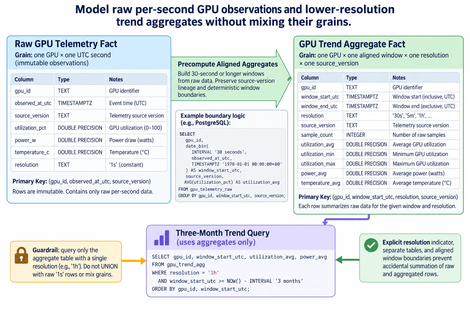
Create separate compatible structures for immutable per-second telemetry and precomputed thirty-second or longer-window summaries. Specify keys, measures, aggregation window boundaries, source-version lineage, and a resolution indicator so a three-month trend query cannot accidentally sum raw and aggregated rows together.

Short Interview Answer (30-60 seconds)

I would keep raw per-second telemetry and trend aggregates in separate fact tables. Raw rows stay immutable. Aggregate rows have explicit aligned window boundaries, source-version lineage, and resolution. Long-range trend queries read only the aggregate table and filter to exactly one resolution.

Detailed Explanation

See the Code while reading this explanation.

The problem is that the same GPU activity can appear at different levels of detail. One dataset records every second, while another stores summaries for longer periods. If both kinds of rows are treated as one dataset, a report can count the same underlying activity more than once. The safe design is to store them separately, clearly record how much time each row represents, keep the original observations unchanged, preserve where every summary came from, and make long-term reports choose exactly one summary level before calculating trends.

Useful Questions to Ask the Interviewer
  1. Which aggregate resolutions must be supported beyond 30 seconds, such as 5 minutes or 1 hour?
  2. Should all aggregation windows use UTC-aligned boundaries?
  3. Can the same observation be reprocessed under a new source version?
  4. Which measures require average, minimum, maximum, or other summary functions?
Model raw per-second GPU observations and lower-resolution trend aggregates without mixing their grains. diagram
How to Explain It in an Interview

Assume a current PostgreSQL version that supports date_bin, because the approved diagram uses PostgreSQL syntax for its boundary example.

The raw structure is gpu_telemetry_raw. Its declared time grain is one GPU observation per UTC second, and source_version participates in the primary key so different lineage versions do not overwrite each other. The primary key is (gpu_id, observed_at_utc, source_version). The table stores gpu_id, observed_at_utc, source_version, utilization_pct, power_w, temperature_c, and a resolution value fixed to '1s'. Rows are immutable and contain only raw per-second observations.

The aggregate structure is gpu_trend_agg. Its grain is one GPU times one aligned aggregation window times one resolution times one source version. Its primary key is (gpu_id, window_start_utc, resolution, source_version). window_start_utc is inclusive and window_end_utc is exclusive. The table stores resolution, source_version, sample_count, utilization_avg, utilization_min, utilization_max, power_avg, and temperature_avg.

The transformation reads raw telemetry and precomputes non-overlapping aligned windows of 30 seconds or longer. In the diagram, PostgreSQL date_bin(INTERVAL '30 seconds', observed_at_utc, TIMESTAMPTZ '1970-01-01 00:00:00+00') creates a deterministic window_start_utc. A 30-second aggregate would have an exclusive window_end_utc 30 seconds after that start. Longer resolutions follow the same explicit boundary rule.

Source-version lineage is carried into the aggregate grain. This means summaries created from different source interpretations or processing versions are not silently merged together. The lineage can be selected deliberately when reproducing or rebuilding a trend.

The resolution column is the key semantic guardrail. Raw rows use '1s', while aggregate rows may use values such as '30s', '5m', or '1h'. A three-month trend query reads only gpu_trend_agg and filters to one resolution, for example resolution = '1h'. It must not UNION raw '1s' rows with aggregate rows or combine several aggregate resolutions in one additive calculation.

This design gives two clear access paths. Detailed investigation and rebuilding use immutable raw telemetry. Long-range analysis uses precomputed aggregates. The tradeoff is extra storage and aggregation work, but the model reduces long-range scan volume and, more importantly, makes accidental mixed-grain calculations much harder.

The approved diagram does not define nullability, indexes, table partitioning, duplicate handling outside the declared primary keys, or a physical query plan. Those details should be chosen from real ingestion and workload requirements instead of being invented.

Technical Approach
  1. Declare the raw observation grain and primary key.
  2. Store per-second telemetry immutably with resolution = '1s' and source-version lineage.
  3. Precompute aligned, non-overlapping windows of 30 seconds or longer from raw rows.
  4. Store one aggregate row per GPU, window, resolution, and source version.
  5. Record inclusive window_start_utc, exclusive window_end_utc, sample_count, aggregate measures, lineage, and resolution.
  6. Make long-range consumers query only gpu_trend_agg.
  7. Require each trend query to filter to exactly one resolution, such as '1h'.
  8. Never combine raw and aggregate rows in the same additive metric calculation.
Practical Insights

Raw storage grows quickly because every GPU can produce one observation each second. Aggregate storage grows much more slowly because many raw observations become one summary row. Building summaries requires reading the raw rows for each window and calculating measures once. A three-month trend then reads far fewer aggregate rows than raw seconds. The operational cost is maintaining both raw and aggregate data and rebuilding summaries when lineage changes, but the benefit is safer long-range queries and lower read volume.

Code
-- Build a 30-second aggregate grain from immutable raw telemetry.
-- The fixed UTC origin gives deterministic aligned 30-second window starts.
-- Keep gpu_id and source_version in the grouping grain so lineage is not mixed.
SELECT
  gpu_id,
  date_bin (
    INTERVAL '30 seconds',
    observed_at_utc,
    TIMESTAMPTZ '1970-01-01 00:00:00+00'
  ) AS window_start_utc,
  source_version,
  AVG(utilization_pct) AS utilization_avg
FROM
  gpu_telemetry_raw
GROUP BY
  gpu_id,
  window_start_utc,
  source_version;


-- Read only the aggregate fact for the long-range trend.
-- Select exactly one resolution so different grains cannot be combined.
-- ORDER BY makes the returned GPU trend deterministic for presentation.
SELECT
  gpu_id,
  window_start_utc,
  utilization_avg,
  power_avg
FROM
  gpu_trend_agg
WHERE
  resolution = '1h'
  AND window_start_utc >= NOW () - INTERVAL '3 months'
ORDER BY
  gpu_id,
  window_start_utc;
Why Interviewers Ask This

This tests whether the candidate understands grain as a core data-modeling contract. The interviewer wants to see whether the candidate can keep raw observations and summaries separate, define stable keys and time boundaries, preserve lineage, choose appropriate aggregate measures, and design consumer queries that cannot silently double-count data by mixing resolutions.

Common interview mistakes

The biggest mistake is storing raw and aggregate rows together without a strict grain boundary. Other mistakes are omitting resolution from the aggregate key, losing source_version lineage, using ambiguous or overlapping window boundaries, grouping different source versions together, failing to state inclusive-start and exclusive-end semantics, and querying multiple resolutions together. A particularly dangerous error is to UNION raw '1s' rows with '30s', '5m', or '1h' rows and then aggregate them, because the same underlying observations can be counted more than once.

Interview tip

Lead with the grain. State the raw grain and aggregate grain, then give both primary keys. Next explain aligned [start, end) windows, source-version lineage, and the one-resolution query rule. That shows immediately how the model prevents mixed-grain double counting.

Interviewer may ask next
Why include resolution in the aggregate primary key if window_start_utc is already present?

The same GPU and window start can have several valid summaries, such as '30s', '5m', and '1h'. window_start_utc alone therefore does not identify the aggregation grain. Including resolution in (gpu_id, window_start_utc, resolution, source_version) allows those summaries to coexist without key collisions and makes the grain explicit.

What should happen if telemetry is reprocessed with a new source version?

Keep the original raw observations immutable and retain source_version in both raw and aggregate keys. Build summaries under the new source version instead of overwriting the old lineage. Trend consumers should select the intended lineage consistently so summaries produced from different source versions are not silently combined.

3. Model schema evolution when GPU architectures, drivers, or AI frameworks change telemetry metrics.Data ModelingMediumNvidia

Question Details

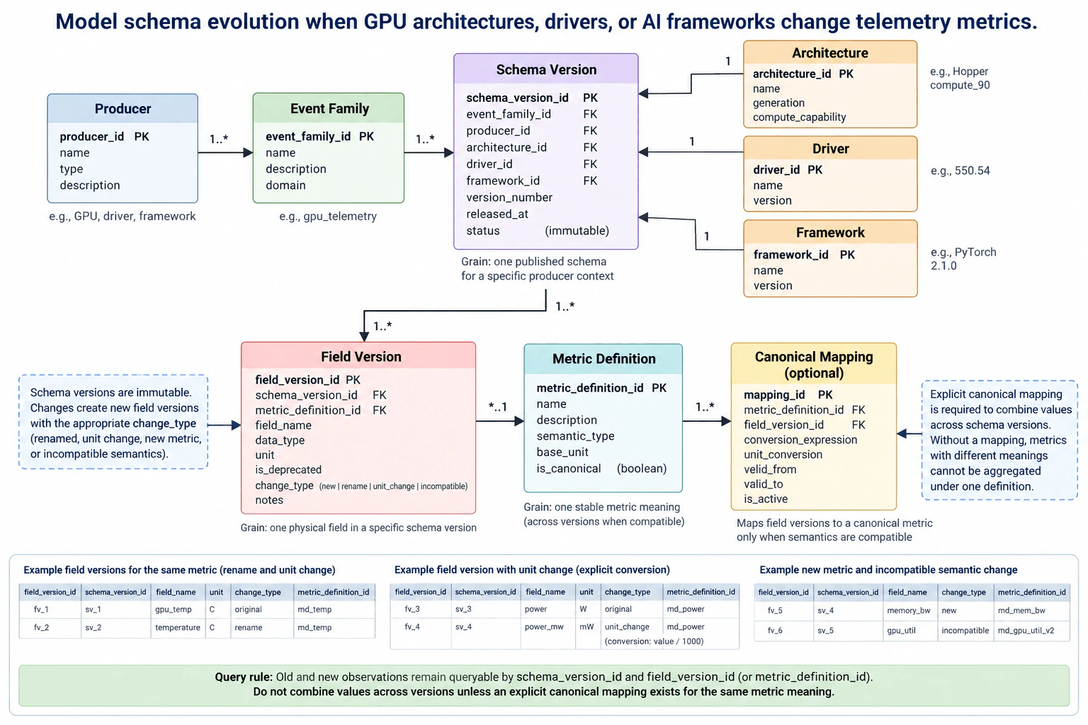
Define event-family, producer, architecture, driver, framework, metric-definition, schema-version, and field-version entities. Show how renamed fields, changed units, new metrics, and incompatible semantics are recorded so old and new observations remain queryable but cannot be combined under one meaning without an explicit canonical mapping.

Short Interview Answer (30-60 seconds)

Version schemas and fields instead of overwriting them. Keep stable meaning in metric-definition, record renames, unit changes, new metrics, and incompatible changes in field-version, and require an explicit canonical mapping before observations from different versions are combined.

Detailed Explanation

The main decision is how to keep measurements useful when hardware or software changes what is reported. I would never replace the old description with the new one. Every published form gets its own identity, and every reported value keeps the identity of the exact field that produced it. A name change, measurement-unit change, newly added value, or meaning change becomes another recorded version. Past data stays readable. New data also stays readable. The key safety rule is that values with different meanings are never mixed unless an explicit mapping says they represent the same thing.

Useful Questions to Ask the Interviewer
  1. Can a producer publish several schema versions for the same event family at the same time?
  2. Should compatible unit changes be converted to one canonical unit during reads, or should consumers choose the conversion?
  3. Who owns approval of canonical mappings when two field versions are considered semantically compatible?
  4. Do architecture, driver, and framework changes always create a new schema version, or only when the emitted fields change?
Model schema evolution when GPU architectures, drivers, or AI frameworks change telemetry metrics. diagram
How to Explain It in an Interview

Start with immutable schema history. A schema-version represents one published schema for a specific producer context. It has schema_version_id as its primary key and references event_family_id, producer_id, architecture_id, driver_id, and framework_id. It also records version_number, released_at, and status. Once published, that version is not edited. A schema change creates another schema-version record.

The event-family entity groups related telemetry events. Producer identifies the component that emits the telemetry. Architecture, driver, and framework describe the environment associated with the schema version. Keeping these as separate entities lets a query distinguish observations produced under different GPU generations, driver versions, or AI framework versions without destroying history.

Next, separate the physical field from the metric meaning. A field-version is one physical field in one specific schema version. Its fields include field_version_id, schema_version_id, metric_definition_id, field_name, data_type, unit, is_deprecated, change_type, and notes. The change_type records whether that version is new, renamed, changed in unit, or incompatible in meaning.

A metric-definition represents one stable metric meaning. It contains metric_definition_id, name, description, semantic_type, base_unit, and is_canonical. The direct metric_definition_id on field-version records the field's declared meaning. A rename does not automatically create a new meaning. For example, the diagram shows gpu_temp renamed to temperature while both field versions remain associated with md_temp.

A compatible unit change also creates a new field-version without rewriting history. The diagram shows power in W and power_mw in mW as different field versions associated with md_power. The conversion is explicit: the mW value is divided by 1000 to reach W. The meaning is stable, but the physical representation changed.

A genuinely new metric receives its own field version and metric definition. The diagram shows memory_bw as a new field associated with md_mem_bw. An incompatible semantic change must also be separated. The example shows gpu_util marked incompatible and associated with md_gpu_util_v2 instead of pretending it has the old meaning.

Canonical Mapping is the explicit authorization for combining field versions under one canonical interpretation. It contains mapping_id, metric_definition_id, field_version_id, conversion_expression, unit_conversion, valid_from, valid_to, and is_active. This mapping can confirm semantic compatibility and record the conversion needed to normalize units. Without that mapping, similar names or related metric definitions are not enough to justify aggregation.

Historical observations therefore remain queryable through schema_version_id and field_version_id, or through their associated metric_definition_id. Consumers can inspect old and new values independently. They may combine values across schema versions only when an explicit canonical mapping exists for the same metric meaning. This prevents a renamed field, changed unit, or incompatible semantic change from silently corrupting historical analysis.

The tradeoff is additional metadata and governance. Every evolution creates more immutable schema and field records, and canonical mappings require review. In return, historical interpretation remains reproducible, producer context is retained, and consumers cannot accidentally merge measurements whose names look similar but whose meanings differ.

Technical Approach
  1. Identify the event-family and producer that own the telemetry event.
  2. Create an immutable schema-version for the published producer, architecture, driver, and framework context.
  3. Create one field-version for each physical field in that schema version.
  4. Link each field-version to the metric-definition representing its declared semantic meaning.
  5. For a rename, create a new field-version and keep the same metric-definition when meaning and unit are unchanged.
  6. For a compatible unit change, create a new field-version and record the approved conversion in canonical mapping.
  7. For a new metric, create a new field-version and a corresponding metric-definition.
  8. For incompatible semantics, create a new field-version with a different metric-definition instead of reusing the old meaning.
  9. Keep observations queryable using their schema-version and field-version identities.
  10. Combine versions only when an explicit canonical mapping confirms compatible meaning and any required unit conversion.
Practical Insights

The runtime cost is mainly a small amount of metadata lookup before telemetry values are interpreted or combined. Historical observations still point to specific schema and field versions, so old data remains directly traceable. Storage grows because old schema-version and field-version records are retained instead of overwritten, but this metadata is usually much smaller than the telemetry itself. The larger cost is operational: producers must publish versions correctly, mappings require governance, and consumers must use the mapping instead of grouping values only because field names look similar.

Why Interviewers Ask This

This tests whether the candidate can preserve historical telemetry while allowing producers, GPU architectures, drivers, and AI frameworks to evolve. A strong answer separates physical field versions from stable metric meaning, keeps schema history immutable, handles renames and unit changes safely, and prevents incompatible measurements from being silently combined.

Common interview mistakes

Common mistakes are overwriting an old schema instead of creating a new immutable version; treating field_name as the metric identity; creating a new semantic meaning for a simple rename; assuming identical names mean identical semantics; converting units implicitly without an approved mapping; reusing the old metric definition after an incompatible semantic change; deleting deprecated field versions; and aggregating observations across schema versions merely because their fields look similar. Another mistake is losing the architecture, driver, or framework context required to interpret historical schemas.

Interview tip

Draw a clear boundary between physical representation and semantic meaning. Say that schema-version preserves published context, field-version preserves physical field history, metric-definition owns stable meaning, and canonical mapping is the explicit gate for safe cross-version aggregation. Then walk through rename, unit-change, new-metric, and incompatible-semantics cases.

Interviewer may ask next
How would you handle a field that changes from watts to milliwatts but keeps exactly the same meaning?

Create a new field-version under the new schema-version and keep it associated with the same metric-definition. Record change_type as unit_change and retain the original W field version unchanged. Add an explicit canonical mapping for the mW field version with the required conversion to the canonical unit. In the diagram's example, converting mW to W is value divided by 1000. Queries may read both versions separately or combine them only through that approved mapping.

What should happen if a telemetry field keeps a similar name but its semantics become incompatible?

Treat it as a semantic break. Create a new field-version with change_type incompatible and associate it with a different metric-definition representing the new meaning, as the diagram does with md_gpu_util_v2. Keep the previous field version and meaning unchanged so historical observations remain reproducible. Do not aggregate the old and new values under one meaning unless a later explicit canonical mapping can defensibly establish compatibility; otherwise they remain separate.

4. Design the analytical schema for multi-region autonomous-robotics safety logs.Data ModelingHardNvidia

Question Details

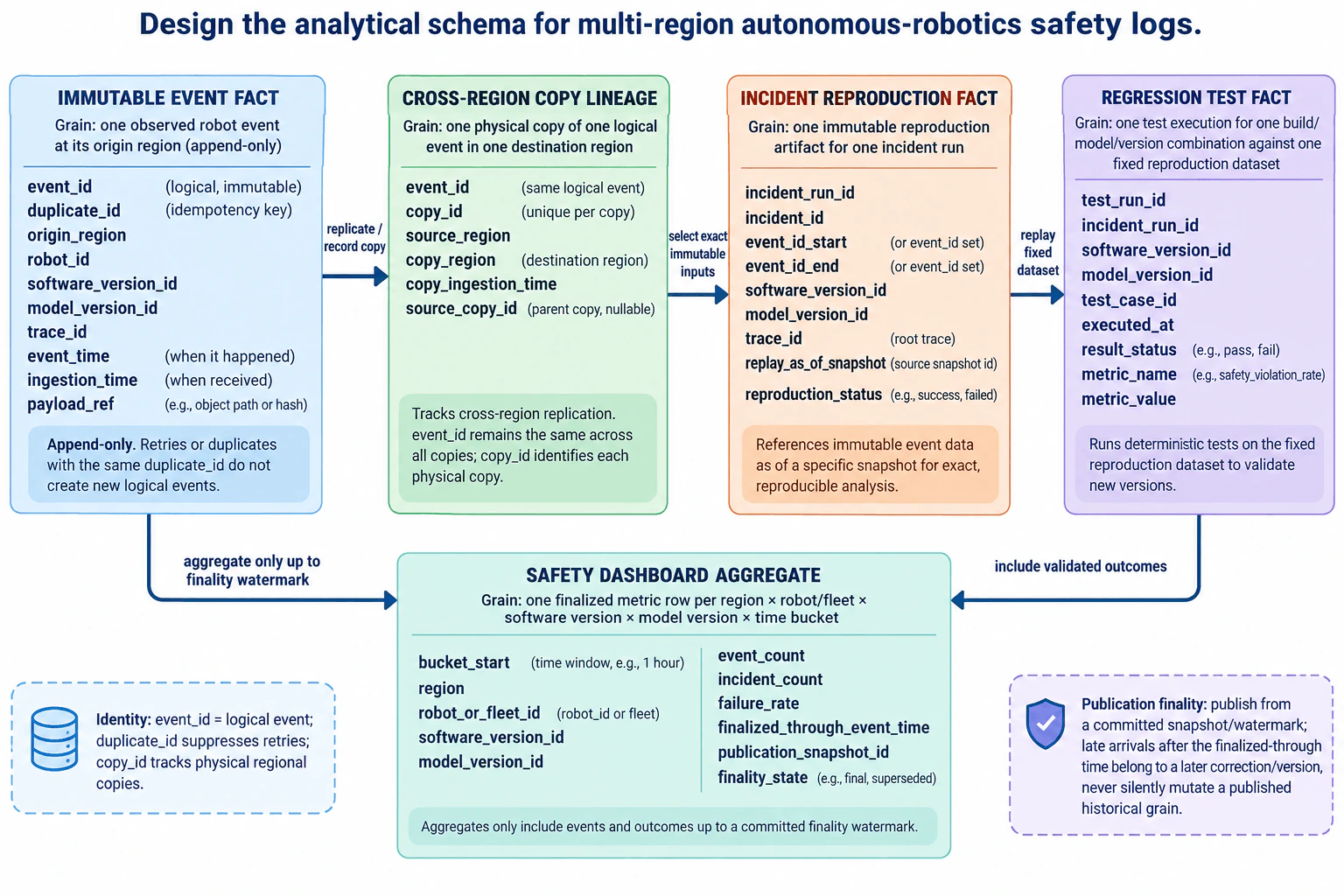
Declare immutable event, incident-reproduction, regression-test, and safety-dashboard aggregate grains for fleet logs that can burst to millions of events per second. Include region, vehicle or robot, software and model versions, trace identity, event and ingestion times, duplicate identity, cross-region copy lineage, and publication finality.

Short Interview Answer (30-60 seconds)

I would keep immutable robot events as the source of truth, track each regional copy separately, freeze exact event inputs for incident reproduction, store one row per regression-test execution, and publish aggregates only through a committed finality watermark so late data creates a later correction instead of rewriting history.

Detailed Explanation

The system needs to keep a trustworthy history of what every robot reported, even when the same record reaches several regions or is sent more than once. It also needs to recreate a safety incident later, test new software and models against the same evidence, and publish stable dashboard numbers. The key decision is to keep original records unchanged, identify copied records separately, save the exact evidence used for each recreation, record each test run, and publish summaries only after the system has declared a time range complete.

Useful Questions to Ask the Interviewer
  1. Is event_id globally unique for the same logical robot event across every region?
  2. What exactly defines duplicate_id: a producer-generated idempotency key, a deterministic identity, or another contract?
  3. Can copies be replicated from other copies, requiring source_copy_id to preserve the complete parent-copy lineage?
  4. Does an incident reproduction always use a contiguous event range, or can it reference an explicit event-id set?
  5. What business rule advances the committed publication finality watermark?
  6. When data arrives after finality, should the system publish a superseding aggregate version rather than mutate the previous publication?
  7. Does robot_or_fleet_id represent individual-robot dashboard rows, fleet-level rows, or both?
Design the analytical schema for multi-region autonomous-robotics safety logs. diagram
How to Explain It in an Interview

Start with the IMMUTABLE EVENT FACT. Its grain is one observed robot event at its origin region. It is append-only. event_id is the immutable logical event identity. duplicate_id is the idempotency identity used to recognize retries or duplicate delivery so they do not create new logical events. The row also carries origin_region, robot_id, software_version_id, model_version_id, trace_id, event_time, ingestion_time, and payload_ref. event_time means when the event happened on the robot; ingestion_time means when the platform received it. Keeping both matters because network delay and late arrival make those times different.

Keep CROSS-REGION COPY LINEAGE separate from the logical event fact. Its grain is one physical copy of one logical event in one destination region. It contains event_id, copy_id, source_region, copy_region, copy_ingestion_time, and nullable source_copy_id. event_id remains the same across all copies of the logical event. copy_id uniquely identifies a physical regional copy. source_copy_id records the parent copy when replication continues from a previously copied event. This prevents replication from multiplying the logical event grain and corrupting analytical counts.

For the INCIDENT REPRODUCTION FACT, use one immutable reproduction artifact for one incident run. Give it incident_run_id and incident_id and bind it to the exact immutable source inputs. The diagram represents those inputs with event_id_start and event_id_end, or an explicit event-id set when the incident is not naturally contiguous. Also record software_version_id, model_version_id, the root trace_id, replay_as_of_snapshot, and reproduction_status. replay_as_of_snapshot identifies the source snapshot used for exact reproducible analysis. A later attempt should create another immutable reproduction run rather than silently overwrite the prior artifact.

The REGRESSION TEST FACT has another grain: one test execution for one build or software/model-version combination against one fixed reproduction dataset. Store test_run_id, incident_run_id, software_version_id, model_version_id, test_case_id, executed_at, result_status, metric_name, and metric_value. incident_run_id ties every result back to the exact fixed reproduction dataset. This makes test outcomes attributable even while the live fleet event stream continues to grow.

The SAFETY DASHBOARD AGGREGATE has the grain shown in the diagram: one finalized metric row per region × robot or fleet × software version × model version × time bucket. Its dimensional fields are bucket_start, region, robot_or_fleet_id, software_version_id, and model_version_id. Its measures and publication metadata include event_count, incident_count, failure_rate, finalized_through_event_time, publication_snapshot_id, and finality_state.

The publication rule is central. Aggregate only events and validated outcomes up to a committed finality watermark. finalized_through_event_time states how far event time is considered complete for that publication. publication_snapshot_id identifies the published snapshot. finality_state can represent states such as final or superseded. If a late event arrives after the finalized-through boundary, do not silently mutate the previously published historical grain. Publish a later correction or superseding version instead so previous dashboard results remain reproducible and auditable.

The end-to-end flow is therefore: append one immutable logical event, record each cross-region physical copy in lineage, select exact immutable inputs for an incident reproduction, replay the fixed snapshot, execute regression tests against that fixed reproduction dataset, and aggregate finalized events plus validated outcomes into dashboard rows.

For a fleet that can burst to millions of events per second, keep the high-volume immutable event fact as the atomic analytical source of truth and keep physical copy lineage separate. Dashboard users should normally read precomputed aggregate rows rather than repeatedly scanning raw events. The exact partitioning, clustering, indexing, storage format, and warehouse-specific implementation depend on the database engine, which the question does not specify.

The main tradeoff is extra storage and pipeline complexity versus reproducibility. Immutable events, copy lineage, frozen reproduction artifacts, independent regression runs, and versioned aggregate publications consume more storage. In return, retries are explicit, regional copies cannot inflate logical counts, incident investigations remain reproducible, regression results remain tied to exact data and versions, and published dashboard history remains auditable.

Technical Approach
  1. Declare the immutable event grain as one logical observed robot event at its origin region and make it append-only.
  2. Use event_id for logical identity and duplicate_id for retry or duplicate identity.
  3. Store one cross-region lineage row per physical regional copy, using copy_id as the physical-copy identity and source_copy_id for parent-copy lineage.
  4. Create one immutable incident-reproduction artifact per run and bind it to an exact event range or explicit event-id set plus replay_as_of_snapshot.
  5. Store one regression-test fact per test execution against that fixed reproduction dataset and version combination.
  6. Aggregate at region × robot/fleet × software version × model version × time-bucket grain.
  7. Publish aggregates only through a committed finality watermark using finalized_through_event_time, publication_snapshot_id, and finality_state.
  8. Handle post-finality late arrivals with a later correction or superseding publication rather than mutating published historical rows.
Practical Insights

Raw storage grows with the number of logical events, physical regional copies, incident-reproduction runs, regression-test executions, and published aggregate versions. The immutable event fact carries the largest write volume because the fleet can burst to millions of events per second. Copy lineage adds storage but prevents replication from being mistaken for new events. Reproduction and regression facts add smaller amounts of data while making investigations repeatable. Precomputed dashboard aggregates require extra pipeline work but avoid repeatedly scanning raw telemetry. Publication finality also adds operational state because the system must advance a committed watermark and issue later versions when late data changes an already finalized period.

Why Interviewers Ask This

This question tests whether the candidate can define precise analytical grains for a fleet that can burst to millions of events per second while keeping identity, duplicate handling, multi-region replication, incident reproduction, version history, regression testing, and published metrics trustworthy. A strong answer separates logical events from physical copies, freezes reproduction inputs, records tests at execution grain, and gives dashboard aggregates an explicit publication-finality contract.

Common interview mistakes

Common mistakes are treating every regional copy as a new logical event and inflating counts; using only ingestion_time and losing when the event actually happened; using only event_time and losing arrival behavior; confusing event_id, duplicate_id, and copy_id; putting physical replication fields directly into the logical event grain; overwriting an incident-reproduction artifact when inputs change; running regression tests against a moving live event set instead of the fixed reproduction dataset; omitting software_version_id or model_version_id from reproducibility records; publishing aggregates without an explicit finality boundary; and silently rewriting previously published dashboard history after late data arrives.

Interview tip

Lead with the five grains visible in the diagram: one immutable logical event, one physical regional copy, one immutable incident-reproduction artifact, one regression-test execution, and one finalized dashboard metric row. Then explain identity and finality: event_id stays stable, duplicate_id handles retry identity, copy_id distinguishes physical copies, and late data creates a later publication version instead of silently rewriting history.

Interviewer may ask next
How would you prevent retries and cross-region replication from inflating safety metrics?

Count the immutable logical event grain, not physical copies. event_id identifies the same logical event across regions. duplicate_id is the idempotency identity used to recognize retries or duplicate delivery. Each physical regional replica receives its own copy_id in the cross-region lineage table while retaining the same event_id. Dashboard aggregation therefore operates on logical events through the committed finality boundary, so additional regional copies do not increase event_count.

What should happen when an event arrives after a dashboard period has already been finalized?

Do not silently mutate the published historical row. The aggregate records finalized_through_event_time, publication_snapshot_id, and finality_state. A late event that belongs to an already finalized period should be reflected in a later correction or superseding publication version. The previous publication stays reproducible, while the newer snapshot contains the corrected metric state. This requires additional storage and publication logic, but it preserves auditability and prevents one publication identifier from producing different historical results over time.

5. Process real-time telemetry when network connectivity is intermittent.Data PipelinesEasyNvidia

Question Details

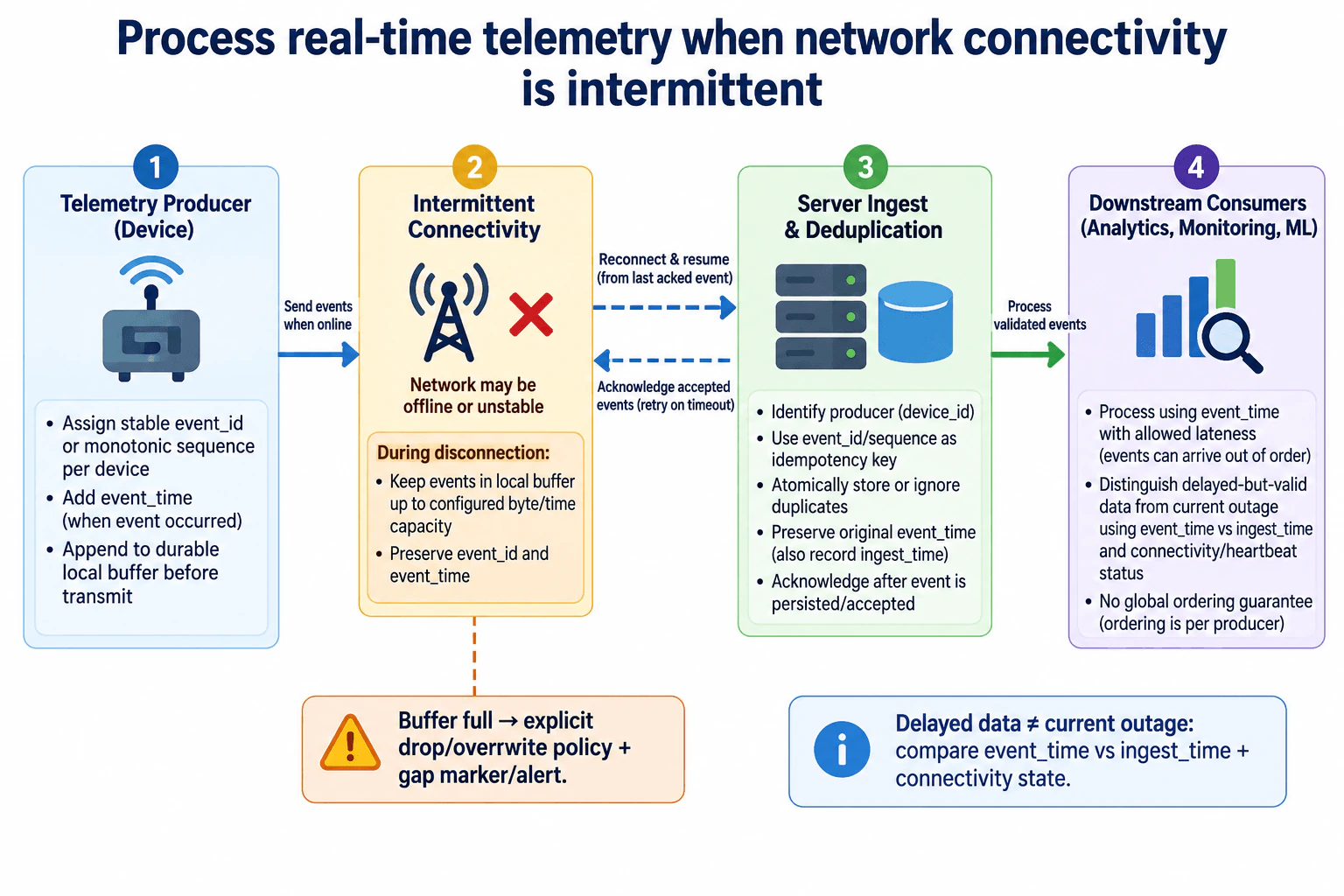
Define producer-side buffering, sequence or event identifiers, reconnect handshakes, retry and acknowledgement rules, retention limits, event-time ordering, and server-side deduplication. Include the behavior when the offline interval exceeds local capacity and how downstream consumers distinguish delayed but valid data from a current outage.

Short Interview Answer (30-60 seconds)

I would buffer telemetry durably on the device, give every event a stable ID or per-device sequence and its original event time, and retry unacknowledged events after reconnecting. The server deduplicates before accepting them and then acknowledges them. Downstream consumers process by event time with allowed lateness. The key trade-off is finite local capacity: if an outage lasts too long, the system needs an explicit drop or overwrite policy plus a visible gap marker or alert.

Detailed Explanation

The goal is to keep useful measurements when a device temporarily cannot reach the server. The device should continue saving what it observes instead of throwing it away immediately. When the connection returns, it should send the missing information again without creating extra copies. The receiving side must know what is new, what was already accepted, and when each measurement originally happened. Local storage is limited, so a very long outage can still cause loss. That loss must be made visible. Consumers must also tell old information arriving late from a device that is currently unreachable.

Useful Questions to Ask the Interviewer
  1. How much local byte or time capacity can each producer reserve for offline telemetry?
  2. If that capacity is exceeded, should the producer drop oldest events, overwrite according to a defined policy, or stop accepting new telemetry?
  3. Is ordering required only per producer, or is any wider ordering guarantee required?
  4. How late may delayed events arrive before downstream processing stops accepting them into event-time results?
  5. What connectivity or heartbeat signal is available to identify a current outage?
Process real-time telemetry when network connectivity is intermittent. diagram
How to Explain It in an Interview
1. Identify and buffer each event at the producer

I would start at the Telemetry Producer. Each event gets a stable event_id or a monotonic sequence scoped to that device, plus event_time, which records when the event occurred. Before transmission, the producer appends the event to a durable local buffer. If a retry happens later, the producer reuses the same identifier and original event_time. This gives the server a stable way to recognize the same logical event more than once.

2. Keep buffering while connectivity is unavailable

When the network is available, buffered events move toward Server Ingest & Deduplication. When connectivity becomes offline or unstable, the device continues retaining events locally up to a configured byte or time capacity. That capacity is intentionally bounded. If the offline period exceeds it, the producer follows an explicit drop or overwrite policy and creates a gap marker or alert. This prevents silent loss and avoids pretending local storage can grow forever.

3. Resume from the last acknowledgement

After reconnecting, the producer resumes from the last acknowledged event and retries events that may not have been acknowledged. The acknowledgement travels from Server Ingest back to the producer. It is sent only after an event has been persisted or accepted at the server boundary. If the acknowledgement itself is lost, the producer may send that event again. The retry is safe because its event identity does not change.

4. Deduplicate at Server Ingest

Server Ingest & Deduplication identifies the producer by device_id and uses event_id or sequence with that producer identity as the idempotency key. Idempotency means repeating the same logical operation does not create another logical result. The server atomically stores a new event or ignores an already accepted duplicate. It preserves the original event_time and also records ingest_time, which is when the server received the event. This separates repeated transport attempts from duplicate business data.

5. Process using event time and per-producer ordering

Validated events move to Downstream Consumers. They process using event_time with an allowed-lateness rule because reconnecting devices can send older buffered events after newer events have already arrived elsewhere. The design does not claim global ordering. A monotonic sequence provides ordering only for that producer. Allowed lateness defines how long downstream processing remains willing to incorporate delayed but valid events.

6. Separate delayed data from a current outage

Consumers compare event_time with ingest_time to see whether an arriving event is old, and they use connectivity or heartbeat state to determine whether the producer is currently reachable. An old event that arrives after reconnection is delayed but valid. A missing current connectivity or heartbeat signal indicates a current outage condition. Keeping those signals separate prevents late telemetry from being mistaken for current device health.

7. State the recovery limit clearly

This design handles ordinary disconnects, retries, duplicate transmissions, and lost acknowledgements while the required events remain in the local buffer. It does not promise zero loss if the outage lasts beyond local capacity. Once the configured capacity is exhausted, the explicit drop or overwrite policy applies, and the gap marker or alert makes that missing interval visible.

Technical Approach
  1. Assign each event a stable event_id or monotonic per-device sequence and its original event_time.
  2. Append the event to a durable bounded local buffer before transmission.
  3. Send buffered events while connected.
  4. During an outage, retain them locally until the configured byte or time capacity is reached.
  5. On reconnect, resume from the last acknowledged event and retry unacknowledged records.
  6. At Server Ingest & Deduplication, identify the producer and use device_id plus event_id or sequence as the idempotency key.
  7. Atomically persist a new event or ignore a duplicate, then acknowledge the accepted event.
  8. Preserve event_time and record ingest_time.
  9. Downstream, process by event_time with allowed lateness and per-producer ordering only.
  10. If local capacity is exceeded, apply the explicit drop or overwrite policy and emit a gap marker or alert.
  11. Distinguish delayed data from a current outage using event_time versus ingest_time together with connectivity or heartbeat state.
Practical Insights

The benefit is that temporary network failures do not immediately lose telemetry, and retries are safe because the server deduplicates using a stable event identity. The downside is extra storage and state. A larger local buffer tolerates longer outages but consumes more device storage. Longer allowed lateness lets more delayed events affect event-time results, but those results may take longer to settle. Keeping deduplication information available for longer makes very late retries easier to recognize, but it also needs more server state. We accept these costs because intermittent connectivity is expected. The important limit is finite local capacity: once an outage exceeds that capacity, the configured drop or overwrite policy can cause explicit data loss.

Why Interviewers Ask This

This question tests whether a candidate can preserve correctness when a real-time stream temporarily stops being real time. The interviewer is looking for judgment around durable buffering, identifiers, retries, acknowledgements, duplicate handling, ordering, late events, bounded storage, and recovery. It also checks whether the candidate understands the difference between when data happened and when it arrived, and can explain the trade-offs without claiming global ordering, unlimited buffering, or guaranteed zero loss.

Common interview mistakes

Common mistakes are transmitting before making the event durable locally, creating a new event_id on every retry, acknowledging before Server Ingest has accepted the event, and assuming retries cannot create duplicates. Another mistake is treating ingest_time as event_time, which can make delayed telemetry appear current. Candidates may also claim global ordering even though the shown sequence is only per producer. A major operational mistake is forgetting that the local buffer is finite. If an outage exceeds its configured capacity, the design needs an explicit drop or overwrite policy plus a gap marker or alert. Finally, an old event does not prove the producer is currently offline; current connectivity or heartbeat state is a separate signal.

Interview tip

Explain the design as one recovery loop: identify and buffer locally, reconnect from the last acknowledgement, retry safely, deduplicate at ingest, and process with the original event time. Explicitly state that ordering is per producer and that finite local capacity prevents a guaranteed zero-loss claim. That demonstrates both correctness and practical operational judgment.

Interviewer may ask next
What changes if the device stays offline longer than the local buffer can retain telemetry?

The architecture stays the same, but the retention boundary becomes the main decision. The Telemetry Producer still assigns stable event IDs or per-device sequences, records event_time, and writes events to the durable local buffer. The changed requirement is that the producer reaches its configured byte or time capacity before connectivity returns. At that point it applies the explicit policy shown in the design: drop or overwrite according to the chosen rule, then create a gap marker or alert so the missing interval is visible. I would not claim those discarded events can be recovered later. After reconnecting, the producer resumes with the events that remain, starting from the last acknowledged position and using the same retry rules. Server Ingest & Deduplication still prevents repeated accepted results and acknowledges accepted events. Downstream consumers distinguish the gap from delayed valid telemetry. No new security mechanism or security boundary is introduced by this change. The downside is unavoidable loss after bounded local capacity is exhausted, so retention size and the drop policy must match the value of the telemetry.

How do downstream consumers tell a late replayed event from evidence that the producer is currently offline?

I would keep timing and current connectivity as separate signals. Each event keeps its original event_time from the Telemetry Producer, while Server Ingest records ingest_time when it accepts the event. If a producer reconnects and sends an older buffered event, the difference between event_time and ingest_time shows that the event arrived late. Downstream Consumers can still process it under the configured allowed-lateness rule. To decide whether the producer is currently offline, they use the separate connectivity or heartbeat state shown in the design. An old event alone does not mean the device is offline now, and a current heartbeat failure does not make previously buffered data invalid. Server-side deduplication remains unchanged, so repeated transmissions with the same device_id and event_id or sequence do not create duplicate accepted events. No new security mechanism or security boundary is required for this distinction. The main downside is that consumers must reason about two timestamps and a separate liveness signal, but that separation prevents stale telemetry from being mistaken for current system health.

6. Design real-time ingestion for high-volume events from many devices.Data PipelinesEasyNvidia

Question Details

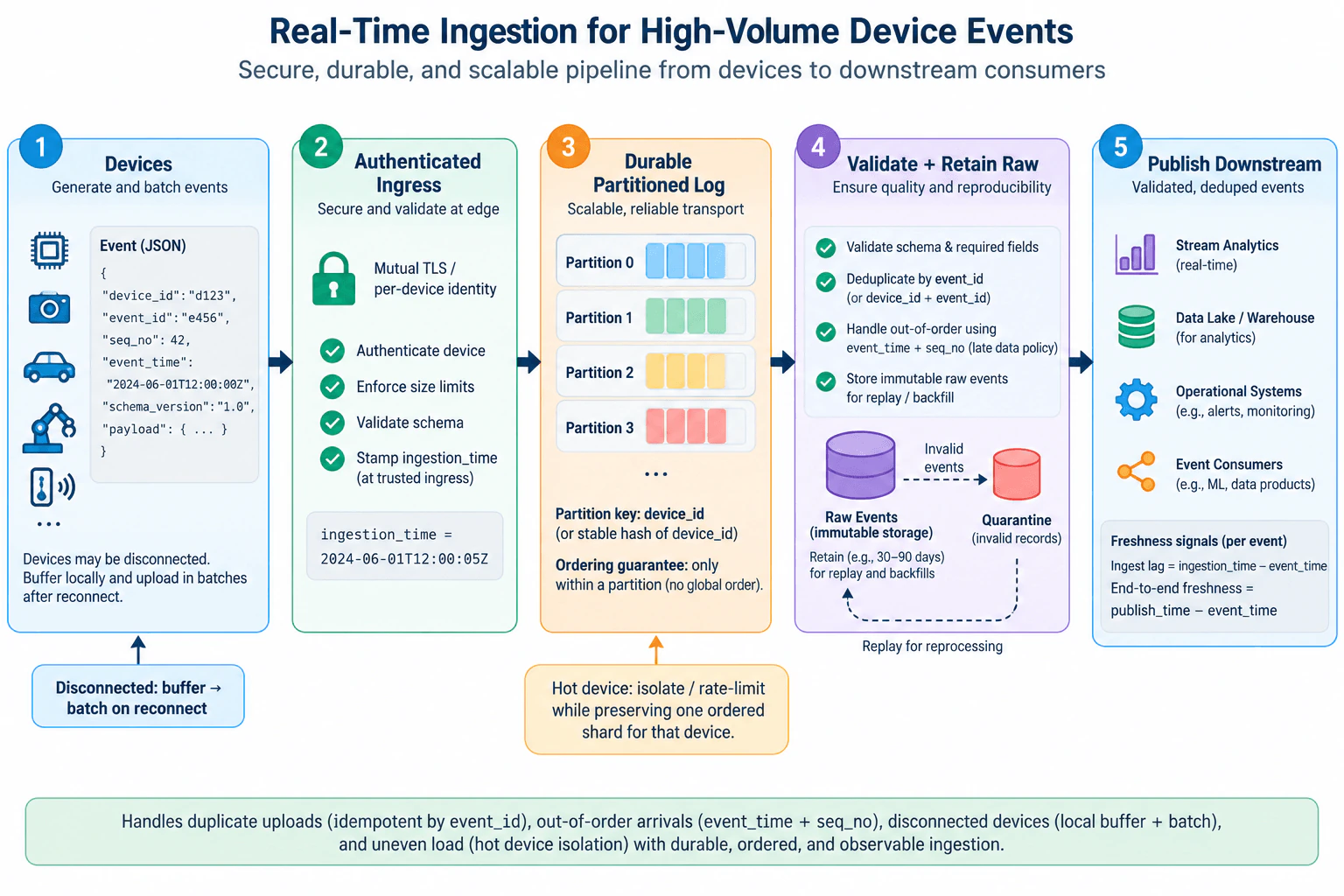
Specify the device event contract, authentication boundary, batching, durable transport, partition key, event and ingestion timestamps, validation, raw retention, and downstream publication. Cover disconnected devices, duplicate uploads, out-of-order arrivals, one unusually hot device, and the end-to-end freshness signal.

Short Interview Answer (30-60 seconds)

I would have devices buffer and batch events, authenticate each device at ingress, stamp ingestion_time, and append accepted events to a durable log partitioned by device_id. Then I would validate and deduplicate events, retain immutable raw data for replay, quarantine invalid records, and publish validated events downstream. The main trade-off is that preserving per-device ordering makes a very hot device harder to distribute, so it may need isolation or rate limiting.

Detailed Explanation

The goal is to move a large number of device events into downstream systems quickly without losing the ability to understand, validate, or replay them. Each event needs a clear identity, its original device time, and enough information to detect repeated uploads. Devices may lose connectivity, so they should buffer events and send them later in batches. The pipeline should keep one device's events in a useful order, isolate bad records, keep an original copy for recovery, and show how long each event takes to reach downstream consumers.

Useful Questions to Ask the Interviewer
  1. How long can a device stay disconnected before its local buffer becomes a concern?
  2. How long should immutable raw events be retained for replay or backfill?
  3. What end-to-end freshness is expected by downstream consumers?
  4. What behavior is preferred when one device produces far more traffic than normal?
Design real-time ingestion for high-volume events from many devices. diagram
How to Explain It in an Interview
1. Define the device event contract

I would start with the event contract shown in the diagram. Each JSON event contains device_id, event_id, seq_no, event_time, schema_version, and payload. device_id identifies the producer. event_id is the idempotency key used to recognize duplicate uploads. seq_no helps reason about the order generated by one device. event_time records when the device says the event occurred. schema_version identifies the event contract version.

Devices generate events continuously but upload them in batches. When disconnected, a device buffers locally and sends those events after reconnecting. This reduces request overhead and lets temporary connectivity failures recover without immediately dropping events.

2. Authenticate and timestamp at ingress

The next boundary is Authenticated Ingress. I would use mutual TLS with per-device identity, authenticate the device, enforce request-size limits, validate the schema, and stamp ingestion_time using the trusted ingress clock.

event_time and ingestion_time have different meanings. event_time comes from the device. ingestion_time records when trusted ingress received the event. Keeping both makes network delay and offline buffering visible.

3. Append to the durable partitioned log

Accepted events move into a durable partitioned log. I would partition by device_id, or a stable hash of device_id. Events from one device therefore stay on one partition, so ordering can be preserved within that partition. I would not claim global ordering across all devices.

A very hot device can overload its partition. The diagram handles this by isolating or rate-limiting that device while keeping one ordered shard for it. The benefit is simple per-device ordering; the downside is less flexibility to spread one device's load across many partitions.

4. Validate, deduplicate, and retain raw events

The validation stage checks the schema and required fields. Duplicate uploads are removed using event_id, or device_id plus event_id. Out-of-order arrivals are handled using event_time together with seq_no under the late-data policy. This is important when a disconnected device reconnects and sends older events after newer events have already arrived.

The pipeline also retains immutable raw events for replay and backfill. The diagram gives an example retention period of 30 to 90 days rather than a fixed requirement. Invalid records are sent to Quarantine instead of being silently discarded.

5. Publish validated events downstream

Only validated, deduplicated events move to Publish Downstream. The diagram shows stream analytics, a data lake or warehouse for analytics, operational systems such as alerts or monitoring, and other event consumers such as machine-learning data products.

Durable transport alone does not guarantee a correct downstream business result. Validation and deduplication are separate correctness steps before publication, while retained raw events provide a recovery source if processing must be repeated.

6. Measure freshness and recover

I would track two per-event freshness signals. Ingest lag is ingestion_time minus event_time. It includes device buffering and network delay. End-to-end freshness is publish_time minus event_time. It shows the total delay experienced before downstream publication.

For recovery, retained raw events can be replayed for reprocessing or used for a historical backfill. Quarantined invalid records remain isolated. Repeated uploads remain safe because the same event_id is recognized again.

Technical Approach
  1. Define the JSON event contract with device_id, event_id, seq_no, event_time, schema_version, and payload.
  2. Buffer and batch events on devices, including during temporary disconnection.
  3. Authenticate each device at ingress, enforce size limits, validate the schema, and stamp ingestion_time.
  4. Append accepted events to a durable log partitioned by device_id or a stable hash of device_id.
  5. Validate required fields, deduplicate by event_id, and handle out-of-order records using event_time and seq_no.
  6. Retain immutable raw events for replay and backfill, and route invalid records to Quarantine.
  7. Publish validated, deduplicated events downstream.
  8. Track ingest lag and end-to-end freshness, and isolate or rate-limit an unusually hot device while preserving its ordered shard.
Practical Insights

The benefit is that the design scales across many devices while keeping one device's events together. More partitions increase parallel capacity, but a very hot device can still overload the partition that owns it. Batching reduces network and request overhead, but larger batches can increase latency. Immutable raw retention costs storage, but it gives the pipeline a safe replay and backfill source. Deduplication needs state for event IDs, and late-event handling needs enough information to compare event time and sequence. Strong validation may delay publication slightly. We accept these costs because they protect correctness, recovery, and useful per-device ordering without claiming global ordering.

Why Interviewers Ask This

Interviewers use this question to test whether a candidate can turn a real-time ingestion requirement into a reliable data pipeline. They are looking for judgment about event contracts, authentication, partitioning, duplicate handling, ordering, late arrivals, raw retention, and recovery. A strong answer also shows awareness of hot-device skew and the difference between event time, trusted ingestion time, and end-to-end publication freshness.

Common interview mistakes

Common mistakes include treating device event_time as a trusted ingestion timestamp, claiming global ordering when ordering exists only inside a partition, randomly splitting one device across partitions while still claiming simple per-device ordering, and treating durable transport as proof of exactly-once business results. Other mistakes are silently dropping invalid records, ignoring duplicate reconnect uploads, omitting raw replayable retention, and assuming extra partitions automatically solve a single hot-device problem. Another mistake is calculating only ingress latency while forgetting the end-to-end freshness signal through publication.

Interview tip

Explain the design from left to right. Anchor the answer on three identifiers and times: device_id for partition locality, event_id for duplicate protection, and event_time versus trusted ingestion_time for lateness. Then cover the four failure cases directly: disconnected devices, duplicates, out-of-order arrivals, and a hot device. Finish with quarantine, replay, and the two freshness measurements shown in the diagram.

Interviewer may ask next
What would you change if one device suddenly produced far more traffic than every other device?

I would keep the same architecture and isolate or rate-limit the hot device rather than changing the partitioning rule for all producers. The requirement that changes is load distribution: one device_id can dominate the partition that owns it. The affected boundaries are Authenticated Ingress and the durable partitioned log.

At ingress, the existing per-device identity lets the system recognize that producer and apply a targeted limit. In the transport layer, the hot device can use its own ordered shard as shown in the diagram. I would not randomly distribute that device's events across unrelated partitions because that would weaken the simple per-device ordering property.

The event contract, event_id deduplication, schema validation, raw retention, Quarantine, and downstream publication remain unchanged. Recovery still uses retained raw events and replay. I would verify the change through backlog and end-to-end freshness for that device. The main downside is operational complexity and a throughput ceiling for one ordered device stream because preserving its ordering reduces how freely its traffic can be parallelized.

How would you handle a device that reconnects after being offline and uploads old or duplicate events?

I would send the reconnect batch through the same authenticated ingestion path and let the existing duplicate and late-arrival rules handle it. The architecture does not change; only the relationship between event_time and ingestion_time changes. Older events may arrive after newer ones, and some events may be uploaded again.

Ingress preserves the original event_time and stamps a new trusted ingestion_time. The validation stage checks event_id, or device_id plus event_id, so a repeated upload does not become a repeated published result. For non-duplicate records, event_time and seq_no are used with the late-data policy to recognize out-of-order arrivals. Invalid records still go to Quarantine, while immutable raw events remain available for replay and backfill.

I would verify the reconnect path using ingest lag and end-to-end freshness. Reconnected events should naturally show a larger ingestion_time minus event_time value. The downside is additional deduplication and late-event state, which consumes processing and storage resources.

7. Use the same GPU telemetry source for real-time dashboards and offline analysis.Data PipelinesHardNvidia

Question Details

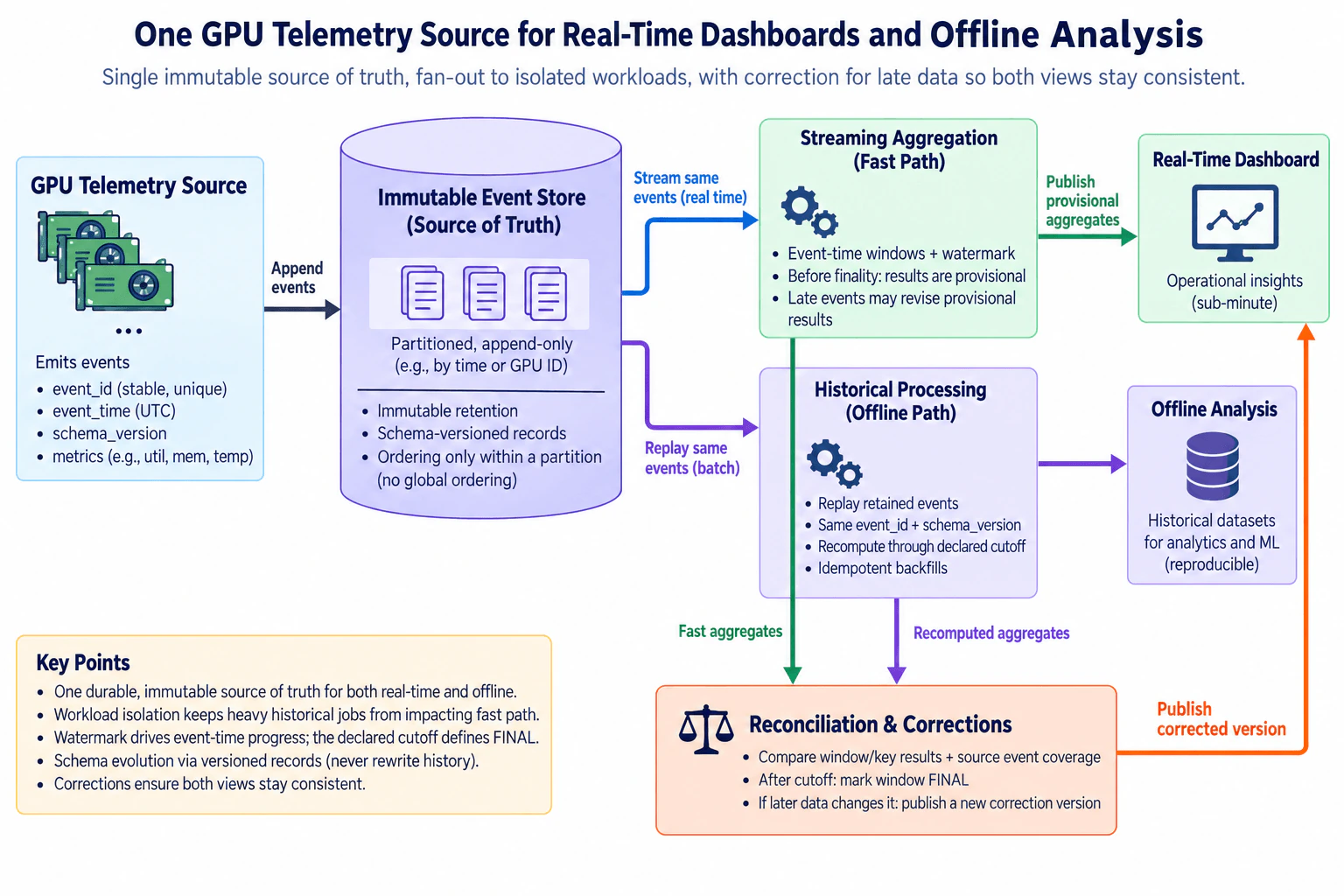
Design one durable source-of-truth path that feeds sub-minute operational aggregates and reproducible historical jobs. Specify fan-out boundaries, event identity, immutable retention, schema versions, watermark and finality, replay, correction publication, workload isolation, and reconciliation so the fast view and offline recomputation do not silently diverge.

Short Interview Answer (30-60 seconds)

I would append every GPU telemetry event to one durable, immutable event store and fan out from that shared history. The streaming path produces provisional sub-minute aggregates, while the offline path replays the same retained events for reproducible results. Stable event IDs, schema versions, event-time watermarks, a declared finality cutoff, idempotent backfills, workload isolation, and reconciliation keep both views aligned. The trade-off is extra storage and reconciliation work in exchange for reproducibility and safe corrections.

Detailed Explanation

The goal is to make one set of GPU measurements useful in two ways without creating conflicting histories. Operators need a very fresh dashboard, while analysts need results they can reproduce later. I would keep every original measurement in one durable history and let both uses read from it. The fast view can change as delayed measurements arrive. The historical view can recompute the same period later. A comparison step checks whether both paths agree and publishes a corrected version when they do not.

Useful Questions to Ask the Interviewer
  1. How late can telemetry normally arrive before a reporting window should be marked final?
  2. How long must the immutable telemetry history be retained for replay and backfills?
  3. When a finalized result changes, should consumers see a new correction version while retaining the earlier published version?
  4. What partition key should define the ordering scope that matters for GPU telemetry?
Use the same GPU telemetry source for real-time dashboards and offline analysis. diagram
How to Explain It in an Interview
1. Start with one durable GPU telemetry contract

I would make the Immutable Event Store the source of truth. The GPU Telemetry Source appends individual events containing a stable unique event_id, UTC event_time, schema_version, and telemetry metrics such as utilization, memory, and temperature. The store is append-only and retains historical records instead of rewriting old events when a schema changes. Records are partitioned, for example by time or GPU ID as shown in the design, and ordering is assumed only inside a partition, never globally. This gives both processing paths the same durable history.

2. Fan out into isolated real-time and offline workloads

The same retained history feeds two independent compute paths. Streaming Aggregation is the fast path for operational freshness. Historical Processing is the offline path for replay and reproducible analysis. The workloads are isolated, so a heavy historical replay or backfill does not have to consume the resources needed by the sub-minute path. Both paths still use the same source events and schema-versioned history, so isolation does not create a second source of truth.

3. Treat dashboard results as provisional

Streaming Aggregation uses event-time windows and a watermark. Event time is when the source measurement occurred. The watermark represents progress through event time; it is not permanent finality. Before the declared cutoff, results are provisional because late events may still revise them. The fast path publishes provisional aggregates to the Real-Time Dashboard for sub-minute operational insight. The stable event_id gives the design a consistent identity for reasoning about repeated or late events and for later reconciliation, without claiming any unsupported transport-level exactly-once guarantee.

4. Make historical recomputation replayable and deterministic

Historical Processing replays retained events using the same event_id and schema_version. A historical job recomputes results through a declared cutoff, so its input boundary is explicit. Backfills are idempotent, meaning rerunning the same historical range does not create duplicate logical results. Because the source history remains immutable, the job can reproduce the same input instead of depending on transient streaming state. The resulting historical datasets feed Offline Analysis for analytics and machine-learning work.

5. Reconcile the fast and recomputed views

Both processing paths feed Reconciliation & Corrections. The fast path sends its aggregates directly, and Historical Processing sends its recomputed aggregates directly. Reconciliation compares results by window and key and also compares source-event coverage, which helps detect missing or duplicated inputs that matching totals alone could hide. After the declared cutoff, the window is marked FINAL for publication purposes. If later data changes the correct answer, the design publishes a new correction version rather than silently pretending the earlier published result never existed.

6. Publish corrections directly to the dashboard

The correction path runs from Reconciliation & Corrections directly to the Real-Time Dashboard. Offline Analysis is not an intermediate publisher for dashboard corrections. This keeps the two consumer paths independent while allowing the real-time view to converge with the recomputed historical answer. The Offline Analysis dataset remains the reproducible historical output of Historical Processing, while the dashboard receives provisional fast aggregates and, when needed, a later corrected version.

7. Accept the freshness-versus-finality trade-off

The design intentionally separates freshness from finality. The dashboard receives useful results quickly, but those results may change. Waiting longer before marking a window final gives late events more time to arrive and reduces later corrections, but delays certainty. Immutable retention also costs storage, and replay plus reconciliation adds compute and operational work. We accept those costs because they provide reproducible historical jobs, safe backfills, workload isolation, and a concrete mechanism for detecting silent divergence between the fast and offline views.

Technical Approach
  1. Append each GPU telemetry event to the Immutable Event Store with stable event_id, UTC event_time, schema_version, and metrics.
  2. Keep the store partitioned and append-only, with ordering assumed only within a partition.
  3. Fan out the same retained events into Streaming Aggregation and Historical Processing.
  4. Use event-time windows and a watermark in the fast path and publish provisional aggregates to the Real-Time Dashboard.
  5. Replay retained events in Historical Processing through a declared cutoff and make backfills idempotent.
  6. Publish the historical result to Offline Analysis.
  7. Send fast aggregates and recomputed aggregates independently into Reconciliation & Corrections.
  8. Compare window/key results and source-event coverage.
  9. Mark a window FINAL after the declared cutoff.
  10. If later data changes the correct result, publish a new corrected version directly from Reconciliation & Corrections to the Real-Time Dashboard.
Practical Insights

The benefit is that one immutable history supports both low-latency dashboards and reproducible offline jobs, so the two paths are much less likely to silently disagree. The downside is extra storage because source events must be retained, plus extra compute for replay and reconciliation. Event-time processing also needs state for open windows and late data. A longer finality delay gives late events more time to arrive and can reduce later corrections, but users wait longer for certainty. Strong workload isolation protects the fast path from heavy backfills, but it requires separate capacity. We accept these costs because reproducibility, correction history, replay safety, and consistent results are more important than minimizing storage or operating only one compute path.

Why Interviewers Ask This

Interviewers ask this to test whether you can keep a fast streaming view and a slower historical view consistent when both come from the same underlying events. They want to see judgment around event identity, immutable retention, schema versions, partition-scoped ordering, event time, watermarks, late data, replay, idempotent backfills, workload isolation, finality, and reconciliation. The key skill is preventing two processing paths from becoming two conflicting sources of truth.

Common interview mistakes

Common mistakes are creating separate ingestion histories for real-time and offline use, treating a watermark as permanent finality, rewriting historical source events when schemas evolve, assuming global ordering across partitions, allowing large backfills to interfere with the fast path, publishing replay output non-idempotently, and comparing only aggregate totals without checking source-event coverage. Another mistake is routing dashboard corrections through the offline-analysis consumer. In this design, reconciliation receives both processing results directly and publishes corrected versions directly to the Real-Time Dashboard.

Interview tip

Lead with the invariant: one immutable event history feeds both paths. Then explain why the fast result is provisional, how the offline path replays the same events, and how reconciliation plus versioned corrections makes the dashboard converge with recomputation. Explicitly separate watermark from finality, and partition ordering from global ordering.

Interviewer may ask next
What would you change if historical backfills became so large that they started threatening the freshness of the real-time dashboard?

I would keep the same architecture and strengthen workload isolation rather than create another source of truth. The changed requirement is resource contention: Historical Processing now has enough replay load to threaten the sub-minute Streaming Aggregation path. The Immutable Event Store and event contract remain unchanged. Streaming Aggregation continues reading the same retained events and publishing provisional aggregates, while Historical Processing runs with separately bounded compute capacity so a large backfill cannot consume the resources needed by the fast path.

Correctness stays the same because both paths still use the same event_id, schema_version, and immutable history. Historical jobs still recompute through an explicit cutoff and remain idempotent. Reconciliation still compares fast and recomputed window/key results plus source-event coverage before any corrected version is published.

For recovery, I would slow or pause the historical replay instead of weakening the fast path. The replay can later resume from the same retained history. The downside is that large backfills may finish later and require more dedicated capacity, but operational freshness remains protected.

What happens if telemetry arrives after a window has already been marked FINAL?

I would keep the late event in the immutable source history and publish a new corrected version if it changes the correct result. The changed requirement is the publication state of a window that was already marked FINAL; ingestion does not change. The source event still carries its stable event_id, UTC event_time, and schema_version, and the original retained record is not rewritten.

Historical Processing can replay the affected retained events and recompute the window through the appropriate cutoff. Reconciliation compares the recomputed window/key result and source-event coverage with the previously published result. If the late event changes the answer, Reconciliation & Corrections publishes a new corrected version directly to the Real-Time Dashboard. Offline Analysis remains a separate historical consumer and is not used as an intermediate correction path.

Recovery stays deterministic because the historical path reads the same immutable history and backfills are idempotent. The downside is that consumers must understand versioned corrections even after a window was marked final.

8. How would you use cloud storage and managed data services while maintaining a strict security baseline?Cloud Data PlatformsEasyNvidia

Question Details

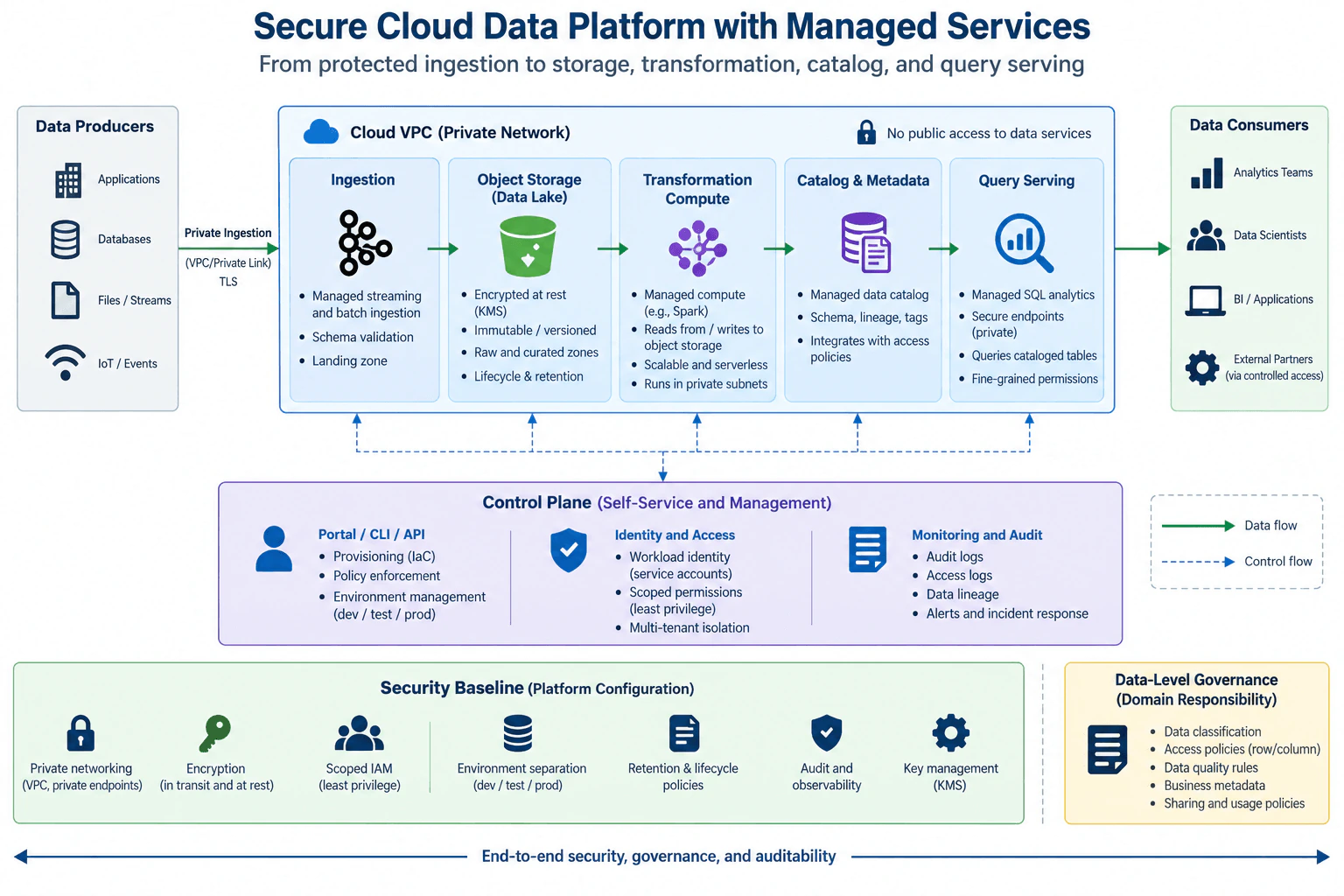
Design a basic data-platform path from protected ingestion to object storage, transformation compute, cataloged analytical tables, and query serving. Include private network paths, workload identity, encryption, scoped permissions, audit logs, environment separation, retention, and the boundary between platform configuration and data-level governance.

Short Interview Answer (30-60 seconds)

I would build a reusable private data platform with protected ingestion, encrypted object storage, managed transformation, a governed catalog, and private SQL serving. The platform team owns shared security controls, while domain teams own data-level governance. The trade-off is stronger isolation and enforcement versus more configuration and operational work.

Detailed Explanation

Producer teams need a repeatable way to move application, database, file, stream, and event data into analytics without rebuilding networking, identity, storage, and security for every workload. One-off pipelines make those controls inconsistent and harder to audit. I would provide a shared platform with protected ingestion, encrypted object storage, managed transformation, cataloged analytical data, and private query serving. The design keeps production records in the data plane and uses a separate control plane for provisioning, identity, policy, environment management, monitoring, and audit. Security defaults are centralized, while domain teams remain responsible for data-specific governance.

Useful Questions to Ask the Interviewer
  1. Which producer types are most important: applications, databases, files, streams, or event sources?
  2. Do consumers mainly need interactive SQL, BI access, data-science access, application access, or controlled partner access?
  3. What freshness and query-latency expectations matter for the analytical data?
  4. Which data classifications require row-level or column-level restrictions?
  5. How strong must isolation be between domains and between development, test, and production environments?
  6. What retention, deletion, and recovery expectations apply to raw and curated data?
  7. Are there existing workloads that must be migrated gradually into this platform?
How would you use cloud storage and managed data services while maintaining a strict security baseline? diagram
How to Explain It in an Interview
1. Start with the platform and security goals

The goal is a reusable cloud platform for multiple producer and consumer teams. The normal data path is protected ingestion to object storage, managed transformation, catalog and metadata, and then managed SQL query serving. Access to data services uses private network paths or private service endpoints rather than exposing the data services directly to the public internet.

The platform standardizes the controls every workload needs: encryption in transit and at rest, scoped identities and permissions, environment separation, retention policies, audit evidence, and observability. These are platform configuration responsibilities because they should be applied consistently across teams.

2. Define users and ownership

Producer teams supply data from applications, databases, files, streams, or events. They use the shared platform instead of building their own networking, storage, identity, and audit foundation.

Consumers include analytics teams, data scientists, BI or application users, and approved external partners using controlled access. They query or consume only through authorized serving interfaces.

The platform team owns the shared networking pattern, provisioning interfaces, workload-identity mechanisms, encryption and key-management configuration, environment separation, audit collection, and managed service configuration. Domain teams own classification, row and column access rules, data-quality rules, business metadata, and sharing or usage policies for their data.

3. Keep the control plane separate from production records

Teams use a portal, CLI, or API as the self-service entry point. Infrastructure as code provisions approved resources and applies policy defaults. The control plane also manages development, test, and production configuration.

Workloads receive dedicated workload identities with scoped permissions instead of shared credentials. The control plane also exposes monitoring, audit logs, access logs, lineage, alerts, incident-response signals, and operational status.

The dashed connections in the architecture represent control and policy flow. They do not carry business records. If a provisioning or policy operation fails, the requested configuration should not be promoted until that control-plane operation succeeds. Existing production data remains in the data plane.

4. Protect ingestion and land data in object storage

The first data-plane component is managed ingestion. It accepts supported streaming and batch inputs, performs schema validation, and writes accepted data into a landing area. The source connection uses encrypted transport over the protected ingestion path.

Object storage is the durable data-lake layer. It holds raw and curated zones, encrypts data at rest using the platform's key-management controls, and applies the configured versioning or immutability behavior together with lifecycle and retention policies.

If ingestion fails before data is committed to storage, the ingestion service or source-side delivery process owns retry or replay according to that source contract. The platform should expose the failure through logs and monitoring instead of silently treating partial delivery as success.

5. Transform data with managed compute

Managed transformation compute, such as a Spark-style managed engine, reads from object storage and writes transformed results back to object storage. The compute uses its own workload identity with least-privilege permissions and runs through the platform's private networking pattern.

Compute and storage are separate. If a transformation fails, retained source data can be used for recomputation instead of requiring producers to recreate the original input. A restarted job alone is not proof of recovery; the resulting curated data must be validated before it is published for consumers again.

The main trade-off is that managed compute reduces infrastructure ownership, but runtime configuration, permissions, dependency management, and cost still need operational controls.

6. Catalog metadata and serve governed analytical queries

The catalog stores metadata rather than production records. It describes schemas, lineage, tags, and logical table definitions and integrates with access policies. The physical analytical data remains in object storage.

Managed SQL analytics queries the cataloged tables through secure private access paths. Query serving returns results only to authorized consumers. Fine-grained permissions can restrict access at the dataset, row, or column level when the domain's governance policy requires it.

The normal data path is therefore producer to ingestion, ingestion to object storage, object storage through transformation, transformed output back to object storage, metadata publication into the catalog, cataloged analytical access through query serving, and results to authorized consumers.

7. Separate the strict security baseline from data-level governance

The security baseline is platform configuration. Private networking limits network exposure. Encryption protects data in transit and at rest. Scoped identity permissions restrict what each workload can access. Key management controls encryption keys. Development, test, and production remain separated so lower environments do not automatically share the same trust boundary as production. Retention and lifecycle policies control stored-object lifetime. Audit and observability record platform and data-access activity.

Data-level governance is a domain responsibility. The domain classifies its data, defines row or column access rules, owns data-quality policies and business metadata, and decides approved sharing and usage. This boundary matters because the platform can supply and enforce common mechanisms, but it cannot decide the business meaning or permitted use of every dataset.

Audit logs and access logs provide evidence of control-plane and data-access activity. Lineage helps identify where analytical data came from and which consumers may be affected by a data change. Alerts and incident-response signals help operators distinguish platform failures from domain-level data defects.

8. Handle reliability, adoption, cost, and trade-offs

Object storage is the main data recovery boundary shown in this design. When transformation output is wrong or a transformation job fails, the platform can recompute from retained input if the necessary source state is still available under the configured retention or versioning policy. The recovered output must be validated before consumers rely on it again.

The design does not claim automatic multi-region failover, a specific recovery objective, exactly-once processing, or a compliance guarantee because none of those requirements are supplied.

For adoption, I would move teams onto the same portal, CLI, API, identity model, environment model, and managed data path gradually. Existing workloads can be onboarded in small groups instead of requiring one large cutover.

Managed services reduce the infrastructure the platform team must operate, but they increase dependence on provider capabilities and policy models. Strong private networking, environment isolation, retention controls, and fine-grained authorization improve the security baseline but create additional configuration, operational effort, and cost. Shared services improve reuse, while stronger isolation reduces cross-team blast radius at the cost of more dedicated resources and administration.

Technical Approach
  1. Identify producer teams, consumer types, and the reusable analytical workloads the platform must support.
  2. Define the trust boundary: protected producer ingestion, private access to managed data services, and controlled consumer access.
  3. Separate the control plane from the production data plane. Put provisioning, identity, policy, environment management, monitoring, and audit in the control plane; keep business records in the data plane.
  4. Standardize protected ingestion for supported batch and streaming sources with encrypted transport and schema validation.
  5. Land data in encrypted object storage with raw and curated zones plus configured versioning or immutability, lifecycle, and retention behavior.
  6. Run managed transformation compute using workload identity and scoped permissions. Read from and write back to object storage through the private networking pattern.
  7. Register analytical metadata in the catalog, including schemas, lineage, tags, and links to access policies.
  8. Serve cataloged tables through managed SQL analytics using secure private access paths for authorized consumers.
  9. Apply platform-wide security controls: private networking, encryption, key management, least privilege, environment separation, audit logs, and observability.
  10. Keep domain-owned governance separate: classification, row and column access rules, data-quality rules, business metadata, and sharing policies.
  11. Use retained object data as the recomputation boundary when transformation fails, then validate recovered curated outputs before making them available again.
  12. Onboard workloads gradually through the common portal, CLI, API, and infrastructure-as-code path while monitoring adoption, reliability, operational burden, and cost without assuming fixed targets.
Practical Insights

The platform scales along several different boundaries. Ingestion capacity grows with producer traffic. Transformation capacity grows with the amount and concurrency of processing work. Object-storage usage grows with raw and curated retention. Catalog load grows with the number of datasets and metadata changes. Query capacity grows with consumer concurrency. Because storage and managed compute are separate, compute can change without moving the whole data lake. Private endpoints, encryption, audit logging, and fine-grained authorization add network, metadata, key-management, and operational work. Stronger separation between environments or tenants usually reduces blast radius but creates more resources and configuration to manage. Retaining more versions or history makes recomputation and recovery easier but increases storage cost. Managed services reduce infrastructure ownership, but storage, compute, requests, transfer, metadata operations, and operational support still affect cost. No exact throughput, latency, storage volume, migration duration, or cost is assumed.

Why Interviewers Ask This

Interviewers want to see whether I can design a reusable cloud data platform instead of only naming managed services. The main judgment is separating the production data path from the control plane while applying private networking, workload identity, encryption, least privilege, environment isolation, retention, audit evidence, and enforceable data-level governance at the correct boundaries.

Common interview mistakes

Common mistakes are treating the design as one ETL pipeline instead of a reusable platform; putting production records through the control plane; exposing data services publicly when private access is required; using shared credentials instead of workload identities; giving transformation or query services broad permissions; confusing catalog metadata with stored production data; assuming encryption or catalog tags alone provide authorization or compliance; mixing development, test, and production without an isolation boundary; ignoring lifecycle and retention; collecting logs without using them for access review and incident response; assigning business classification and row or column policy decisions entirely to the platform team; claiming a namespace alone provides tenant isolation; and claiming automatic failover, exactly-once behavior, or recovery objectives that were never defined.

Interview tip

Explain the design in two passes. First trace the production data path from protected ingestion to object storage, transformation, catalog, query serving, and consumers. Then trace the control path for identity, policy, environments, encryption, monitoring, and audit. Finish with the ownership boundary: platform teams provide enforceable controls, while domain teams define data-specific governance.

Interviewer may ask next
How would you change this platform if several domains required stronger isolation from each other?

I would keep the same ingestion, object-storage, transformation, catalog, and query pattern but strengthen the isolation boundaries instead of changing the normal data flow. Depending on the required risk separation, each domain could receive more dedicated identities, storage boundaries, key boundaries, network boundaries, or managed-compute boundaries. Development, test, and production would remain separated as well. The control plane would still provide the shared portal, CLI, API, infrastructure-as-code templates, policy enforcement, monitoring, audit collection, and status. Domain teams would still own classification and fine-grained data policies. The benefit is a smaller cross-domain blast radius and clearer authorization boundaries. The cost is more resources, configuration, operational support, and potentially lower sharing efficiency. I would choose the amount of dedicated infrastructure from the actual isolation requirement rather than assuming every domain needs complete physical separation.

What would you do if a transformation publishes incorrect curated data and consumers have already started querying it?

I would stop further publication of the incorrect result and use monitoring, lineage, audit evidence, and access information to identify the affected dataset and consumers. Object storage is the recovery boundary shown in this design. If the required source state is still available under the configured retention, versioning, or immutability behavior, I would correct the transformation and recompute the curated output from retained input. Restarting the task alone is not enough; the rebuilt data must be validated before consumers treat it as correct. The platform team owns the compute, storage, monitoring, and recovery mechanisms, while the domain owner validates business correctness and communicates the data impact to consumers. The design does not assume an automatic multi-region failover or a fixed recovery time.

9. Design the DGX telemetry lakehouse for five-second freshness and seven-day backfills.Cloud Data PlatformsMediumNvidia

Question Details

Choose durable messaging, stream compute, object storage, transactional table format, catalog, Spark and Trino access, and orchestration. Define partitions, file compaction, idempotent commits, schema registration, compute isolation, delayed-log replay, stable snapshots for readers, and monitoring of the five-second service level.

Short Interview Answer (30-60 seconds)

I would use Kafka, Flink, and Iceberg on object storage, with a REST catalog, isolated Spark and Trino compute, and Airflow for backfills and compaction. The main trade-off is five-second snapshot freshness versus higher commit, metadata, and small-file overhead.

Detailed Explanation

DGX nodes emit telemetry every five seconds, and consumers need new records to become queryable quickly while operators must still be able to replay delayed logs for seven days. A single streaming job is not enough because durability, schemas, transactional publication, historical replay, compaction, query isolation, and monitoring all need shared platform rules. I would use Kafka as the durable replay boundary, Flink for real-time processing, Iceberg on object storage as the publication boundary, a REST catalog for metadata, isolated Spark and Trino compute, and Airflow for bounded maintenance and recovery work.

Useful Questions to Ask the Interviewer
  1. What telemetry volume, device count, and peak event rate should the platform support?
  2. Is the five-second freshness target measured from device event time, platform arrival time, or Kafka arrival time to a queryable Iceberg snapshot?
  3. How much late or out-of-order telemetry is expected, and how long may event-time corrections remain open?
  4. What concurrency and isolation are required between streaming, Spark analytics, Spark backfills, and interactive Trino queries?
  5. Are there retention, authorization, or data-location requirements beyond the seven-day replay window?
Design the DGX telemetry lakehouse for five-second freshness and seven-day backfills. diagram
How to Explain It in an Interview
  1. Goals and service boundaries

The normal path is DGX telemetry producers to Kafka, Kafka to Flink, Flink to Apache Iceberg on S3-compatible object storage, and committed Iceberg snapshots to Spark and Trino through the Iceberg catalog. The recovery path is separate: Airflow triggers bounded Spark replay and compaction work. The five-second target is measured at the reader-visible publication boundary, not merely when Kafka receives an event or Flink processes it.

The seven-day requirement changes the source boundary. Kafka must retain telemetry for at least seven days so delayed logs can be replayed without depending on temporary Flink state. The design therefore treats Kafka as the durable replay source and the committed Iceberg snapshot as the durable table-publication boundary.

  1. Users, ownership, and reusable platform capabilities

DGX nodes are the producers. Their telemetry contract contains fields such as device_id, event_time, metric, value, and schema_version. The platform owns the shared Kafka, Schema Registry, Flink, Iceberg storage, catalog, Airflow, Spark, Trino, and monitoring capabilities. Spark users run analytics and bounded replay jobs. Trino users run interactive SQL. Operators watch freshness, lag, checkpoint health, commit failures, and compaction backlog.

The diagram does not show a separate portal, CLI, or provisioning service, so I would not invent one. The reusable platform surface is the common ingestion contract, registered schemas, shared transactional tables and catalog, isolated compute pools, and centrally orchestrated maintenance. Storage and metadata are shared platform services, while compute is isolated by workload so a large backfill does not directly consume the real-time Flink or interactive Trino compute pool.

  1. Durable ingestion and schema contracts

Kafka is the durable, replicated telemetry log. Producers use acks=all and idempotent producer behavior. Topics are partitioned by device_id so records for the same device preserve Kafka partition ordering. That ordering scope is per partition; it does not create a global order across all devices.

Kafka retention is at least seven days. This is the replay boundary for delayed telemetry and historical reprocessing. Retention alone does not make final table writes correct, so Flink and Spark still need deterministic deduplication or idempotent write logic.

Schema Registry stores registered and versioned telemetry schemas. It is contract metadata, not production telemetry storage. Records carry schema_version so current streaming and historical replay can interpret the same event according to the correct registered contract.

  1. Real-time processing with Flink

Flink consumes Kafka and performs event-time processing, validation, and deduplication. It keeps state using checkpoints and writes the validated result into Apache Iceberg. The design ties checkpoint-driven Iceberg commits to an interval no greater than the five-second freshness target.

That interval is a target-setting mechanism, not a guarantee by itself. End-to-end freshness also depends on Kafka lag, Flink processing time, checkpoint completion, Iceberg commit latency, and when the committed snapshot becomes visible to readers. If Flink falls behind, Kafka retains the input while monitoring exposes consumer lag and checkpoint health.

Flink runs in an isolated compute pool. This protects real-time processing from Spark analytics, Spark backfills, and Trino query concurrency. The trade-off is more compute boundaries to operate, but the blast radius of a heavy batch workload is smaller.

  1. Transactional lakehouse storage and partitions

Apache Iceberg is the transactional table format, and S3-compatible object storage holds Iceberg data files and metadata files. Iceberg creates atomic snapshots. Spark and Trino therefore read a committed table state rather than a mixture of old and partially written files.

The table uses the Iceberg partition transform hours(event_time). An optional bucket(N, device_id) transform can be added when device distribution and access patterns justify it. These are logical Iceberg partition transforms. Readers use Iceberg metadata rather than depending on a Hive-style directory naming convention in object storage.

Frequent commits help freshness but tend to create more metadata and smaller data files. Periodic compaction rewrites small files into larger files and publishes the rewrite as a new Iceberg snapshot. Readers can continue using a stable committed snapshot while the rewrite is in progress.

  1. Catalog and stable reader snapshots

The Iceberg REST catalog stores and serves table metadata, snapshot references, and the access-control metadata shown in the design. Production telemetry records remain in object storage, not in the catalog.

Spark and Trino resolve the table through the catalog and read committed Iceberg snapshots. Spark has an isolated compute pool for analytics and backfill jobs. Trino has an isolated compute pool for interactive SQL. Sharing the same Iceberg tables avoids copying data, while separate compute pools reduce noisy-neighbor effects.

The important consistency boundary is the Iceberg snapshot commit. Before a new snapshot commits, readers continue to see a previously committed state. After a successful commit, new readers can resolve the new committed snapshot. This is the stable-snapshot behavior the design needs for both Spark and Trino.

  1. Seven-day replay and idempotent backfills

Airflow orchestrates backfill and maintenance work. It does not transform telemetry itself. For delayed logs, Airflow triggers a bounded Spark replay job for up to seven days. Spark rereads the retained Kafka data, processes the requested range, and writes to the same Iceberg tables.

Replay writes must be idempotent. Re-running the same bounded range must not create duplicate final rows. The diagram represents this as merge or overwrite logic over bounded partitions and an idempotent new snapshot. A deterministic record identity or equivalent merge condition is therefore needed so the same input produces the same table result.

Backfill compute is isolated from the Flink streaming pool. If a replay consumes too much shared Kafka, network, or storage capacity, operators can throttle the replay rather than sacrificing the five-second streaming target. After the replay commits, the resulting Iceberg snapshot should be checked before the recovery is considered complete.

  1. Compaction and small-file control

The five-second target encourages frequent publication, which can produce many small files. Airflow schedules a separate compaction job that rewrites them into larger files. The compaction path writes a new Iceberg snapshot rather than mutating a reader-visible snapshot in place.

The monitoring system tracks compaction backlog. A growing backlog is an early warning that write frequency is creating file-layout pressure that may eventually hurt scan efficiency and increase metadata work.

  1. Monitoring the five-second service level

The primary freshness metric is end-to-end: event arrival to committed, queryable Iceberg snapshot. The target is five seconds. This metric matters more than an internal Flink processing timer because it measures the state consumers actually see.

Supporting signals identify where freshness is being lost. Kafka consumer lag shows ingestion or processing backlog. Flink checkpoint health shows whether streaming state and commit coordination are progressing. Iceberg commit failures show publication problems. Compaction backlog shows growing small-file pressure. Together these signals let operators distinguish broker, stream-compute, publication, and maintenance failures.

  1. Failure and recovery behavior

If Flink fails before a successful publication, Kafka remains the durable replay source and Flink recovers using its checkpointed state and source positions. A failed or incomplete table update must not be treated as a committed reader-visible result. The recovery boundary is therefore the last valid processing state plus the last committed Iceberg snapshot.

If a delayed source log arrives later, that is a replay or backfill, not merely a task retry. Airflow schedules Spark to reread the bounded historical range. The Spark job uses idempotent table writes and publishes a new snapshot. This distinction is important because restarting a failed task and recomputing seven days of historical data have different operational scopes and costs.

  1. Scaling and cost trade-offs

The first likely pressure points are Kafka partition capacity, Flink lag and checkpoint duration, Iceberg metadata and small-file growth, Spark replay contention, and Trino query concurrency. The design does not invent event rates or storage volumes, so capacity is increased from measured operational signals rather than assumed numbers.

Kafka can add partitions and broker capacity when ingestion or consumer parallelism becomes limiting. Flink can scale its processing parallelism while respecting key-based state and partition-ordering requirements. Spark replay capacity can scale independently from the real-time stream. Trino can scale for interactive concurrency without changing the storage layer.

The main trade-off is freshness versus write amplification and metadata pressure. Frequent Iceberg commits improve reader-visible freshness but increase snapshot activity and small-file production. Compaction reduces that pressure but consumes extra compute and object-storage operations. The second trade-off is shared storage efficiency versus isolated compute cost. Sharing Iceberg tables avoids copies, while separate Flink, Spark, and Trino pools reduce noisy-neighbor risk at the cost of operating more compute capacity.

  1. What this design deliberately does not claim

The design does not claim a specific device count, event rate, storage volume, recovery-time objective, recovery-point objective, or multi-region disaster-recovery guarantee because none is supplied. It also does not claim that a five-second checkpoint interval alone guarantees a five-second SLO. The service level is verified only at the committed, queryable Iceberg snapshot boundary.

Technical Approach
  1. Define the two hard boundaries: five-second reader-visible freshness and at least seven days of durable replay.
  2. Use Kafka as the durable telemetry log and replay source, with acks=all, idempotent producers, device_id partitioning, and retention of at least seven days.
  3. Register and version telemetry schemas separately from production records.
  4. Use Flink for event-time processing, validation, deduplication, checkpointed state, and transactional writes into Iceberg.
  5. Align checkpoint-driven Iceberg commits with the five-second target while measuring the actual SLO at the committed queryable snapshot boundary.
  6. Store Iceberg data and metadata files on S3-compatible object storage.
  7. Partition Iceberg with hours(event_time), with optional bucket(N, device_id) when justified by distribution and query patterns.
  8. Use the Iceberg REST catalog for table and snapshot metadata consumed by Spark and Trino.
  9. Isolate Flink streaming, Spark analytics and replay, and Trino interactive query compute.
  10. Use Airflow to orchestrate bounded seven-day Spark replays and periodic compaction; do not put transformation logic in Airflow.
  11. Make replay writes idempotent through deterministic merge or bounded overwrite behavior so repeating the same backfill does not duplicate final data.
  12. Compact small files periodically and publish the rewrite as a new Iceberg snapshot.
  13. Monitor event-arrival-to-queryable-snapshot freshness, Kafka lag, Flink checkpoint health, Iceberg commit failures, and compaction backlog.
Practical Insights

The design scales independently at several boundaries. Kafka capacity depends on producer throughput, partition count, retention, and replay traffic. Flink capacity depends on how quickly it can consume partitions, process state, finish checkpoints, and publish Iceberg commits. Object storage can grow separately from compute, but frequent Iceberg snapshots create metadata activity and many small files, which is why compaction matters. Seven-day Spark replays may read a large historical range, so their compute and concurrency are isolated from real-time Flink processing. Trino query concurrency scales separately from Spark and Flink. Network and object-storage work also increase during backfills and compaction. The design therefore watches lag, checkpoint health, commit failures, query contention, and compaction backlog before adding capacity. Cost grows with retained Kafka data, object storage, continuously running stream compute, isolated query pools, backfills, and compaction. No precise rate, storage size, or cost is assumed because the question does not supply one.

Why Interviewers Ask This

This question tests whether a candidate can connect a strict reader-visible freshness target with durable replay, transactional publication, workload isolation, and operational recovery. A strong answer separates messaging, stream compute, table transactions, metadata, query compute, orchestration, and monitoring instead of treating the system as one ETL job.

Common interview mistakes

Common mistakes include measuring five-second freshness only at Kafka or Flink instead of at the committed queryable Iceberg snapshot; treating Kafka delivery as proof of end-to-end exactly-once correctness; retaining less than seven days of replayable input; using Airflow as the transformation engine rather than the orchestrator; letting Spark backfills compete directly with latency-sensitive Flink compute; writing non-idempotent replays that duplicate final rows; assuming object-store directory names define Iceberg partitions; skipping compaction despite frequent small-file-producing commits; confusing the Iceberg catalog with production data storage; reversing the catalog or reader flow; and claiming that a five-second checkpoint interval alone guarantees the service-level target.

Interview tip

Organize the answer around two durable boundaries: Kafka is the seven-day replay boundary, and a committed Iceberg snapshot is the reader-visible publication boundary. Trace the normal path first, then the Airflow-and-Spark replay path, and finish with compute isolation, small-file compaction, and the metrics that prove the five-second target.

Interviewer may ask next
What would you do if a seven-day Spark backfill starts hurting the five-second freshness target?

I would keep the same architecture and protect the real-time path with the compute isolation already shown. Flink continues in its dedicated streaming pool, while Spark backfills run in a separate bounded pool. I would limit backfill concurrency and process explicit replay ranges instead of allowing unlimited historical work. I would watch end-to-end freshness, Kafka lag, Flink checkpoint health, and Iceberg commit failures. If the backfill is saturating a shared dependency such as Kafka, network bandwidth, or object storage, I would throttle the backfill before weakening the streaming target. The trade-off is a longer backfill completion time in exchange for protecting current telemetry freshness.

How would you handle a schema change while seven-day-old telemetry is still being replayed?

I would use the registered and versioned telemetry schemas as the contract boundary and keep schema_version on each record. Flink validates current records against the matching registered version, and the Spark replay path resolves historical records using the same versioned contract. Compatible schema changes can be evolved into the Iceberg table when the table schema supports them. An incompatible change should be rejected or handled through an explicit schema-evolution step rather than silently reinterpreting old telemetry. Iceberg keeps readers on a stable committed snapshot while the replay is running. After the backfill publishes a new snapshot, I would verify validation results and the resulting table state before marking the replay complete.

10. Design a lakehouse platform for five million GPU events per second and under-five-minute queries.Cloud Data PlatformsHardNvidia

Question Details

Choose regional ingestion, messaging partitions, streaming compute, transactional object-store tables, metadata and commit services, compaction, query engines, and dashboard aggregates. Preserve exactly-once business results, two-hour-late events, hot GPU keys, schema evolution, replay, workload isolation, disaster recovery, and measurable cost at sustained and burst load.

Short Interview Answer (30-60 seconds)

I would use regional Kafka ingestion, Flink event-time processing, transactional Iceberg tables on object storage, and Trino with isolated dashboard and backfill workloads. The main trade-off is extra compute and operational work for salting, aggregates, compaction, and standby capacity in exchange for predictable correctness, freshness, and recovery.

Detailed Explanation

GPU servers, inference clusters, AI services, and other systems continuously produce telemetry that must be queryable within five minutes at five million events per second. A single pipeline is not enough because the platform must support many producers and consumers while also handling two-hour-late events, duplicate delivery, replay, hot GPU keys, schema evolution, maintenance, workload contention, and regional failures. I would build reusable ingestion, streaming, transactional storage, metadata, query, recovery, and cost-measurement capabilities. The design prioritizes correct business results and stable dashboard freshness while keeping sustained load, burst load, storage work, query work, and disaster-recovery capacity visible.

Useful Questions to Ask the Interviewer
  1. What recovery objectives should apply to a regional failure, and how much temporary query degradation is acceptable during failover?
  2. How long must Kafka data remain available for replay beyond the required two-hour late-event window?
  3. What query concurrency should dashboard traffic and ad-hoc or backfill workloads expect?
  4. Which schema changes are considered compatible, and which changes require a controlled migration?
  5. Should disaster-recovery compute remain continuously provisioned or be activated only during an incident?
Design a lakehouse platform for five million GPU events per second and under-five-minute queries. diagram
How to Explain It in an Interview
1. Goals and constraints

The normal production path is GPU event producers to regional Kafka, then Flink, Iceberg tables on object storage, Trino, and finally dashboards, analysts, and downstream data products. The fixed throughput is five million events per second with burst headroom, and dashboard queries must remain under five minutes. The same design must preserve correct results when events arrive late, are delivered more than once, or are replayed.

The likely first ingestion bottleneck is partition skew, not only total broker throughput. A few GPU identifiers can become disproportionately hot. The Kafka layer therefore uses many partitions and a salted partition expression, HASH(GPU_ID, SALT_BUCKET), to spread a single hot GPU across multiple partition buckets. Kafka retention is kept long enough for the required replay window instead of assuming an arbitrary fixed number of days.

2. Users and ownership

The producer boundary includes GPU servers used for training, GPU inference clusters, AI platforms and services, and other system, metric, or log sources. Producers own the meaning of their events and the fields needed for correct processing, including stable event identifiers, GPU identifiers, event timestamps, and compatible schemas.

The shared platform owns regional Kafka ingestion, Flink streaming execution, Iceberg storage, the Iceberg REST Catalog metadata and commit path, asynchronous compaction and snapshot maintenance, Trino serving, replay mechanics, cross-region recovery capability, workload isolation, and cost measurement.

Consumers are near-real-time dashboards, analysts using SQL, and applications or data products. The final diagram does not define a separate portal, CLI, API, or provisioning workflow, so I would not claim a self-service control plane that is not shown. Teams consume the reusable platform capabilities through the shared ingestion, table, catalog, and query boundaries visible in the architecture.

3. Data plane and metadata boundary

Production event records stay in the data plane. Kafka carries event records into Flink. Flink processes them and publishes transactional table changes into Iceberg-backed object storage. Trino reads those Iceberg tables and returns query results to consumers.

The Apache Iceberg REST Catalog is a metadata and commit service, not another production-record store. It maintains table metadata, atomic commit coordination, snapshots and time-travel information, schema evolution, partition evolution, namespaces, and the access-control information represented in the architecture. Flink and Trino use this metadata path to resolve and update table state. A catalog failure can block new commits or table discovery without turning catalog traffic into the event-data path.

4. Regional Kafka ingestion and hot-key control

Regional Kafka clusters absorb sustained traffic and bursts. The architecture uses many partitions to create parallel ingestion capacity. Each representative partition uses HASH(GPU_ID, SALT_BUCKET), which deliberately breaks the one-GPU-to-one-partition assumption for hot GPUs.

That improves load distribution, but it introduces a trade-off: downstream processing cannot depend on all records for one GPU being naturally serialized in a single Kafka partition. Any GPU-level aggregation that needs a unified result must merge the salted substreams correctly in Flink.

Kafka also retains the source event log for replay. Replay is a recovery or recomputation path, not the ordinary query path. Retention must therefore cover the operational replay requirement rather than being chosen only for storage convenience.

5. Flink event-time processing and exactly-once business results

Flink performs event-time processing and uses a two-hour watermark policy so events can arrive substantially later than their original event timestamp. The streaming logic deduplicates or upserts by event ID, which is essential when records are retried or replayed.

The diagram's exactly-once claim applies to the business-result boundary formed by Flink checkpointing plus transactional sink publication. It should not be interpreted as 'Kafka delivered every record exactly once.' Transport retries can still produce repeated input delivery. Correctness comes from recoverable Flink state, deterministic event handling, event-ID deduplication or upsert behavior, and transactional Iceberg publication.

Skew-aware key salting and rebalancing distribute work from hot GPUs across processing capacity. Operators observe consumer lag, checkpoint health, watermark progress, backpressure, state growth, restart activity, and sink commit failures to determine whether the stream is keeping up.

6. Transactional Iceberg storage

The lakehouse contains raw or detail GPU-event tables and dashboard aggregate tables. Physical Parquet files live in object storage. Apache Iceberg supplies the transactional table layer above those files.

The detail tables preserve GPU events and are partitioned by dimensions such as time and entity, matching the architecture. They retain the detailed history needed for SQL analysis, downstream products, validation, and replay reconciliation.

Dashboard aggregate tables contain pre-aggregated data intended for roughly one-to-five-minute query access. This prevents every dashboard refresh from scanning the complete raw history. The trade-off is additional streaming compute and storage in exchange for lower query work and more predictable freshness.

Iceberg snapshots provide an atomic publication boundary for readers. Schema evolution and partition evolution are controlled through table metadata, allowing the platform to change logical schema or physical organization without treating every compatible change as a full table replacement.

7. Metadata and commit service

The Iceberg REST Catalog coordinates table metadata and commits between engines. It records logical table state separately from the Parquet production records stored in object storage.

This boundary matters because multiple engines must agree on the current table snapshot. Flink uses it while publishing table updates, and Trino uses it while resolving tables and snapshots for reads. Atomic metadata publication prevents consumers from observing a partially published table state.

A catalog or commit-service outage mainly affects new table commits and table discovery. Recovery must restore or fail over catalog metadata consistently with the corresponding object-storage state before writers and readers resume normal operation.

8. Asynchronous compaction and maintenance

High-rate streaming writes can create many small files. The separate Compaction & Maintenance service rewrites small files and expires snapshots asynchronously. Its work is intentionally non-blocking relative to the latency-critical streaming path.

Running compaction inline with every streaming commit would couple ingest latency to file-rewrite throughput. Separating it keeps ingestion responsive, but it creates another operational queue that must be measured. Operators should track file counts, file sizes, snapshot growth, maintenance backlog, object-store requests, and compaction compute.

If compaction falls behind, ingestion can continue, but query efficiency may gradually degrade because Trino must open and scan a less efficient file layout. The recovery action is to restore maintenance capacity and reduce backlog rather than stopping the production event stream unnecessarily.

9. Trino serving and workload isolation

Trino serves SQL over the Iceberg tables. The architecture separates high-priority dashboard queries from ad-hoc and backfill queries using distinct workload queues or resource groups.

This isolation protects the under-five-minute dashboard objective from large historical scans. When capacity is constrained, lower-priority ad-hoc or backfill work can wait while dashboard queries receive the preferred share of query resources.

The important operational signals are dashboard and backfill queue depth, query latency, CPU consumption, scan bytes, concurrency, and failures. Workload isolation does not eliminate shared-resource limits, so admission control and queueing remain necessary when total demand exceeds available capacity.

10. Consumer interfaces

Near-real-time dashboards read the pre-aggregated tables through Trino. Analysts use SQL for interactive investigation. Applications and downstream data products can also consume governed lakehouse tables or query results through the same serving boundary represented in the architecture.

The platform does not invent an additional cache, API service, warehouse, or serving database. The selected design deliberately keeps the consumer path on Trino and Iceberg so that the written answer remains consistent with the approved diagram.

Consumer-visible freshness depends on several boundaries working together: Kafka lag, Flink watermark and checkpoint progress, successful Iceberg commits, aggregate-table updates, table maintenance, and Trino queue latency. A stale dashboard therefore needs diagnosis across those boundaries rather than being treated as only a query-engine problem.

11. Replay and reconciliation

Replay begins from retained Kafka data and feeds records back into Flink. It is used after processing corrections, recovery, or controlled recomputation. Because replayed input may contain events already represented in Iceberg, the event ID remains the business deduplication key.

Flink restores processing state or reprocesses retained events, and transactional Iceberg publication prevents partially committed table changes from becoming visible. Operators reconcile event counts, commit state, late-event behavior, raw-table results, and dashboard aggregates before declaring the replay complete.

Replay is different from retry. A retry repeats a failed operation near its original boundary. Replay intentionally reprocesses a retained range of historical events. It is also different from disaster-recovery failover, which moves service execution to the secondary-region capacity.

12. Cross-region disaster recovery

The disaster-recovery design replicates object storage and catalog metadata to a secondary region. It also maintains standby Kafka, Flink, and Trino capacity. During a regional failure, the platform can fail over to the standby services or replay from retained Kafka or durable object-storage data when required.

Recovery order is important. The secondary region first needs consistent durable table data and catalog metadata. The ingestion and streaming boundary can then restore state or replay retained events. Trino should resume serving after the recovered catalog and table snapshots are usable.

The design does not invent an RPO or RTO. Those objectives must come from the business. They determine how much data replication, metadata protection, Kafka retention, and standby compute capacity the platform should pay for.

13. Cost measurement at sustained and burst load

Cost is measured at the same boundaries that scale. In ingestion, meter events and bytes entering Kafka and the retention footprint. In streaming, measure Flink compute. In storage, measure object-store bytes and requests. Measure compaction compute separately because maintenance can rise after a burst. In serving, measure Trino CPU and scan bytes.

The architecture also tracks cost by tenant, workload, and environment where those attribution dimensions exist. That makes burst behavior visible. A traffic spike can raise Kafka, Flink, object-store, compaction, and later query costs at different times rather than producing one unexplained platform total.

The major cost trade-offs are explicit. More Kafka partitions and Flink capacity improve throughput headroom. Dashboard aggregates spend extra compute and storage to reduce repeated scans. Continuous compaction spends background compute to protect query efficiency. Workload isolation reserves capacity for important queries. Cross-region standby services improve recovery readiness but add capacity cost even while the primary region is healthy.

14. Reliability and failure handling

Kafka failures are observed through broker health, partition availability, consumer lag, and retention pressure. Flink failures are observed through checkpoint failures, restart activity, backpressure, watermark delay, and state growth. Iceberg and catalog failures appear as commit errors, metadata access problems, or snapshot-publication failures. Trino failures appear through queue growth, query errors, latency, CPU pressure, and scan volume.

The blast radius should follow the failing component. A streaming-job problem does not automatically make historical Iceberg data unavailable. A compaction backlog does not necessarily stop ingestion. A Trino saturation event should not corrupt streaming publication. A producer publishing bad event semantics is a data-product defect rather than proof that the shared platform itself is down.

After recovery, the platform validates committed snapshots, record counts, replay boundaries, late-event processing, aggregate results, query availability, and cost signals before returning to normal operation.

15. Schema evolution and controlled change

Schema evolution is handled through Iceberg metadata and producer compatibility rules. Partition evolution allows the physical organization of a table to change as query and data patterns change.

The architecture does not define a separate deployment portal or migration service, so I would not invent one. For a breaking data change, I would use the capabilities already present: publish the new schema or table state, use replay or backfill where historical data must be regenerated, reconcile old and new results, move consumers, and then retire the old representation after validation.

This avoids an all-at-once rewrite while staying inside the diagram's Kafka, Flink, Iceberg, catalog, replay, and query boundaries.

16. Final trade-offs

Salted Kafka partitioning reduces hot-key concentration but makes GPU-level aggregation more complex. A two-hour event-time window improves late-data correctness but increases streaming state and recovery work. Pre-aggregated dashboard tables improve query freshness but consume additional streaming compute and storage. Object storage keeps durable history economical relative to a dedicated high-performance copy, but streaming small files require compaction.

Separate Trino queues protect dashboards but can increase waiting time for ad-hoc and backfill work. Asynchronous compaction protects the ingest path but can temporarily allow less efficient file layouts. Cross-region standby capacity improves disaster recovery but increases steady-state cost. The design is therefore intentionally balanced around correctness and predictable freshness rather than minimizing every infrastructure component.

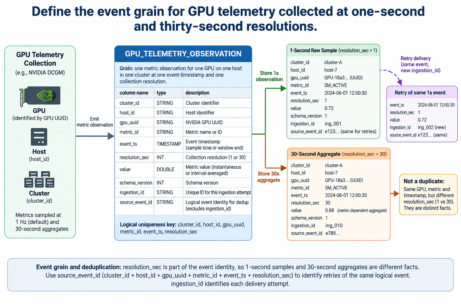
Technical Approach
  1. Fix the requirements first: five million GPU events per second, burst headroom, under-five-minute dashboard queries, two-hour-late events, exactly-once business results, replay, hot keys, schema evolution, workload isolation, disaster recovery, and measurable cost.
  2. Define the producer and consumer boundaries shown in the architecture.
  3. Use regional Kafka as the retained ingestion layer with many partitions.
  4. Partition hot GPU traffic with HASH(GPU_ID, SALT_BUCKET) so one GPU cannot dominate a single partition.
  5. Process events in Flink using event time, a two-hour watermark policy, event-ID deduplication or upsert, skew-aware salting, checkpointing, and transactional sink publication.
  6. Write raw or detail tables and dashboard aggregate tables as Apache Iceberg tables backed by Parquet files in object storage.
  7. Keep the Iceberg REST Catalog as the metadata and atomic-commit coordination boundary instead of putting production records in the catalog.
  8. Run compaction and snapshot maintenance asynchronously so small-file cleanup does not block ingestion.
  9. Serve SQL through Trino and isolate high-priority dashboard queries from ad-hoc and backfill queues.
  10. Use retained Kafka data as the explicit replay source and reconcile replayed outcomes through event IDs and committed Iceberg snapshots.
  11. Replicate object storage and catalog metadata across regions and keep standby Kafka, Flink, and Trino capacity for failover or recovery.
  12. Meter ingestion, retention, streaming compute, object-store usage and requests, compaction, Trino CPU, and scan bytes at sustained and burst load.
  13. Observe lag, checkpoints, watermark progress, commit health, maintenance backlog, query queues, latency, and recovery validation.
Practical Insights

The supplied event rate puts pressure on Kafka partitions, network throughput, Flink parallelism, checkpoint state, table commits, file creation, and downstream query work. Many Kafka partitions provide parallelism, while salted GPU keys prevent a few hot GPUs from concentrating traffic in one partition. The two-hour event-time window can increase the amount of Flink state that remains active. Longer Kafka retention improves replay capability but consumes more broker storage. Streaming writes create many files, so Iceberg needs asynchronous compaction. Dashboard aggregates reduce repeated scans but cost extra streaming compute and object storage. Trino workload isolation protects dashboard latency by allowing backfills to queue separately. Cross-region replication and standby Kafka, Flink, and Trino improve recovery but increase ongoing capacity cost. The platform therefore meters events and bytes in, Kafka retention, Flink compute, object-store bytes and requests, compaction compute, Trino CPU, and scan bytes instead of relying on one total cost number.

Why Interviewers Ask This

This question tests whether a Data Engineer can turn extreme streaming scale into a reusable lakehouse platform with clear correctness, storage, metadata, serving, isolation, recovery, and cost boundaries. The key judgment is separating transport delivery from correct business results while keeping dashboard freshness predictable under sustained load, bursts, late data, replay, hot keys, maintenance, and failures.

Common interview mistakes

Common mistakes include partitioning only by GPU_ID when a few GPUs can become hot; assuming Kafka delivery alone creates exactly-once business results; ignoring the two-hour event-time requirement; allowing replay to duplicate already committed outcomes; storing production event payloads in the catalog instead of object storage; forgetting that streaming writes generate small files; running compaction synchronously on the ingestion path; making dashboard queries compete directly with large backfills; claiming schema evolution without a transactional table and metadata boundary; confusing retry, replay, failover, and recomputation; assuming object-storage replication alone provides disaster recovery; inventing an RPO or RTO; and measuring only storage cost while ignoring Kafka retention, Flink compute, compaction, object-store requests, Trino CPU, scan bytes, and standby capacity.

Interview tip

Explain the normal path left to right first. Then explain the metadata path, replay path, compaction path, and disaster-recovery path separately. Tie each choice to a requirement: salted Kafka partitions for hot keys, Flink event time for late events, Iceberg transactions for atomic publication, Trino workload queues for dashboard isolation, and boundary-level metering for cost.

Interviewer may ask next
What would you change if dashboard concurrency increased sharply while ingestion remained at five million events per second?

I would keep the Kafka, Flink, Iceberg, and catalog architecture unchanged and scale the existing serving boundary. Dashboard aggregate tables would remain the preferred source because they avoid repeatedly scanning detailed history. I would add Trino capacity to the high-priority dashboard resource group while keeping ad-hoc and backfill queries in their separate lower-priority queue. I would watch dashboard queue depth, query latency, CPU, scan bytes, and file layout. If scans are still too expensive, I would adjust the existing aggregate grain and compaction behavior rather than introduce a new serving system that is not part of the approved architecture. The trade-off is more query and aggregation cost in exchange for protecting dashboard freshness.

How would the platform recover if the primary region failed while Flink still had work that had not been committed to Iceberg?

I would recover durable dependencies before allowing new writes. The secondary region first needs the replicated object-store data and catalog metadata represented in the architecture. Standby Kafka, Flink, and Trino capacity can then take over. Flink work that never reached a committed Iceberg snapshot is not treated as published business output. Flink restores recoverable processing state or replays retained Kafka records. Event-ID deduplication or upsert logic and transactional Iceberg publication prevent recovered processing from creating duplicate committed results. Trino resumes after the recovered catalog and tables are consistent. Operators then reconcile snapshot state, event counts, late-event handling, raw tables, and dashboard aggregates before declaring recovery complete. The design does not invent an RPO or RTO; those remain business inputs.

More questions load as you scroll

Disclaimer: This interview guide is for educational and informational purposes only. It is designed to help readers prepare, but it does not guarantee any interview result, hiring decision, offer, or outcome. Interview questions, hiring criteria, and preferred answers can vary by employer, interviewer, industry, location, and time. The examples and explanations reflect the authors' research and judgment, are provided without warranties of any kind, and should not be treated as the only correct approach. Diagrams are simplified illustrations intended to highlight the main components and their interactions; actual systems and implementations may be more complex. Alternative approaches may be equally valid or better suited to a particular question, context, or interviewer. To the fullest extent permitted by applicable law, the author, contributors, and publisher are not liable for decisions made, actions taken, or losses incurred based on this guide.

Company Notice: This guide is an independent educational resource and is not affiliated with, endorsed by, sponsored by, or approved by the company named in this guide. Company names are used only to identify interview experiences commonly reported by candidates. Interview practices can change without notice, and inclusion of company-specific content does not mean these questions are official, complete, or guaranteed to be asked. To the fullest extent permitted by law, the author, contributors, and publisher are not responsible for outcomes related to use of this material.

Content Accuracy and Verification: To the fullest extent permitted by applicable law, we do not represent or warrant that interview guides, questions, answers, examples, or diagrams are accurate, complete, current, error-free, or suitable for any particular purpose. You are responsible for independently reviewing and verifying the information before relying on it.