15 Meta Data Engineer Interview Questions & Answers

meta icon

Questions with Detailed ExplanationsWith Detailed Explanations

(Last Updated: September 8, 2026)

1. Define the fact-table grain and dimensions for Reels engagement reporting.Data ModelingEasyMeta

Question Details

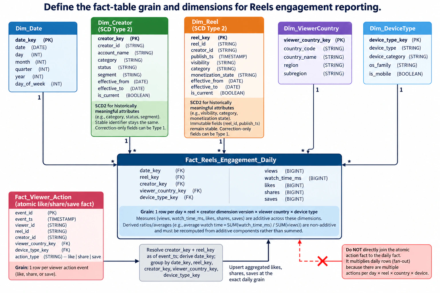
Support views, watch_time_ms, likes, shares, and saves sliced by creator, viewer country, device type, and day. Choose the row grain, identify which creator and reel attributes need slowly changing dimensions, distinguish additive from non-additive measures, and prevent a viewer action fact from being multiplied by daily summary rows.

Short Interview Answer (30-60 seconds)

I would use one daily row per day, reel, creator SCD version, viewer country, and device type. Views, watch time, likes, shares, and saves are additive. Creator and reel history uses SCD Type 2. Individual viewer actions must be aggregated to that exact daily grain before loading.

Detailed Explanation

This question asks how to organize Reels activity so reports give correct numbers by creator, country, device, and day. First, decide exactly what one stored daily row represents. Next, keep creator and reel details in separate records so older reports can still show the values that were true at the time. The stored numbers must also combine safely when reports cover several days or groups. Finally, individual likes, shares, and saves must be summarized before they are combined with daily totals, or the same daily numbers could be repeated and counted more than once.

Useful Questions to Ask the Interviewer
  1. Should historical reports use the creator and reel attributes that were valid when the engagement happened, or always show their current attributes?
  2. What reporting-day timezone should be used when deriving date_key from event_ts?
  3. Are viewer country and device type standardized before data reaches the reporting model?
  4. Can like, share, or save events be reversed or corrected after they arrive?
Define the fact-table grain and dimensions for Reels engagement reporting. diagram
How to Explain It in an Interview

Start with the grain. Fact_Reels_Engagement_Daily has exactly one row per date_key × reel_key × creator_key × viewer_country_key × device_type_key. Because creator_key and reel_key are surrogate keys for SCD Type 2 dimensions, the grain includes the historical creator and reel versions that apply to that reporting period.

The daily fact contains five foreign keys: date_key, reel_key, creator_key, viewer_country_key, and device_type_key. Its measures are views, watch_time_ms, likes, shares, and saves. These five stored measures are additive across the dimensions shown, so they can be summed when reporting across days, reels, creators, countries, or devices.

Dim_Date contains date_key, date, day, month, quarter, year, and day_of_week. Dim_ViewerCountry contains viewer_country_key, country_code, country_name, region, and subregion. Dim_DeviceType contains device_type_key, device_type, device_category, os_family, and is_mobile. These tables hold descriptive attributes used for slicing instead of placing those descriptions directly in the fact.

Dim_Creator is SCD Type 2. creator_key is its surrogate primary key, while creator_id is the stable business identifier. Historically meaningful attributes such as account_name, category, status, and segment create a new dimension version when they change. effective_from, effective_to, and is_current identify the period for each version. Stable identifiers remain unchanged, while correction-only attributes can be updated as Type 1 when old values do not need to be preserved.

Dim_Reel is also SCD Type 2. reel_key is its surrogate primary key and reel_id is its stable business identifier. Historically meaningful changing attributes include visibility, category, and monetization_state. The immutable fields reel_id and publish_ts remain stable. effective_from, effective_to, and is_current identify each historical reel version. Correction-only fields can be handled as Type 1 when historical preservation is unnecessary.

The separate Fact_Viewer_Action table is an atomic event fact for likes, shares, and saves. Its grain is one viewer action event per row. It contains event_id, event_ts, viewer_id, reel_id, creator_id, viewer_country_key, device_type_key, and action_type.

Before viewer actions contribute to the daily fact, resolve creator_key and reel_key to the SCD Type 2 versions valid as of event_ts, derive date_key, and group by date_key, reel_key, creator_key, viewer_country_key, and device_type_key. Then upsert the aggregated likes, shares, and saves into Fact_Reels_Engagement_Daily at that exact grain.

Do not directly join Fact_Viewer_Action to Fact_Reels_Engagement_Daily when calculating reporting metrics. Several viewer action rows can correspond to one daily summary row. A direct join would repeat that daily row once for each matching action, which can multiply views, watch_time_ms, or other already-aggregated values. Aggregating the atomic actions first prevents that fan-out.

The five stored measures are additive, but derived ratios and averages are non-additive. For example, average watch time should be calculated from the additive components as SUM(watch_time_ms) / SUM(views) at the requested reporting level. Do not sum previously calculated averages.

The main tradeoff is detail versus reporting efficiency. The daily fact is efficient for common reporting because it stores already-aggregated measures at a declared grain. The atomic viewer-action fact keeps event-level like, share, and save detail. Keeping the two grains separate preserves detailed events while preventing event rows from multiplying daily summary measures.

Technical Approach
  1. Declare the daily fact grain as date_key × reel_key × creator_key × viewer_country_key × device_type_key.
  2. Resolve creator_id and reel_id to the SCD Type 2 surrogate-key versions valid as of event_ts.
  3. Derive date_key from event_ts using the agreed reporting-day rule.
  4. Group individual like, share, and save events by the exact five daily fact keys.
  5. Upsert the aggregated likes, shares, and saves into the matching Fact_Reels_Engagement_Daily row.
  6. Sum additive stored measures for reporting.
  7. Recompute ratios and averages from additive components instead of summing derived values.
  8. Never directly join the atomic action fact to the daily summary fact for metric aggregation.
Practical Insights

The daily table makes reporting cheaper because many individual events have already been summarized into one row for each reporting combination. The extra cost is in the data-loading process: it must find the correct historical creator and reel versions, group action events, and update the matching daily rows. SCD Type 2 also stores multiple versions when creator or reel attributes change. The atomic action table uses more storage because it keeps individual events, but it preserves detail for event-level analysis.

Why Interviewers Ask This

This tests whether the candidate can define a precise reporting grain, choose appropriate dimensions and measures, preserve historical creator and reel attributes, distinguish additive measures from derived metrics, and prevent join fan-out from corrupting analytical results.

Common interview mistakes

Common mistakes include choosing an unclear fact grain; storing creator, country, or device descriptions directly in the fact; using creator_id or reel_id without resolving the correct SCD Type 2 version; forgetting viewer_country_key or device_type_key when aggregating atomic actions; summing derived averages such as average watch time; directly joining viewer-action events to daily summary rows and multiplying measures; and combining facts before both sources are at the same grain.

Interview tip

State the grain first, then explain the dimensions, SCD Type 2 history, additive measures, and the fan-out failure case. Emphasize that individual viewer actions are first transformed to exactly the same daily grain before their measures are loaded into the summary fact.
Interviewer may ask next
How would you calculate average watch time correctly across several days or creators?

Do not sum or average precomputed row-level averages. Keep watch_time_ms and views as additive components, then calculate the requested value as SUM(watch_time_ms) / SUM(views) after filtering and grouping at the requested reporting level. This correctly weights rows with different view counts.

How do you assign a viewer action to the correct creator and reel SCD Type 2 versions?

Use creator_id and reel_id as business identifiers and use event_ts to find the creator and reel records whose effective periods apply at that time. Take their creator_key and reel_key surrogate keys, derive date_key, and then aggregate with viewer_country_key and device_type_key before loading the daily fact.

2. Design a schema for analyzing process execution time.Data ModelingEasyMeta

Question Details

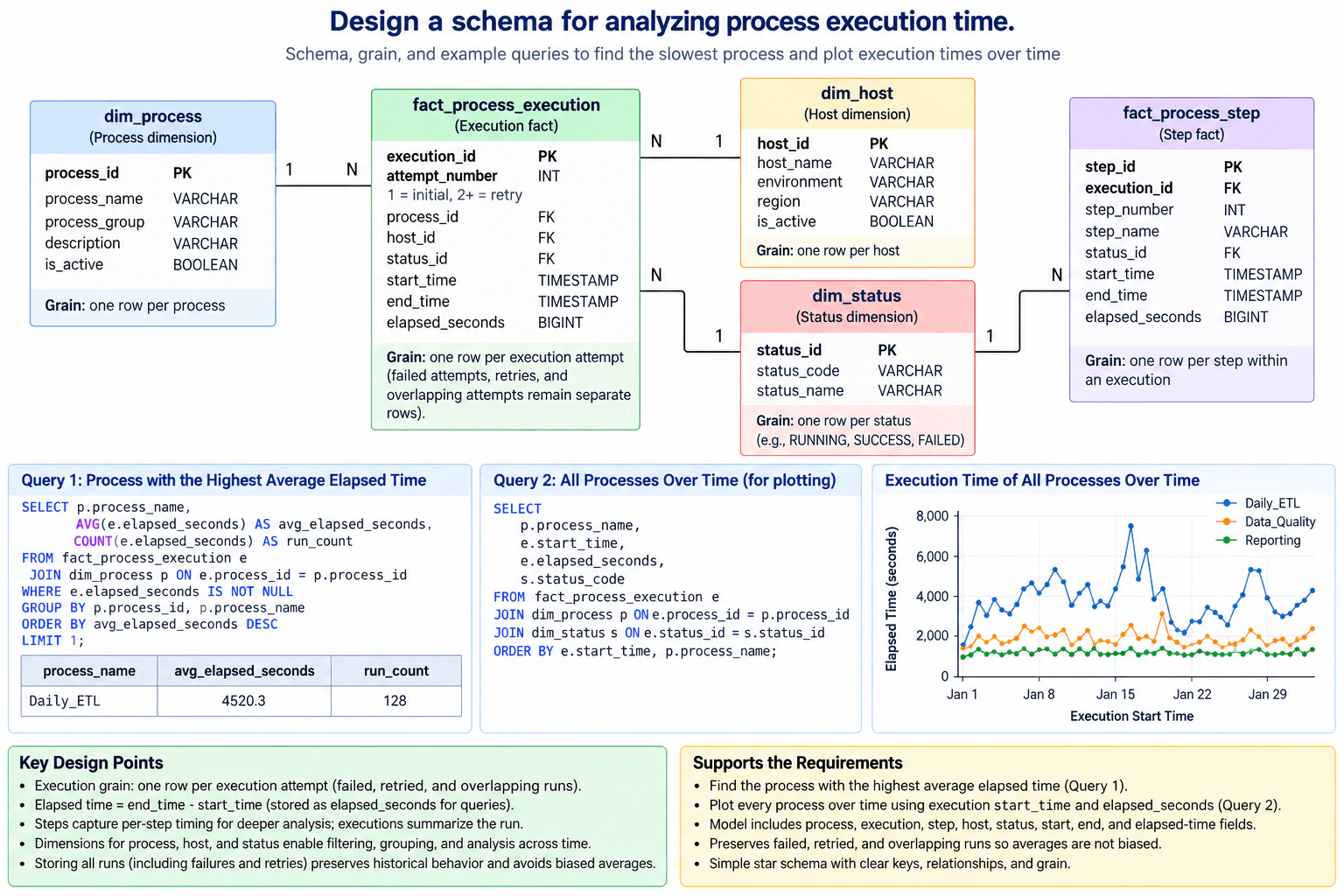
Create a model that lets a data scientist find the process with the highest average elapsed time and plot every process over time. Define process, execution, step, host, status, start, end, and elapsed-time fields; specify the execution grain; and preserve failed, retried, and overlapping runs so averages are not biased.

Short Interview Answer (30-60 seconds)

Use one fact row per execution attempt, linked to process, host, and status dimensions. Keep failed, retried, and overlapping attempts as separate rows. Store start, end, and elapsed time, and use a step fact for drill-down timing. Aggregate completed attempts by process and plot individual attempts over time.

Detailed Explanation

See the Code while reading this explanation.

The goal is to keep a complete history of every time a process runs. Each attempt gets its own record, even when it fails, is retried, or overlaps another attempt. The record stores when the attempt started, when it ended, and how long it took. Separate lists describe the process, machine, and result. Another table keeps the timing of individual steps inside an attempt. With this structure, a data scientist can compare average durations between processes and draw a timeline without replacing or losing important historical runs.

Useful Questions to Ask the Interviewer
  1. Should every retry count as a separate execution attempt when calculating average elapsed time?
  2. Should executions that are still running be excluded from the average until elapsed time is known?
  3. Is step-level timing needed only for drill-down analysis, or will step metrics be queried directly as well?
  4. Which time zone should be used consistently for execution and step timestamps?
Design a schema for analyzing process execution time. diagram
How to Explain It in an Interview

The central table is fact_process_execution. Its grain is one row per execution attempt. This is the most important modeling decision because an initial attempt, a failed attempt, a retry, and an overlapping attempt must remain separate historical events.

fact_process_execution uses execution_id as the primary key for each unique attempt. attempt_number records retry sequence: 1 is the initial attempt and 2 or greater is a retry. process_id, host_id, and status_id are foreign keys. start_time records when the attempt began, end_time records when it finished, and elapsed_seconds stores the duration used by analytical queries. For an unfinished attempt, end_time and elapsed_seconds may remain null until the attempt completes.

dim_process has one row per process. Its process_id primary key identifies fields such as process_name, process_group, description, and is_active. One process can have many execution attempts.

dim_host has one row per host. Its host_id primary key identifies host_name, environment, region, and is_active. One host can be associated with many execution attempts.

dim_status has one row per status. Its status_id primary key identifies status_code and status_name. The diagram uses statuses such as RUNNING, SUCCESS, and FAILED. One status can describe many execution attempts and many process-step rows.

fact_process_step stores step-level detail. Its grain is one row per step within an execution attempt. It contains step_id as the primary key, execution_id as a foreign key to the execution attempt, step_number, step_name, status_id as a foreign key to dim_status, start_time, end_time, and elapsed_seconds. This lets an analyst drill from a slow execution into the individual steps that consumed time.

To find the process with the highest average elapsed time, join fact_process_execution to dim_process, exclude rows whose elapsed_seconds is null, group by process_id and process_name, calculate AVG(elapsed_seconds), and sort the averages from highest to lowest. COUNT(elapsed_seconds) counts the same non-null execution attempts that contribute to the average. LIMIT 1 returns one process at the maximum position. If several processes tie for the same highest average, this form does not define which tied process must be returned unless an additional tie rule is added.

The diagram's teaching example shows Daily_ETL with an average elapsed time of 4520.3 seconds across 128 counted attempts. Those numbers are illustrative values from the approved diagram, not claims about a real production system.

For plotting execution time over time, keep the result at execution-attempt grain. Return process_name, start_time, elapsed_seconds, and status_code for each stored attempt. Join dim_process for the process label and dim_status for the execution status, then order by start_time and process_name. Failed attempts, retries, and overlapping attempts remain separate rows instead of being overwritten.

The main tradeoff is storage versus analytical correctness. Keeping every attempt increases row count, but it preserves history and avoids bias caused by retaining only successful or latest runs. The step fact adds more rows but enables detailed diagnosis of slow executions. The model should also use one documented time zone for timestamps. elapsed_seconds may be stored from end_time minus start_time, as shown in the diagram, but the ingestion process must keep those values consistent.

Key Insight / Why This Solution Works
  1. Declare fact_process_execution at one row per execution attempt.
  2. Store initial attempts, failed attempts, retries, and overlapping attempts as separate rows.
  3. Link each execution attempt to one process, host, and status.
  4. Store start_time, nullable end_time, and nullable elapsed_seconds on the execution fact.
  5. Store step-level timing in fact_process_step, linked by execution_id and status_id.
  6. For the average, filter to non-null elapsed_seconds, group by process, calculate AVG and the contributing count, then sort descending.
  7. For plotting, retain execution-attempt grain and return process, start time, elapsed time, and status for each attempt.
Code
-- PostgreSQL-compatible assumption because the question does not specify a dialect and the diagram uses LIMIT-style syntax.
-- Query 1: return one aggregated row for a process with the highest average completed elapsed time.
SELECT
  p.process_name,
  AVG(e.elapsed_seconds) AS avg_elapsed_seconds,
  COUNT(e.elapsed_seconds) AS run_count
FROM
  fact_process_execution AS e
  JOIN dim_process AS p ON e.process_id = p.process_id -- Each execution attempt belongs to one process.
WHERE
  e.elapsed_seconds IS NOT NULL -- Unfinished attempts do not contribute an unknown duration to AVG.
GROUP BY
  p.process_id,
  p.process_name -- Keep aggregation at unique process grain even if names are duplicated.
ORDER BY
  avg_elapsed_seconds DESC -- Highest average elapsed time appears first.
LIMIT
  1;


-- Returns one row; tied maxima need an explicit tie policy if all ties must be returned.
-- Query 2: keep one output row per execution attempt for time-series plotting.
SELECT
  p.process_name,
  e.start_time,
  e.elapsed_seconds,
  s.status_code
FROM
  fact_process_execution AS e
  JOIN dim_process AS p ON e.process_id = p.process_id -- Add the process label without changing execution-attempt grain.
  JOIN dim_status AS s ON e.status_id = s.status_id -- Add status such as RUNNING, SUCCESS, or FAILED.
ORDER BY
  e.start_time,
  p.process_name;


-- Sort chronologically, with process name as the secondary display order.
Why Interviewers Ask This

This question tests whether the candidate can choose the correct fact-table grain, separate descriptive entities from measurable events, model one-to-many relationships, preserve retries and failures without overwriting history, and write aggregation and time-series queries whose results remain analytically correct.

Common interview mistakes

Do not store only one mutable row per process, because that destroys execution history. Do not overwrite a failed attempt when a retry starts. Do not collapse overlapping attempts into one record. Do not average step rows when the required metric is execution duration, because processes with more steps would receive more weight. Do not use COUNT(*) beside AVG(elapsed_seconds) if the count is intended to represent only rows contributing to the average and elapsed_seconds can be null. Do not group only by process_name unless it is guaranteed unique. Also do not model RETRY as the lifecycle status when attempt_number already records retry sequence.

Interview tip

Lead with the grain: one row per execution attempt. Then explain why failures, retries, and overlaps stay separate. Walk through the process, host, status, and step relationships, and finish with the two consumer queries: aggregate completed attempts for the highest average and retain attempt-level rows for the time-series plot.

Interviewer may ask next
How would you handle an execution that is still running when the data scientist queries the model?

Keep the execution-attempt row because every attempt belongs in the history. Use a status such as RUNNING and leave end_time and elapsed_seconds null until the attempt finishes. The average query excludes null elapsed_seconds, so unfinished attempts do not distort the completed-attempt average. The plotting query can still retain the row when the consumer wants to show currently running attempts.

Why keep retries as separate rows instead of updating the failed execution?

A retry is a new execution attempt with its own execution_id, attempt_number, start time, end time, status, host, duration, and possibly different step behavior. Keeping it separate preserves the complete history and makes averages, failure analysis, and overlapping-run analysis reproducible. Updating the failed row would erase the original failed attempt and bias historical analysis.

3. Design a schema for cross-platform retention and conversion funnels.Data ModelingMediumMeta

Question Details

Represent exposures and ordered funnel actions across multiple application surfaces while preserving platform, session, privacy-safe user, campaign or experiment, and event time. Define conversion and cohort grains, attribution windows, repeated actions, identity-link confidence, and the data needed to compare retention without double counting one person across surfaces.

Short Interview Answer (30-60 seconds)

I would keep one row per event, map approved device or surface identities to a canonical person, derive one row per attributed conversion instance, and store retention at person-cohort-period grain. Repeated actions stay separate, attribution uses a defined lookback window, and retention counts distinct people.

Detailed Explanation

The goal is to record what a person sees and does across web, mobile, TV, or other application surfaces, then compare how many people move through a sequence and return later. The design must keep each action separate, remember when and where it happened, connect the same person across surfaces only when that connection is trusted, and keep marketing or experiment information. It also needs clear rules for which earlier exposure gets credit for a later conversion and for counting a returning person only once even if that person used several surfaces.

Useful Questions to Ask the Interviewer
  1. What event defines the start of a cohort: first conversion, signup, or another qualifying action?
  2. What ordered actions define each funnel, and can the same action happen more than once?
  3. What attribution rule and lookback window should apply, such as the most recent qualifying exposure within 7 or 28 days?
  4. What identity-link confidence threshold and link methods are approved for cross-surface person-level reporting?
  5. What activity qualifies a person as retained in each cohort period?
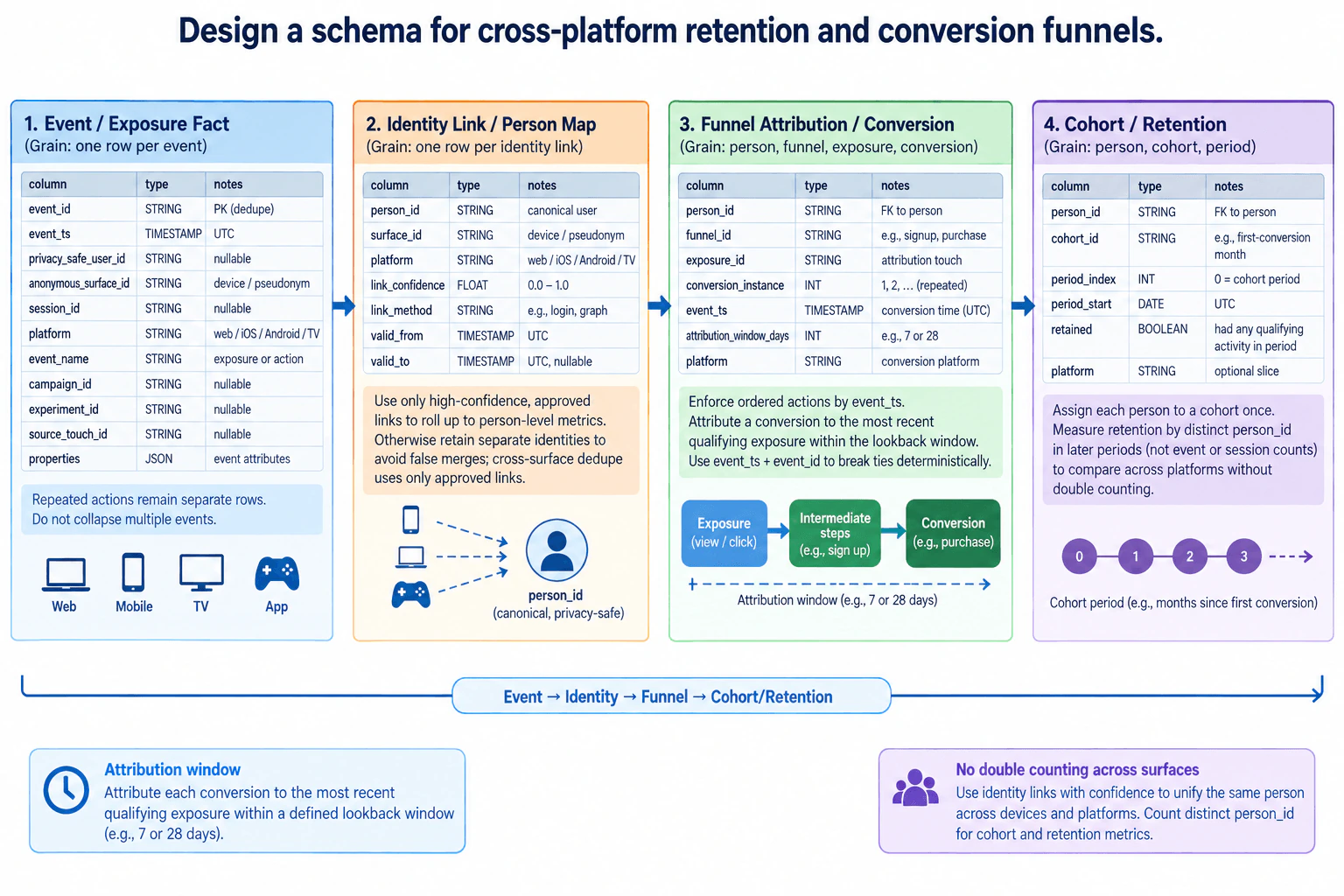
Design a schema for cross-platform retention and conversion funnels. diagram
How to Explain It in an Interview

Start with the grains because they determine whether later metrics are correct.

No SQL dialect is specified, and this is a conceptual data-modeling question, so executable SQL is not necessary.

The Event / Exposure Fact has grain one row per event. event_id is the primary event key and supports deduplication. The row keeps event_ts in UTC, nullable privacy_safe_user_id, anonymous_surface_id for a device or pseudonymous surface identity, nullable session_id, platform, event_name, nullable campaign_id, nullable experiment_id, nullable source_touch_id, and event properties. Exposures and funnel actions stay at this event grain. Repeated actions remain separate rows rather than being collapsed.

The Identity Link / Person Map has grain one row per identity link. person_id is the canonical privacy-safe person used for cross-platform analysis. surface_id represents the device or pseudonymous identity that is linked to that person, platform identifies the application surface, link_confidence records how strong the match is, link_method records how the link was established, and valid_from plus nullable valid_to define when that mapping is valid. Event-side identities such as anonymous_surface_id are resolved through this map. Only approved high-confidence links roll identities into person-level metrics. Unapproved or uncertain identities stay separate to avoid false merges; cross-surface deduplication uses only approved links.

Next, derive Funnel Attribution / Conversion at grain person, funnel, exposure, conversion. Keep person_id, funnel_id, exposure_id, conversion_instance, event_ts, attribution_window_days, and the conversion platform. Funnel actions are ordered by event_ts. If two events have the same timestamp, event_id is the deterministic tie breaker. conversion_instance lets repeated conversions by the same person remain distinct instead of overwriting one another.

For attribution, apply one explicit rule consistently. The diagram uses the most recent qualifying exposure within a defined lookback window, for example 7 or 28 days. A conversion can therefore receive credit only from an exposure that happened before it and falls inside that window. exposure_id identifies the selected attribution touch. Campaign and experiment context remains available from the underlying event data for analysis.

Finally, build Cohort / Retention at grain person, cohort, period. Store person_id, cohort_id, period_index, period_start, retained, and an optional platform slice. In this design the example cohort anchor is first conversion, such as first-conversion month. period_index 0 is the cohort period, and later indexes represent later cohort periods. retained is true when the person has qualifying activity in that period.

The key rule for cross-platform retention is to count distinct person_id values after approved identity resolution, not events, sessions, devices, or surface identifiers. A person who returns through both web and mobile in the same period is therefore one retained person, not two. Platform can still be kept as a reporting slice, but an overall person-level retention metric must not be produced by simply summing overlapping platform counts.

The main tradeoff is identity quality. A strict confidence threshold reduces false merges but can leave the same real person represented by separate identities. A loose threshold increases apparent cross-surface coverage but risks incorrectly merging different people. Keeping link confidence, link method, and validity boundaries makes the policy explicit and auditable.

Technical Approach
  1. Ingest every exposure and funnel action as a separate event row keyed by event_id and timestamped in UTC.
  2. Resolve device or pseudonymous surface identities to person_id only through approved identity links, using link confidence and validity boundaries.
  3. For each person and funnel, order actions by event_ts and event_id while preserving repeated occurrences.
  4. Number repeated conversions with conversion_instance.
  5. For each conversion, select the most recent qualifying prior exposure inside the configured attribution window and store that exposure_id.
  6. Assign each person once to the chosen cohort, such as first-conversion month.
  7. For every cohort period, mark whether that person had qualifying activity.
  8. Compute cross-platform retention from distinct person_id values, using platform only as an optional slice rather than summing overlapping platform counts.
Practical Insights

Storage grows with the number of raw events because repeated actions are intentionally retained. Identity mapping adds history proportional to linked surface identities and mapping changes. Funnel processing requires events for a person to be grouped and ordered, so large histories can require significant sorting or partitioned processing. Attribution adds a bounded time-based lookup from each conversion to earlier exposures. Retention becomes cheaper after person-cohort-period rows are materialized because reporting works from the already-defined analytical grain. Maintenance cost mainly comes from keeping funnel definitions, attribution windows, identity policies, cohort rules, and qualifying-retention activity consistent over time.

Why Interviewers Ask This

This tests whether the candidate can choose correct analytical grains, preserve event history, model identity safely across application surfaces, handle repeated funnel actions, define deterministic attribution, and compute retention without cross-platform double counting. It also tests judgment around uncertain identity links, cohort definitions, timestamps, campaign or experiment attribution, and the boundary between raw events and derived analytical facts.

Common interview mistakes

Common mistakes are counting sessions or devices instead of people for cross-platform retention; merging low-confidence identities and creating false person matches; dropping anonymous events that may later become linkable; collapsing repeated funnel actions into one record; ignoring event order or timestamp ties; attributing a conversion to an exposure outside the lookback window; failing to require the exposure to precede the conversion; assigning the same person multiple times to the same cohort; summing per-platform retained-user counts even though one person can appear on several platforms; and changing identity mappings without effective-time boundaries.

Interview tip

Lead with the four grains: event, identity link, attributed conversion, and person-cohort-period. Then explain the two correctness rules: attribution uses an explicit ordered lookback rule, and cross-platform retention counts distinct canonical people only after approved identity resolution.

Interviewer may ask next
How would you handle a person who converts multiple times after several exposures?

Keep every conversion as a separate conversion instance rather than collapsing them. For each conversion, independently select the most recent qualifying exposure that occurred before it and within the configured attribution window. The same person can therefore have conversion_instance 1, 2, and later values, each preserving its own attributed exposure_id.

What should happen when identity-link confidence is too low to safely merge two surface identities?

Do not merge them into the same person_id for cross-platform metrics. Keep the identities separate until an approved link satisfies the required policy. Store the confidence, linking method, and validity interval so the decision remains auditable. This avoids false merges, although the tradeoff is that one real person may temporarily remain represented by multiple identities and cannot be perfectly de-duplicated until stronger evidence exists.

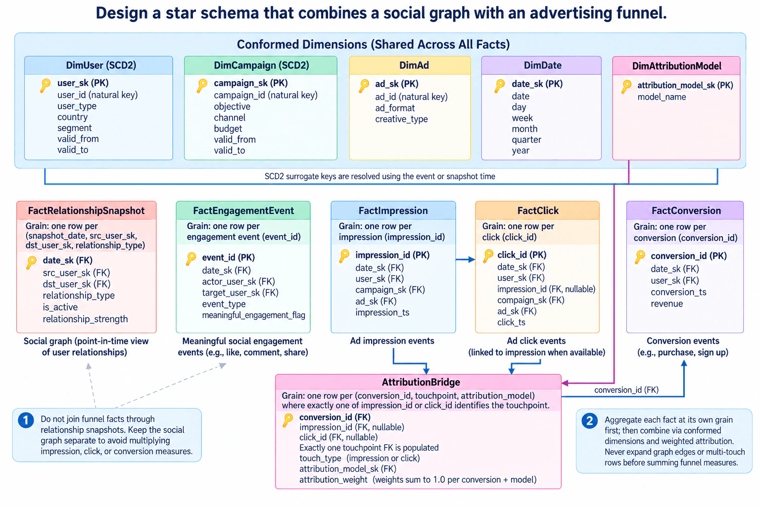
4. Design a star schema that combines a social graph with an advertising funnel.Data ModelingHardMeta

Question Details

Model meaningful engagement and the path from ad impression through click and conversion while social relationships and campaign attributes change. Declare the grains of relationship snapshots, engagement events, impressions, clicks, and conversions; define conformed dimensions and attribution records; and prevent graph expansion or multi-touch joins from multiplying funnel measures.

Short Interview Answer (30-60 seconds)

I would use separate facts for relationship snapshots, engagement, impressions, clicks, and conversions, with conformed dimensions. Historical user and campaign keys are resolved by event time. Multi-touch attribution lives in a bridge, and each fact is aggregated at its own grain before results are combined.

Detailed Explanation

The goal is to organize two kinds of information together without accidentally counting the same activity more than once. One side records how people are connected and how those connections change over time. The other records the path from seeing an advertisement to clicking it and finally completing an action. The design must also remember what users and campaigns looked like when each activity happened. When one completed action can receive credit from several earlier interactions, that credit is stored separately so the original impression, click, conversion, and revenue totals stay correct.

Useful Questions to Ask the Interviewer
  1. Which relationship types should the social graph snapshot contain, such as follow, friend, or connect?
  2. Which engagement event types count as meaningful engagement?
  3. Should conversions support impression touchpoints, click touchpoints, or both?
  4. Which attribution models are required, and should attribution weights sum to 1.0 for each conversion and model?
  5. How frequently should relationship snapshots be captured?
Design a star schema that combines a social graph with an advertising funnel. diagram
How to Explain It in an Interview

I would start by declaring the grain of every fact table. Different business processes have different natural grains, so I would not force them into one wide fact table.

FactRelationshipSnapshot has one row per snapshot_date, src_user_sk, dst_user_sk, and relationship_type. It contains date_sk, src_user_sk, dst_user_sk, relationship_type, is_active, and relationship_strength. Both src_user_sk and dst_user_sk are role-playing references to the same conformed DimUser. This table gives a point-in-time view of the social graph.

FactEngagementEvent has one row per engagement event identified by event_id. It contains date_sk, actor_user_sk, target_user_sk, event_type, and meaningful_engagement_flag. actor_user_sk and target_user_sk also reference DimUser in different roles. This keeps meaningful social engagement separate from advertising events.

FactImpression has one row per impression_id. It contains date_sk, user_sk, campaign_sk, ad_sk, and impression_ts. FactClick has one row per click_id and contains date_sk, user_sk, nullable impression_id, campaign_sk, ad_sk, and click_ts. The nullable impression_id links a click to its originating impression when that relationship is known.

FactConversion has one row per conversion_id. It contains date_sk, user_sk, conversion_ts, and revenue. It deliberately does not contain one campaign_sk or ad_sk, because a conversion may receive credit from multiple advertising touchpoints.

The conformed dimensions are DimUser, DimCampaign, DimAd, DimDate, and DimAttributionModel. A conformed dimension is a shared dimension whose keys and meaning are reused consistently by the fact tables that need it. DimUser uses user_sk as its surrogate primary key and user_id as its natural key. It is SCD2, so historical versions carry valid_from and valid_to. DimCampaign is also SCD2 and contains campaign_sk, campaign_id, objective, channel, budget, valid_from, and valid_to. DimAd contains ad_sk, ad_id, ad_format, and creative_type. DimDate contains date_sk plus date, day, week, month, quarter, and year. DimAttributionModel contains attribution_model_sk and model_name.

For SCD2 dimensions, the surrogate-key lookup uses the event or snapshot time. An old impression, click, engagement event, or relationship snapshot therefore keeps pointing to the user or campaign version that was valid when that activity happened rather than to the current version.

Multi-touch credit belongs in AttributionBridge. Its grain is one row per conversion_id, touchpoint, and attribution model. It stores conversion_id, nullable impression_id, nullable click_id, touch_type, attribution_model_sk, and attribution_weight. Exactly one of impression_id or click_id is populated for a bridge row, so the touchpoint is unambiguous. attribution_model_sk references DimAttributionModel. For each conversion and attribution model, the attribution weights sum to 1.0.

The most important correctness rule is to aggregate each fact at its own grain before combining results. Count impressions from FactImpression, clicks from FactClick, and conversions or revenue from FactConversion. Do not directly join raw relationship edges, impressions, clicks, conversions, and multi-touch attribution rows into one expanded row set, because one-to-many and many-to-many joins can multiply the same funnel measures.

For attributed revenue, start with one conversion, join its AttributionBridge rows by conversion_id, follow the single populated touchpoint key to either FactImpression or FactClick, and use that touchpoint's campaign or ad context. Multiply the conversion revenue by attribution_weight, then aggregate the weighted values by the desired conformed dimension and attribution model. This keeps the original conversion revenue intact for each attribution model while still supporting multiple credited touchpoints.

The main tradeoff is that this design uses several fact tables rather than one large funnel table. Queries require more deliberate aggregation, but the model preserves natural grain, historical context, role-playing user relationships, and multi-touch attribution while avoiding fan-out errors.

Key Insight / Why This Solution Works
  1. Declare the grain of each fact table.
  2. Store social relationships as point-in-time relationship snapshots.
  3. Store meaningful engagement, impressions, clicks, and conversions as separate event facts.
  4. Reuse conformed user, campaign, ad, date, and attribution-model dimensions where applicable.
  5. Resolve SCD2 user and campaign surrogate keys using event or snapshot time.
  6. Link a click to an impression with nullable impression_id when known.
  7. Keep FactConversion independent of a single campaign or ad.
  8. Store conversion-to-touchpoint credit in AttributionBridge with exactly one impression or click touchpoint per row.
  9. Make attribution weights sum to 1.0 per conversion and attribution model.
  10. Aggregate each fact at its declared grain before combining results through conformed dimensions or weighted attribution.
Why Interviewers Ask This

This tests whether the candidate can declare fact-table grain correctly, model changing user and campaign attributes, use conformed dimensions and SCD2 history, represent multi-touch attribution, and prevent graph expansion or many-to-many attribution joins from multiplying funnel measures.

Common interview mistakes

Common mistakes are combining relationships, engagement, impressions, clicks, and conversions into one fact table even though they have different grains; expanding graph neighbors before calculating funnel metrics; joining raw impression, click, conversion, and attribution rows before aggregation; storing one campaign or ad on FactConversion even though multiple touchpoints may receive credit; populating both impression_id and click_id in one AttributionBridge row; failing to make attribution weights sum to 1.0 per conversion and attribution model; joining DimAttributionModel directly to FactConversion instead of through AttributionBridge; and resolving an SCD2 user or campaign to its current version instead of the version valid at the event or snapshot time.

Interview tip

Lead with the five fact grains. Then explain the conformed dimensions, role-playing user keys, SCD2 time lookup, and AttributionBridge. Finish with the correctness rule: aggregate each fact at its own grain before combining results, and never expand graph edges or multi-touch rows before summing funnel measures.

Interviewer may ask next
How would you calculate attributed campaign revenue without double counting conversions?

Start from FactConversion at one row per conversion and join to AttributionBridge by conversion_id. For each bridge row, exactly one touchpoint key is populated. Follow impression_id to FactImpression or click_id to FactClick, obtain that touchpoint's campaign context, multiply conversion revenue by attribution_weight, and then aggregate by campaign_sk and attribution_model_sk. Because the weights sum to 1.0 for each conversion and attribution model, the weighted campaign amounts preserve the original conversion revenue total for that model.

How would you handle a campaign or user attribute that changes after an event occurred?

Resolve the SCD2 surrogate key that was valid at the event or snapshot time. DimUser and DimCampaign keep historical rows using valid_from and valid_to boundaries. During ingestion, the fact looks up the dimension version whose validity interval contains its timestamp and stores that surrogate key. The fact therefore continues to reference the historically correct dimension version even after the natural-key entity changes.

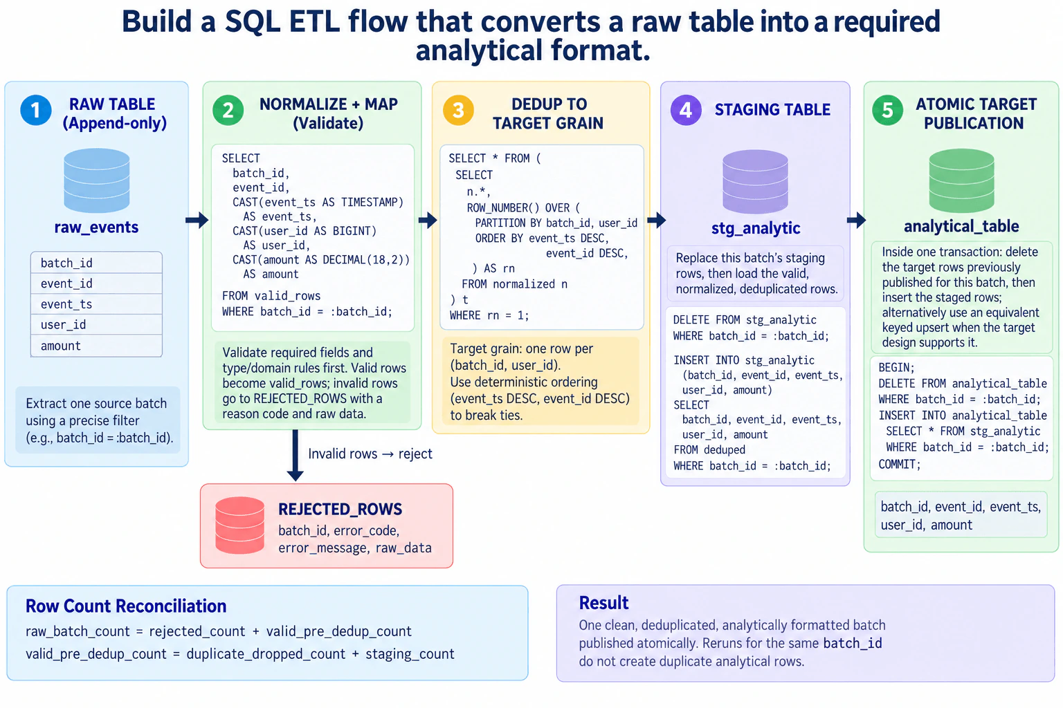
5. Build a SQL ETL flow that converts a raw table into a required analytical format.Data PipelinesEasyMeta

Question Details

Start with an append-only raw table and a precisely defined target grain. Design the extraction filter, type normalization, field mapping, deduplication, rejected-row path, staging table, and atomic target publication. State how a rerun for the same source batch avoids duplicate rows and how row counts reconcile from raw input to the desired output.

Short Interview Answer (30-60 seconds)

I would process one batch_id at a time, validate rows before casting them, quarantine invalid rows, normalize the valid rows, and deduplicate to one row per (batch_id, user_id) using deterministic ordering. I would replace that batch in staging, then delete and insert its target rows inside one transaction. That makes same-batch reruns idempotent. I would also reconcile raw, rejected, duplicate-dropped, and staged counts. The trade-off is extra staging and write work in exchange for simpler recovery and stronger correctness.

Detailed Explanation

See the Code while reading this explanation.

The goal is to take one group of newly received records and turn it into a clean set of rows that can be used for analysis. Some input records may be incomplete, badly formed, or repeated. Those records must not silently disappear. Bad records are kept separately with an explanation, repeated records are reduced in a predictable way, and good records are prepared before they become visible in the final result. If the same group is processed again, the result should stay the same instead of creating extra copies.

Useful Questions to Ask the Interviewer
  1. Is (batch_id, user_id) the exact required target grain?
  2. Which required-field, type, and domain rules define whether a row is valid?
  3. Should event_ts DESC, event_id DESC be the required deterministic winner when duplicate rows exist?
  4. Does the target table retain batch_id so one source batch can be safely replaced?
Build a SQL ETL flow that converts a raw table into a required analytical format. diagram
How to Explain It in an Interview
1. Extract one append-only source batch

I would start by isolating exactly one source batch from raw_events. The visible source contract contains batch_id, event_id, event_ts, user_id, and amount. The extraction filter is WHERE batch_id = :batch_id. This gives the run a clear identity and prevents one execution from mixing unrelated batches. Because the source is append-only, I do not modify the original source records. The selected rows then move to validation and normalization.

2. Validate before normalizing and mapping

I would validate required fields plus the type and domain rules before doing conversions that could fail. Valid records become valid_rows. Invalid records go to REJECTED_ROWS with batch_id, error_code, error_message, and raw_data. That keeps failures visible instead of silently dropping them. Only valid_rows move through the successful path. Their values are mapped to the analytical contract: event_ts becomes a timestamp, user_id becomes a big integer, and amount becomes DECIMAL(18,2).

3. Deduplicate to the exact target grain

Next I would enforce one row per (batch_id, user_id). I would calculate ROW_NUMBER() inside each (batch_id, user_id) group and order by event_ts DESC, event_id DESC. The row with rn = 1 wins. Using event_id as the second ordering field makes the choice deterministic when two rows have the same event time. That is important for reruns because the same input batch should produce the same deduplicated output.

4. Replace the batch in staging

The deduplicated rows move into stg_analytic. Before inserting them, I delete any existing staging rows for the same batch_id. I then insert the newly deduplicated rows. This makes the staging operation safe to repeat: rerunning one batch replaces that batch's staged rows instead of accumulating another copy. The staging table also creates a clear boundary between transformation work and final target publication.

5. Publish atomically to the analytical table

For analytical_table, I use one database transaction. Inside that transaction, I delete rows already published for the same batch_id, insert that batch from stg_analytic, and then commit. A same-batch rerun therefore replaces the previous analytical result rather than appending duplicates. The transaction is the publication boundary: the delete and insert belong to one unit of work. An equivalent keyed upsert could be used when the target design supports it, but the audited design uses transactional delete-and-insert.

6. Reconcile the row counts

Finally, I verify the batch with two equations. First, raw_batch_count = rejected_count + valid_pre_dedup_count. Second, valid_pre_dedup_count = duplicate_dropped_count + staging_count. Together, they account for every raw record across validation and deduplication. This is important because a completed SQL task does not by itself prove that the data is correct. If either equation fails, I would not consider the batch successfully reconciled even if the target transaction completed.

Technical Approach

1. Filter raw_events to the requested batch_id. 2. Validate required fields plus type and domain rules; route invalid records to REJECTED_ROWS. 3. Cast and map only valid_rows into the target types. 4. Deduplicate with ROW_NUMBER() partitioned by (batch_id, user_id) and ordered by event_ts DESC, event_id DESC; keep rn = 1. 5. Delete the same batch from stg_analytic and insert the new deduplicated rows. 6. In one transaction, delete that batch_id from analytical_table, insert it from staging, and commit. 7. Reconcile raw, rejected, duplicate-dropped, and staged counts.

Practical Insights

The main cost is reading, validating, sorting, and writing one batch. Validation and mapping grow roughly with the number of input rows. Deduplication is usually the most expensive step because rows must be grouped by (batch_id, user_id) and ordered by event_ts and event_id. The benefit is deterministic output and simple rerun behavior. The downside is extra staging storage plus delete-and-insert work for each batch. The final transaction may also hold database resources while publication runs. We accept this because the result is easier to reason about and recover. Row-count reconciliation adds a little work, but it gives strong evidence that rows were not silently lost or duplicated.

Code
-- Step 1: read exactly one append-only source batch.
SELECT
  batch_id,
  event_id,
  event_ts,
  user_id,
  amount
FROM
  raw_events
WHERE
  batch_id = ?;


-- Step 2: validation happens before this successful path.
-- Invalid records are written to REJECTED_ROWS with batch_id,
-- error_code, error_message, and raw_data.
-- Only validated records enter valid_rows and are normalized here.
SELECT
  batch_id,
  event_id,
  CAST(event_ts AS TIMESTAMP) AS event_ts,
  CAST(user_id AS BIGINT) AS user_id,
  CAST(amount AS DECIMAL(18, 2)) AS amount
FROM
  valid_rows
WHERE
  batch_id = ?;


-- Step 3: enforce one deterministic row per (batch_id, user_id).
SELECT
  *
FROM
  (
    SELECT
      n.*,
      ROW_NUMBER() OVER (
        PARTITION BY
          batch_id,
          user_id
        ORDER BY
          event_ts DESC,
          event_id DESC
      ) AS rn
    FROM
      normalized n
  ) t
WHERE
  rn = 1;


-- Step 4: replace this batch in staging so reruns do not accumulate copies.
DELETE FROM stg_analytic
WHERE
  batch_id = ?;


INSERT INTO
  stg_analytic (batch_id, event_id, event_ts, user_id, amount)
SELECT
  batch_id,
  event_id,
  event_ts,
  user_id,
  amount
FROM
  deduped
WHERE
  batch_id = ?;


-- Step 5: publish the same batch as one target transaction.
-- The delete and insert form the atomic publication boundary.
BEGIN;


DELETE FROM analytical_table
WHERE
  batch_id = ?;


INSERT INTO
  analytical_table (batch_id, event_id, event_ts, user_id, amount)
SELECT
  batch_id,
  event_id,
  event_ts,
  user_id,
  amount
FROM
  stg_analytic
WHERE
  batch_id = ?;


COMMIT;


-- Step 6: reconcile every source row across validation and deduplication.
-- raw_batch_count = rejected_count + valid_pre_dedup_count
-- valid_pre_dedup_count = duplicate_dropped_count + staging_count
Why Interviewers Ask This

This question tests whether a candidate can turn a simple transformation request into a reliable batch pipeline. The interviewer is looking for judgment around source and target grain, validation, deterministic deduplication, rejected records, staging, transaction boundaries, idempotent reruns, and reconciliation. A strong answer shows that successful SQL execution alone is not enough: the candidate must also prove that rows were neither silently lost nor duplicated and that repeated processing produces the same business result.

Common interview mistakes

Common mistakes are appending directly to the target on every rerun, deduplicating without a deterministic tie-breaker, converting malformed raw values before validation, dropping bad records without recording why they were rejected, and treating successful SQL execution as proof that the data is correct. Another mistake is changing the grain accidentally, such as deduplicating only by user_id while the audited design uses (batch_id, user_id). Publishing the target delete and insert as separate committed operations can expose an incomplete replacement. Finally, checking only the final row count is not enough; rejected and duplicate-dropped counts must reconcile with the raw input.

Interview tip

Explain the design in the same order as the data moves: batch filter, validation, normalization, deterministic deduplication, staging replacement, atomic target publication, and reconciliation. Emphasize two correctness ideas: the target grain is explicit and same-batch reruns are idempotent. Finish with the two reconciliation equations. That shows you are thinking about business-result correctness, not just whether the SQL statements completed.

Interviewer may ask next
What would you do if processing the same batch fails and must be rerun?

I would keep the same architecture and rerun the same batch_id. The requirement that changes is recovery, not the data contract. The staging step is already safe to repeat because it deletes that batch from stg_analytic before loading the newly deduplicated rows. The final target publication is also repeatable because it deletes the same batch_id and reinserts that batch inside one transaction. Validation and deduplication do not change, so the rerun uses the same rules and produces the same deterministic winners. After the rerun, I would execute the same reconciliation checks again: raw equals rejected plus valid-before-dedup, and valid-before-dedup equals duplicates-dropped plus staging. If either check fails, I would not treat recovery as complete. The main downside is repeated read, sort, and write work for that batch, but the benefit is simple recovery without adding a separate replay architecture or allowing duplicate analytical rows.

What if two duplicate records have exactly the same event timestamp?

I would keep the existing deterministic secondary ordering on event_id. The target grain remains one row per (batch_id, user_id), but event_ts alone is no longer enough to choose one winner when two records tie. The affected component is the ROW_NUMBER() expression. It orders by event_ts DESC, event_id DESC, so event_id breaks the tie and the same source batch produces the same selected row on every rerun. The validation path, REJECTED_ROWS, staging replacement, final transaction, and reconciliation all remain unchanged. If the interviewer says event_id is not a valid business tie-breaker, I would ask which deterministic field should be used instead rather than inventing one. The downside of using additional ordering columns is slightly more sorting work, but deterministic output is more important because reliable idempotent reruns depend on choosing the same duplicate winner each time.

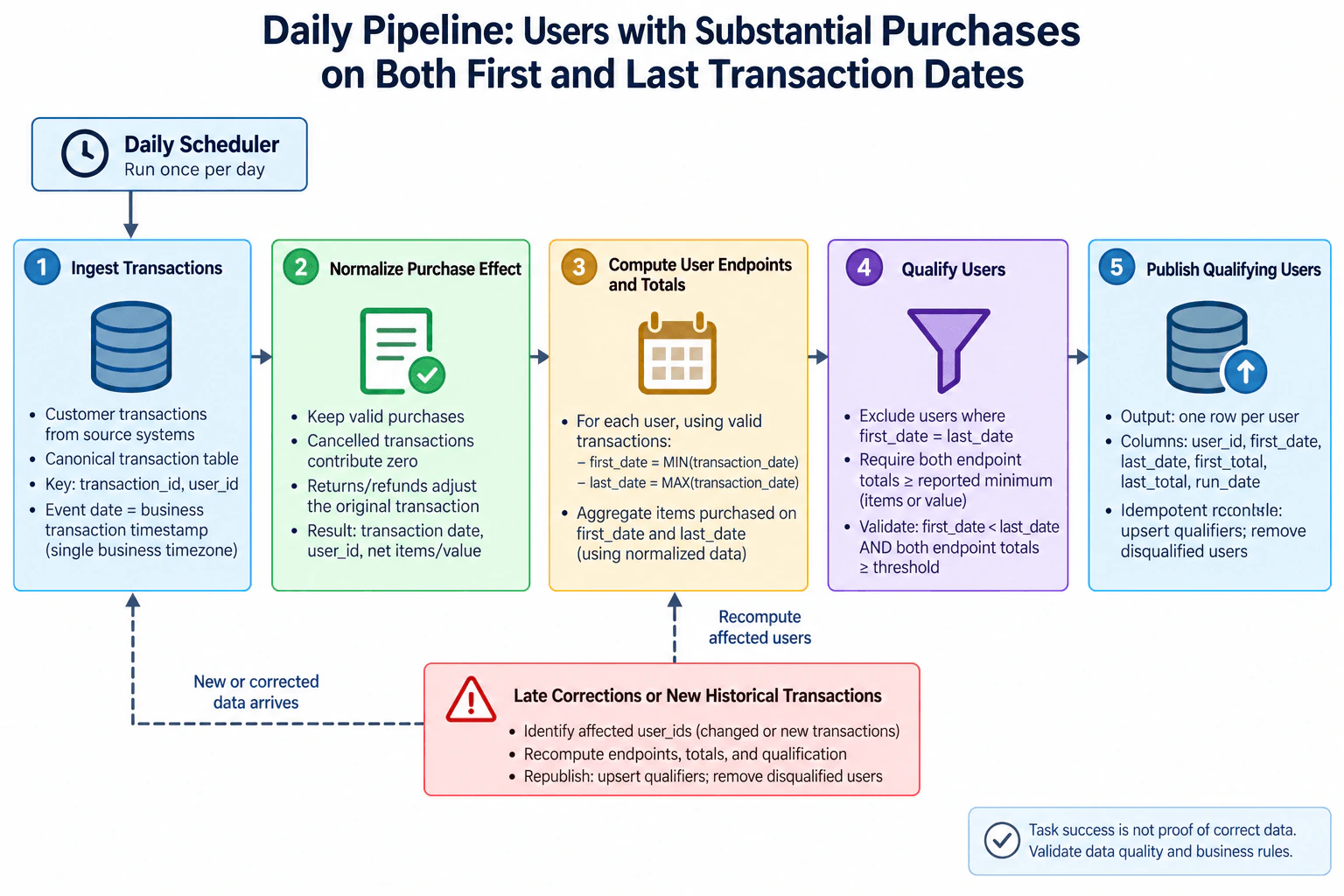
6. Build a daily pipeline that identifies users with substantial purchases on both their first and last transaction dates.NEWData PipelinesEasyMeta

Question Details

Ingest customer transactions, establish each user’s first and last transaction dates, aggregate items purchased on those dates, and publish users meeting the reported minimum on both endpoints while excluding single-transaction users. Define transaction identity, date boundaries, cancellations and returns, late corrections, incremental recomputation, and an idempotent output grain of one qualifying user.

Short Interview Answer (30-60 seconds)

I would build a daily batch pipeline that ingests customer transactions, normalizes cancellations and returns, finds each user's first and last valid transaction dates, and totals purchases on those dates. I would exclude users whose first and last valid dates are the same and require both endpoint totals to meet the reported minimum. The output is one current row per qualifying user. Late corrections recompute only affected users, and publication reconciles both newly qualifying and newly disqualified users. The trade-off is simple daily processing versus fresher results.

Detailed Explanation

The goal is to create a daily list of customers who bought enough on both their earliest valid purchase day and their latest valid purchase day. First, collect the purchase records and remove the effect of cancelled activity while applying returns to the purchase they belong to. Then find the earliest and latest valid dates for each customer and total what was bought on those two dates. Customers whose earliest and latest valid dates are the same are excluded. If older information changes, recalculate only the affected customers and update the published list so it reflects who currently qualifies.

Useful Questions to Ask the Interviewer
  1. What exactly defines one transaction, and is transaction_id unique within a user or globally?
  2. Which business timezone defines transaction_date?
  3. Is the reported minimum based on item quantity, monetary value, or another supplied measure?
  4. Should a return or refund always adjust its original transaction rather than count on the return date?
  5. How far back can corrections arrive, and should the destination represent the current qualifying set or historical daily snapshots?
Build a daily pipeline that identifies users with substantial purchases on both their first and last transaction dates. diagram
How to Explain It in an Interview
1. Ingest Transactions

I would start with the transaction contract shown in the design. The source is customer transactions from source systems, represented in a canonical transaction table. Each record has a stable transaction_id, a user_id, and a business transaction timestamp. I derive transaction_date from that timestamp using the agreed business timezone. The Daily Scheduler starts this pipeline once per day, and Stage 1 feeds Stage 2 before any downstream computation begins.

2. Normalize Purchase Effect

Next, I would normalize the business effect of each transaction. Valid purchases contribute their items or value. Cancelled transactions contribute zero and are not treated as valid endpoint transactions. Returns and refunds adjust the original transaction rather than creating a new purchase endpoint on the return date. The normalized data passed forward contains the transaction date, user identifier, and normalized items or value needed for endpoint calculations.

3. Compute User Endpoints and Totals

For each user, using valid transactions, I calculate first_date as the minimum transaction_date and last_date as the maximum transaction_date. I then aggregate the normalized items or value from all valid transactions occurring on those two dates. This matters because a user may have several purchases on the same endpoint date. The result at this stage is one user with a first date, last date, first endpoint total, and last endpoint total.

4. Qualify Users

I next apply the business rules shown in the diagram. Users where first_date equals last_date are excluded, which is how this design removes users without two distinct valid transaction dates. For everyone else, both the first endpoint total and last endpoint total must meet the reported minimum. The pipeline uses the exact supplied definition of that minimum, whether it is based on items, value, or another approved measure. I also validate that first_date is earlier than last_date and that both endpoint totals satisfy the threshold before publication.

5. Publish Qualifying Users

The destination grain is one current row per qualifying user_id. The published record contains the user identifier, first date, last date, first total, last total, and run date. Publication is an idempotent reconciliation rather than an insert-only operation. Qualifying users are inserted or updated, while users who were previously published but no longer qualify are removed. This prevents stale qualifying rows after historical corrections.

6. Handle Late Corrections and Verify the Result

When a new historical transaction or a correction arrives, I identify the affected user_id values. Those users re-enter at the endpoint computation stage, where I recompute their valid first and last dates, endpoint totals, and qualification. They then follow the same Stage 3 to Stage 4 to Stage 5 flow as the normal pipeline. Recomputing only affected users reduces unnecessary work while preserving the same business rules. Finally, I do not treat task success as proof of correct data. I validate the endpoint dates, threshold conditions, and published current-user set before considering the result correct.

Technical Approach
  1. Run the pipeline once per day with the Daily Scheduler.
  2. Ingest customer transactions into the canonical transaction input used by the pipeline.
  3. Use stable transaction_id and user_id values and derive transaction_date from the business transaction timestamp in the agreed timezone.
  4. Normalize purchase effects: keep valid purchases, make cancelled transactions contribute zero, and apply returns or refunds to the original transaction.
  5. For each user, use valid transactions to calculate first_date = MIN(transaction_date) and last_date = MAX(transaction_date).
  6. Aggregate normalized items or value across all transactions on first_date and last_date.
  7. Exclude users where first_date = last_date.
  8. Keep only users whose first and last endpoint totals both meet the reported minimum.
  9. Reconcile the destination at one current row per qualifying user: upsert current qualifiers and remove users who have become disqualified.
  10. When late or corrected historical data arrives, identify affected users and rerun endpoint computation, qualification, and reconciliation for those users.
  11. Validate the endpoint and qualification rules independently of scheduler or task success.
Practical Insights

The benefit is that a daily batch pipeline is simple to understand and operate, and it matches the requested daily result. For N transaction records, the main cost comes from reading, grouping, and aggregating the relevant transaction history. Incremental recomputation reduces that cost when a late correction affects only a small number of users. The downside is that a current result needs reconciliation, not just inserts, because a correction can make an existing user stop qualifying. Strong validation may add some processing time, but we accept this because successful tasks do not prove the business result is correct. Daily scheduling also trades freshness for simplicity: changes may wait until the next run instead of appearing immediately.

Why Interviewers Ask This

This question tests whether a candidate can turn a business rule into a correct daily data product. The interviewer is looking for judgment around transaction identity, date boundaries, endpoint aggregation, cancellations and returns, late corrections, incremental recomputation, and idempotent publication. It also tests whether the candidate understands that a successful scheduled task does not prove the business data is correct and that historical changes can alter both endpoint dates and user qualification.

Common interview mistakes

Common mistakes are finding first and last dates before handling cancellations, letting a cancelled transaction define an endpoint, treating a later return date as a new purchase date instead of adjusting the original transaction, and counting only one transaction when multiple purchases occurred on the same endpoint date. Another mistake is publishing with upserts only: a user who becomes disqualified after a correction would remain as stale output. Candidates also forget to rerun qualification after endpoint recomputation, recompute every user when only a small affected set changed, or assume that a successful scheduled task proves the published data is correct.

Interview tip

Start with the grain: customer transactions go in and one current qualifying row per user comes out. Then walk through the five stages in order: ingest, normalize, compute endpoints, qualify, and reconcile publication. Spend extra time on late corrections and removing users who stop qualifying, because those details show that you understand business correctness rather than only the happy-path batch job.

Interviewer may ask next
What would you change if late historical corrections became frequent and recomputing every user's full history each day became too expensive?

I would keep the same business rules and destination contract but make the correction path more targeted. The requirement that changes is processing cost, not qualification logic. During ingestion, I would identify the user_id values touched by new or corrected historical transactions. Only those users would re-enter Stage 3. For each affected user, I would recompute the first and last valid transaction dates and the totals on those dates, then run the same qualification rule and Stage 5 reconciliation.

I would not patch only the changed total. A historical record can become a new first date, stop being the first date, change the last date, or change an endpoint total. Recomputing the affected user's endpoints from valid history preserves correctness. Publication still upserts current qualifiers and removes users who become disqualified. The same endpoint and threshold checks verify recovery. The downside is extra bookkeeping to track affected users and retrieve their history, but this avoids unnecessary full-population work while leaving the rest of the design unchanged.

How would you handle a return that arrives today for a purchase made on a user's first transaction date months ago?

I would treat the return as a correction to the original transaction, not as a new purchase on today's date. Stage 2 adjusts the original transaction's purchase effect using its transaction identity, and that user_id becomes part of the affected-user set for recomputation.

The user then re-enters Stage 3. I recompute the valid first and last transaction dates and aggregate the endpoint totals again. If the first date remains valid, its total may simply decrease. If the correction changes which transactions are valid at that endpoint, the first or last date can also change, so I would never patch only the published total. Stage 4 applies the same two-endpoint qualification rule, and Stage 5 reconciles the current result. If the user no longer qualifies, the existing output row is removed. The downside is that late corrections require access to historical transactions, but the normal pipeline structure and validation rules remain unchanged.

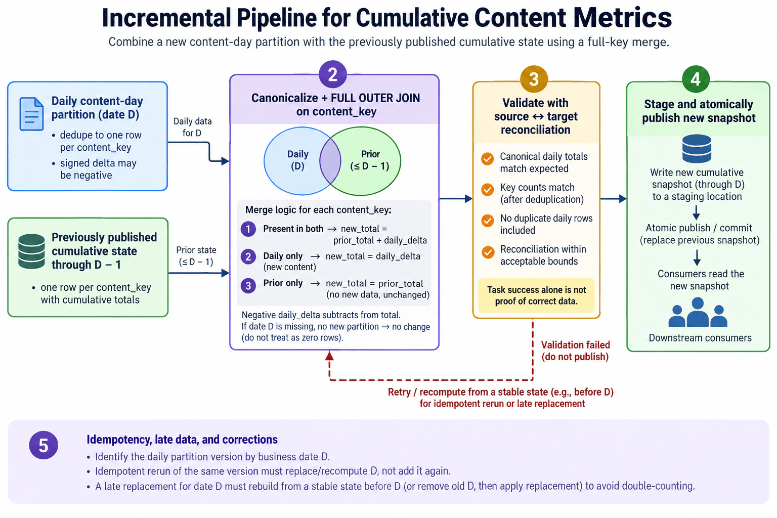
7. Build an incremental pipeline that maintains cumulative content metrics from daily updates.Data PipelinesMediumMeta

Question Details

Combine a newly arrived content-day metric partition with the previously published cumulative state. Use a full-key merge so new content, unchanged content, and content absent from the new day are handled explicitly; define how negative corrections, duplicate daily rows, a late replacement day, missing dates, idempotent reruns, source-to-target reconciliation, and atomic publication affect the cumulative result.

Short Interview Answer (30-60 seconds)

The big picture is to merge each cleaned daily content partition with the cumulative snapshot through the previous day. I would deduplicate the daily input, full-key merge on content_key, apply signed deltas, reconcile the result, then stage and atomically publish the new snapshot. Reruns and late replacements recompute from stable prior state so the same day's contribution is never added twice. The trade-off is extra validation and recomputation in exchange for stronger correctness.

Detailed Explanation

Each day brings a new set of changes for content, and the goal is to keep one trusted running total for every item. Some items already exist, some appear for the first time, and some have no change that day. A change can also reduce an earlier total. Before replacing the published result, the new day's information must be cleaned and checked. Running the same day again must not add it twice. If an older day is replaced later, the totals must be rebuilt from an earlier trusted point so the final result stays correct.

Useful Questions to Ask the Interviewer
  1. Is each daily partition a set of signed changes rather than complete replacement totals?
  2. What rule selects the canonical row when the same content_key appears more than once in a daily partition?
  3. Should a missing business date simply leave the cumulative state unchanged for that date?
  4. What reconciliation conditions must pass before the new cumulative snapshot can be published?
Build an incremental pipeline that maintains cumulative content metrics from daily updates. diagram
How to Explain It in an Interview
1. Read the daily partition and prior cumulative state

I would treat business date D as one batch state transition. The first input is the newly arrived content-day partition for D. After canonicalization, its grain is one row per content_key. Its metric is a signed daily_delta, so positive values increase the running total and negative values reduce it as corrections. The second input is the previously published cumulative state through D - 1, also with one row per content_key. Both inputs flow into the merge step.

2. Canonicalize the daily data

Before joining, I would deduplicate the daily partition to one canonical row per content_key. The diagram does not define how to choose among conflicting duplicate rows, so that rule must come from the source contract. This matters because joining duplicate daily rows could apply a day's contribution more than once. After canonicalization, both inputs have the intended key grain.

3. Full-key merge on content_key

The processing step performs a full outer join on content_key so every key from either side is represented. There are three cases. If the key appears in both inputs, new_total equals prior_total plus daily_delta. If it appears only in the daily partition, it is new content and new_total equals daily_delta. If it appears only in prior state, there is no update for that content on D, so new_total stays prior_total. A negative daily_delta subtracts from the running total. If the entire date D partition is missing, do not create artificial zero rows; there is simply no state change for D.

4. Validate and reconcile the merged result

A completed processing task is not proof that the data is correct. Before publication, I would verify that the canonical daily totals match expectations, key counts are consistent after deduplication, no duplicate daily keys were included, and the cumulative result reconciles with prior state plus the accepted daily changes. The exact acceptable bounds must come from the data contract. If validation fails, publication is blocked.

5. Stage and atomically publish the snapshot

After validation passes, I would write the cumulative snapshot through D to a staging location. The publication step then atomically commits or replaces the previously published snapshot. Downstream consumers read only the committed cumulative state. This keeps partial or failed output hidden and makes the publication boundary part of data correctness.

6. Handle reruns, late replacements, and recovery safely

The business date and daily partition version identify the work being applied. Rerunning the same version for D must replace or recompute D rather than add D again. For a late replacement of D, rebuild from a stable cumulative state before D and apply the replacement, then recompute any later required dates. If the system explicitly supports removing the old D contribution first, that is another valid path before applying the replacement. A failed validation follows the same safe retry or recomputation path, and the existing published snapshot stays visible until a corrected result passes validation.

Technical Approach

1. Read the newly arrived partition for business date D and the published cumulative state through D - 1. 2. Canonicalize the daily partition to one row per content_key. 3. Full outer join daily data and prior state on content_key. 4. For keys in both, compute prior_total + daily_delta; for daily-only keys, use daily_delta; for prior-only keys, keep prior_total. 5. If D is missing entirely, do not manufacture zero rows; leave the cumulative state unchanged for D. 6. Run canonical-total, key-count, duplicate, and source-to-target reconciliation checks. 7. If validation fails, do not publish; retry or recompute from stable state. 8. If validation succeeds, write the cumulative result through D to staging and atomically publish it. 9. For an idempotent rerun or late replacement, recompute from stable prior state so D is not counted twice.

Practical Insights

The benefit is that each normal run only needs the new daily partition and the previously published cumulative state, so the design is easy to reason about. The full-key merge still has to examine keys from both inputs, and the cumulative snapshot can grow as more content appears. Validation adds extra reads and calculations before publication, so delivery is slightly slower. The downside is larger for late replacements because rebuilding from a stable state before D may require reprocessing later dates. We accept this because correctness is more important than publishing a fast but double-counted result. Staging also adds one more write boundary, but it keeps partial output hidden from consumers.

Why Interviewers Ask This

Interviewers ask this to test whether a candidate can reason about a stateful batch pipeline, not just write an aggregation. A strong answer shows judgment about data grain, duplicate daily rows, signed corrections, missing keys, late replacement data, idempotent reruns, reconciliation, failure handling, and atomic publication. It also tests whether the candidate understands that successful task execution is different from proving that the published data is correct.

Common interview mistakes

Common mistakes are using an inner join and silently dropping daily-only or prior-only content, treating a missing daily partition as fabricated zero-valued rows, applying duplicate daily rows more than once, rejecting negative deltas even though they represent corrections, and adding the same partition again during a rerun. Another mistake is publishing before reconciliation passes. A late replacement must not be added on top of the old D contribution; it must rebuild from stable state or explicitly remove the old contribution before applying the replacement. Finally, task completion must not be treated as proof that the cumulative data is correct.

Interview tip

Explain the pipeline as one state transition: canonicalize D, full-key merge it with the state through D - 1, validate the result, then atomically publish through D. Spend extra time on the three merge cases and on why reruns and late replacements must recompute instead of adding the same day's contribution again.

Interviewer may ask next
How would the design change if a corrected partition for an old business date arrives after several newer dates have already been published?

I would keep the same architecture but use the late-replacement recovery path. The requirement changes because an historical day's contribution must be replaced without double-counting it. I would start from a stable cumulative state before the corrected date, process the replacement partition for that date, and then reapply any later required daily partitions until the current cumulative state is reconstructed. The one-row-per-content_key contract and the same full-key merge rules remain unchanged. Each rebuilt result still goes through duplicate checks and source-to-target reconciliation. Downstream consumers continue reading the existing published snapshot until the reconstructed version passes validation and is atomically committed. If the storage model explicitly supports removing the old day's contribution first, that can be used before applying the replacement instead. The main downside is recovery cost, because one historical correction may force several later dates to be recomputed.

What should happen if validation fails after the merged cumulative snapshot has already been written to staging?

I would leave the currently published cumulative snapshot unchanged. The affected component is the validation and publication boundary, not the merge logic. Because the new result is only in staging, a failed reconciliation must block the atomic publish step. I would retry or recompute using the same stable prior cumulative state and the canonical daily partition. The business date and partition version keep that repeated work idempotent, so D is recomputed rather than added again. The same canonical-total, key-count, duplicate, and source-to-target reconciliation checks must pass before publication is attempted again. Partial or failed staged output remains invisible to downstream consumers, so the trusted snapshot stays available during recovery. The main downside is higher delivery latency when validation fails, but that delay is preferable to exposing an incomplete or incorrect cumulative result.

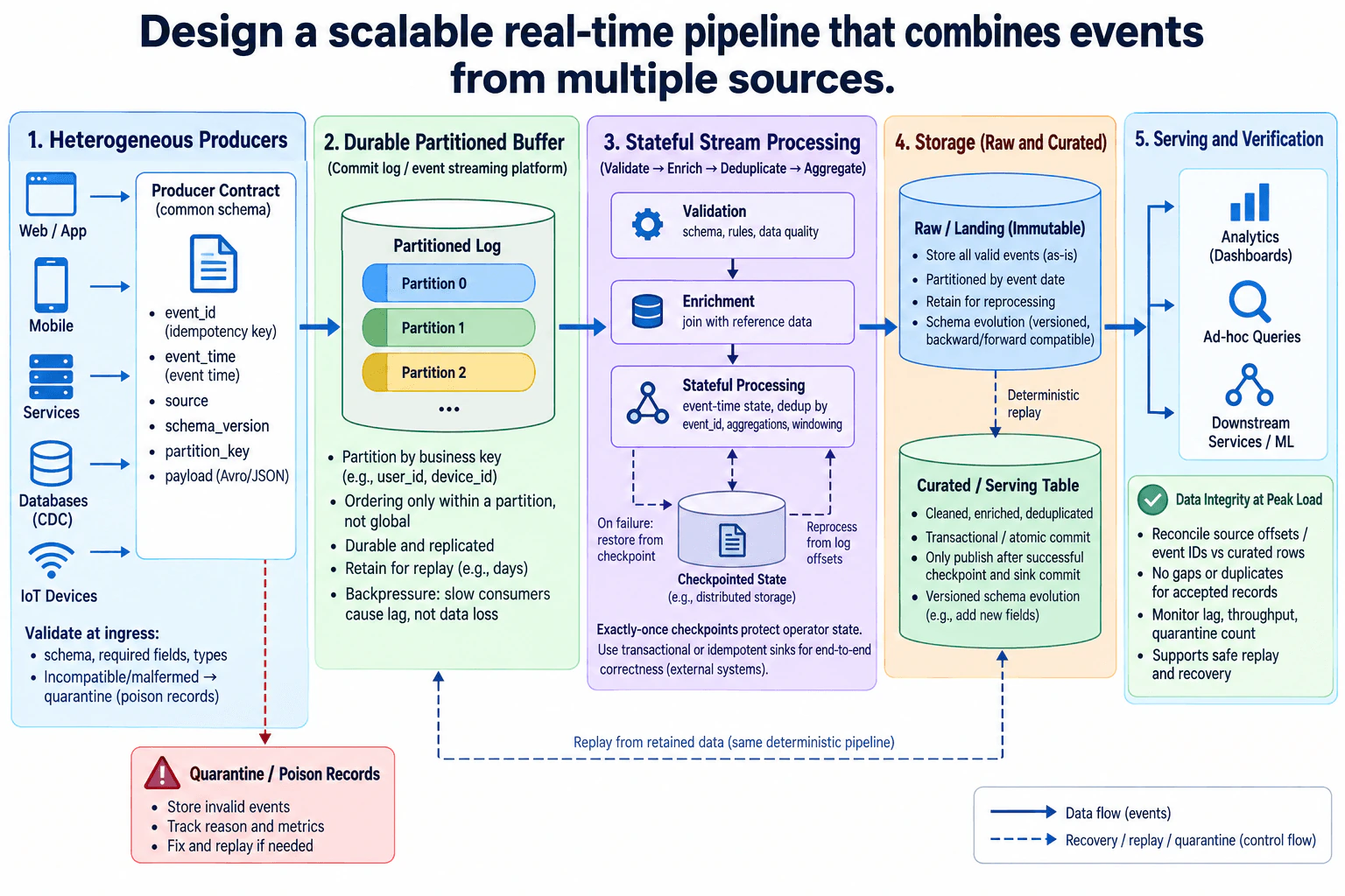
8. Design a scalable real-time pipeline that combines events from multiple sources.Data PipelinesHardMeta

Question Details

Specify producer contracts, durable buffering, partitioning, validation, enrichment, stateful processing, raw and curated storage, and serving for heterogeneous real-time sources. Include ordering scope, duplicate delivery, schema evolution, backpressure, checkpoint and sink consistency, poison records, replay, worker failure, and evidence that data integrity is preserved at peak load.

Short Interview Answer (30-60 seconds)

I would normalize all sources to one versioned event contract, validate them, and write accepted events to a durable log partitioned by a business key. Stateful workers then validate, enrich, deduplicate by event_id, and process by event time. Durable checkpoints support recovery, while transactional or idempotent sinks prevent retries from creating duplicate business results. Raw data remains available for replay, poison records are quarantined, and source progress is reconciled with curated output. The trade-off is extra state, retention, and coordination for stronger correctness.

Detailed Explanation

The goal is to combine live information from several systems without silently losing, repeating, or mixing up records. Every source sends the same basic identifying information so the pipeline knows what happened, when it happened, where it came from, which version of the record format it uses, and whether the record has already been seen. Bad records are separated instead of disappearing. Good records are stored safely, processed into useful output, kept in original and cleaned forms, and checked against what arrived so mistakes can still be found during the busiest periods.

Useful Questions to Ask the Interviewer
  1. Which business key should define the ordering boundary: user, device, or another entity?
  2. How long must raw events and the durable log remain available for replay?
  3. How late may an event arrive before the business stops updating an event-time result?
  4. What consistency guarantee must downstream consumers observe when curated results become visible?
Design a scalable real-time pipeline that combines events from multiple sources. diagram
How to Explain It in an Interview
1. Standardize and validate producer events

I would start with one producer contract shared by Web / App, Mobile, Services, Databases using CDC, and IoT Devices. Each event contains event_id, event_time, source, schema_version, partition_key, and a payload. The payload may use an agreed serialization such as Avro or JSON, as shown in the diagram.

event_id is the idempotency and deduplication key. event_time means when the source event occurred, which is different from processing time, when the pipeline happens to handle it. schema_version lets producers and consumers manage schema evolution explicitly.

At ingress, I validate schema, required fields, and types. An incompatible or malformed record moves to Quarantine / Poison Records with its failure reason and metrics. It is not silently dropped or allowed to corrupt downstream state. After correction, it can be replayed deliberately.

2. Buffer durably and partition for scalable ordering

Accepted events enter the Durable Partitioned Buffer, represented as a replicated commit log or event-streaming platform. I partition by a business key such as user_id or device_id. Related events with the same key therefore go to the same partition, so the system can preserve order within that partition. I would not claim global ordering across all partitions.

The durable buffer separates producer speed from consumer speed and retains events for replay. If processors temporarily cannot keep up, consumer lag grows instead of the pipeline intentionally discarding accepted records, assuming retention and capacity have not been exhausted. More partitions can increase parallelism, but partition count, key skew, worker capacity, and sink capacity all limit useful scaling.

3. Validate, enrich, deduplicate, and process by event time

The Stateful Stream Processing stage follows the diagram's order: Validate, Enrich, Deduplicate, then Aggregate. Validation applies schema, rules, and data-quality checks. Enrichment joins each event with the required reference data. Stateful processing then keeps the information needed to deduplicate by event_id, aggregate records, and maintain event-time windows.

Duplicate delivery is different from duplicate business output. An event may be delivered or processed again after a retry or recovery, but deduplication state and the idempotency key prevent the same accepted event from producing another logical result.

For out-of-order or late events, the event-time logic needs a defined late-data policy, normally expressed with a watermark or equivalent event-time progress rule. The exact lateness threshold is a business requirement and is not specified in the diagram, so I would not invent a value. Records that are still within the allowed late-data policy update the appropriate state or window; records beyond that policy require the agreed correction or replay behavior.

4. Checkpoint state and recover safely from worker failure

Processing state is persisted in durable Checkpointed State. If a worker fails, replacement processing restores state from the latest consistent checkpoint and reprocesses retained log records from the corresponding progress point. This lets stateful calculations continue without trusting volatile worker memory.

A checkpoint protects processing-engine state, but it does not automatically make every external business result exactly once. The destination must also support a transactional commit or an idempotent write strategy that is consistent with processing progress. Progress must not be treated as safely complete before the supported sink commit boundary.

This distinction is important: transport or checkpoint semantics describe how records are delivered and recovered, while business correctness means a retry still produces one intended logical result.

5. Keep replayable raw data and safely publish curated data

The Storage boundary contains Raw / Landing and the Curated / Serving Table. Raw / Landing keeps valid events as an immutable history, partitioned by event date, so they are available for reprocessing and audit. Schema versions remain attached to the data so compatible evolution can be interpreted deliberately rather than guessed.

The Curated / Serving Table contains cleaned, enriched, and deduplicated output. The diagram requires transactional or atomic publication behavior and says output becomes visible only after the successful checkpoint and sink commit. That publication boundary prevents consumers from observing known partial results.

Schema evolution must also be versioned. Compatible changes, such as adding supported fields, can be introduced through the agreed contract. An incompatible schema should be rejected or quarantined rather than silently reinterpreted.

6. Replay, serve, and prove integrity at peak load

Retained data supports deterministic replay through the same processing logic. Replay is different from a normal worker retry: a retry repeats failed processing from recovery state, while replay intentionally reprocesses retained historical events. Poison records can be corrected and deliberately replayed rather than skipped.

Curated data is then served to Analytics dashboards, Ad-hoc Queries, and Downstream Services / ML, matching the diagram.

At peak load, I would prove data integrity rather than infer it from healthy workers. I would reconcile source offsets or accepted event_id values against curated rows, verify that accepted records have no unexplained gaps or duplicates, and monitor lag, throughput, and quarantine count. Rising lag shows that consumers are falling behind; quarantine growth shows rejected inputs; reconciliation reveals correctness failures that ordinary task-health metrics can miss.

Technical Approach
  1. Define one versioned producer contract containing event_id, event_time, source, schema_version, partition_key, and payload.
  2. Validate required fields, types, and schema compatibility at ingress; route malformed or incompatible events to quarantine.
  3. Append accepted events to a durable replicated log partitioned by the selected business key.
  4. Consume partitions with stateful processing that validates, enriches, deduplicates by event_id, and maintains event-time aggregation or window state.
  5. Apply a defined event-time lateness policy without inventing an unsupported threshold.
  6. Persist processing state in durable checkpoints and restore from a consistent checkpoint after worker failure.
  7. Store valid events in immutable Raw / Landing storage, partitioned by event date, for replay and reprocessing.
  8. Publish cleaned, enriched, and deduplicated output to the Curated / Serving Table through a transactional or idempotent sink boundary consistent with checkpoint progress.
  9. Replay retained data through the same deterministic processing logic when recovery or historical reprocessing is required.
  10. Reconcile source offsets or accepted event IDs against curated rows while monitoring lag, throughput, and quarantine count.
Practical Insights

The benefit is that partitioning lets independent keys be processed in parallel while the durable log absorbs temporary differences between producer and consumer speed. The downside is more coordination and stored state. More partitions can raise throughput, but they also increase scheduling and checkpoint overhead and cannot solve a slow destination or a hot key. Longer retention makes replay safer, but it costs more storage. Keeping deduplication and event-time state longer handles more delayed or repeated events, but increases memory or state-store cost. Transactional or idempotent publication adds sink complexity, but it makes retries safer. We accept these costs because this design values correct, recoverable results during peak load rather than only minimum latency.

Why Interviewers Ask This

This question tests whether a candidate can preserve correctness while designing a real-time pipeline that scales. Interviewers want to see clear producer contracts, partition-scoped ordering, duplicate handling, event-time reasoning, checkpoint recovery, safe sink publication, poison-record handling, replay, and peak-load verification. It also tests whether the candidate understands that message-delivery semantics do not automatically guarantee correct business results and can discuss the trade-offs among throughput, state size, retention, latency, and reliability.

Common interview mistakes

Common mistakes are claiming global ordering when the design only provides ordering inside a partition; confusing event time with processing time; ignoring late events; treating duplicate delivery as duplicate-free business output without event_id deduplication; claiming that checkpoints alone guarantee exactly-once results in every external sink; advancing progress before a safe sink commit; dropping poison records instead of quarantining them; failing to retain raw data for deterministic replay; and treating worker health as proof that no data was lost or duplicated. Another mistake is assuming that adding workers always solves peak load without checking partition count, key skew, state size, checkpoint cost, and destination write capacity.

Interview tip

Explain the design left to right and keep calling out the correctness boundaries: common versioned contract, partition-scoped ordering, durable buffering, event-time state, deduplication, checkpoint recovery, safe sink commit, immutable raw replay, poison-record quarantine, and reconciliation. Explicitly separate delivery guarantees from business-result correctness. If you use the term exactly once, state exactly which boundary provides that guarantee and what the sink must do to preserve it.

Interviewer may ask next
What would you change if peak traffic suddenly became several times higher and consumer lag kept increasing?

I would keep the same architecture and first find the actual bottleneck instead of blindly adding workers. The changed requirement is higher sustained throughput while keeping the same partition-ordering and correctness rules. I would inspect lag and throughput around the Durable Partitioned Buffer, then check whether there are enough independent partitions for additional stateful workers to process in parallel. The partition key must remain consistent with the required business ordering scope; casually changing it could reorder related events.

I would also inspect worker CPU and state pressure, checkpoint duration, enrichment capacity, key skew, and Curated / Serving Table write capacity. If the destination is saturated, adding processors upstream only moves the backlog. Retained events remain in the durable buffer while processors catch up, subject to retention and available capacity.

Checkpoint recovery, event_id deduplication, quarantine behavior, and transactional or idempotent publication remain unchanged. After scaling, I would reconcile source progress or accepted event IDs against curated rows and inspect gaps, duplicates, lag, throughput, and quarantine count. The downside is higher compute, state, checkpoint, and coordination cost.

How would you handle a bug in enrichment logic that produced incorrect curated results for a period of time?

I would use the existing Raw / Landing retention and deterministic replay path instead of building a separate correction pipeline. The changed requirement is to recompute affected historical events with corrected enrichment logic without creating duplicate curated business results. I would identify the affected event range and schema versions, correct the enrichment logic, and replay the retained raw events through the same validation, enrichment, deduplication, and stateful-processing path.

The replay keeps the original event_id, event time, partitioning rules, and schema-version meaning. The Curated / Serving Table still uses a transactional or idempotent publication boundary so repeated processing produces the intended logical result rather than blindly appending duplicates. Poison records remain quarantined rather than being silently skipped.

After replay, I would reconcile the affected source progress or accepted event IDs against corrected curated rows and check for unexplained gaps and duplicates before treating the repair as complete. Live processing keeps the same architecture. The main downside is that replay consumes buffer, compute, state, and sink capacity, so historical reprocessing must be controlled so it does not overwhelm the live path.

9. Choose a platform layout for real-time online-learning metrics.Cloud Data PlatformsEasyMeta

Question Details

Select durable event storage, stream-processing compute, a historical analytical table, and a low-latency serving layer for learner progress and completion metrics. State freshness and retention goals, query patterns, update frequency, schema ownership, failure recovery, and how the design balances storage cost against dashboard latency.

Short Interview Answer (30-60 seconds)

I would use Kafka for durable replayable events, Flink for continuous learner-metric computation, Pinot for recent low-latency dashboard reads, and Iceberg for long-term analytics. The main trade-off is keeping latency-sensitive data in Pinot while retaining longer history in lower-cost analytical storage.

Detailed Explanation

Learners, instructors, analysts, dashboards, and APIs need progress and completion metrics that are both fresh and historically useful. Several producers generate events continuously, so a one-off pipeline is not enough. The platform separates durable event retention, stateful stream processing, low-latency serving, checkpoint recovery, and historical analytical storage. It prioritizes seconds-level freshness for recent metrics, a dashboard-query target of at most one second, Kafka replay within a 7–30 day retention window, and months-to-years history in Iceberg. This keeps recent reads fast without forcing all retained history into the low-latency serving layer.

Useful Questions to Ask the Interviewer
  1. What event volume and growth should the streaming path handle?
  2. Which dashboard and Metrics API queries are the most latency-sensitive?
  3. How much historical data must remain queryable beyond the stated months-to-years retention goal?
  4. What availability and recovery objectives should apply to learner-progress and completion metrics?
  5. Are additional producer or consumer teams expected to use the same shared platform?
Choose a platform layout for real-time online-learning metrics. diagram
How to Explain It in an Interview
1. Set the freshness, retention, and query goals

The design has two read patterns. Recent learner progress and completion metrics need seconds-level freshness and interactive access. Historical cohort and time-window analysis needs much longer retention. Kafka keeps source events for 7–30 days, Flink updates derived metrics continuously, Pinot serves recent latency-sensitive aggregates, and Iceberg retains historical data for months to years.

The Pinot-to-consumer path has a dashboard-query design target of at most one second. That is a target for this design, not an unconditional platform guarantee.

2. Define the producer and consumer boundaries

The producer side contains the web application, mobile application, backend services, and third-party integrations. Example events include lesson views, quiz attempts, video plays, assessments, enrollments, completions, course-catalog updates, and user updates. These events enter Kafka using the event contract shown as Avro or JSON.

The consumer side contains real-time dashboards, a Metrics API, and data analysts. Dashboards consume learner progress and completion metrics. The Metrics API supports course and learner lookups. Iceberg provides historical data for analytical patterns such as cohort and time-window analysis.

3. Keep schema ownership explicit

The learning-analytics data product team owns the event schema. That ownership matters because Kafka, Flink, Pinot, Iceberg, dashboards, and analytical consumers depend on compatible field meanings.

The diagram does not define a separate provisioning portal, identity service, tenant model, region boundary, or dedicated control-plane system. I would not invent those components. The visible architecture is mainly the production data plane, with schema ownership acting as the explicit governance contract shown in the design.

4. Use Kafka as the durable event-storage and replay boundary

Kafka receives events from the producers and stores them in a partitioned, append-only, replayable stream. Its configured retention goal in this design is 7–30 days.

Kafka is the source for normal Flink consumption and for replay after a processing failure. It is not the long-term analytical table and it is not the dashboard-serving database. If processing falls behind or fails, retained Kafka events give Flink a bounded replay window.

Operationally, I would watch stream lag and whether the required replay history still fits inside the configured retention period.

5. Use Flink for continuous stateful computation

Flink consumes the real-time Kafka stream and computes learner progress and completion metrics. It maintains state because progress is derived across multiple events rather than from only one independent record.

Flink publishes a stream of aggregates and updates to Pinot for recent serving. It also writes processed events to the Iceberg analytical table for historical analysis.

The diagram states exactly-once state consistency for Flink. I would keep that claim scoped to the processing-state boundary and would not automatically describe every external sink as providing end-to-end exactly-once business results.

6. Persist Flink checkpoints separately

Flink writes checkpoint state to durable checkpoint storage. That path is different from Kafka event retention. A checkpoint saves processing state; Kafka retains business events.

After a Flink failure, the processor restores its latest checkpoint and then consumes retained Kafka events as needed to continue from the recovered stream position. The recovery flow therefore combines state restore with event replay instead of treating checkpoint storage as an event source.

Useful health signals are checkpoint success, checkpoint duration, stream lag, and whether recovered outputs reconcile with the expected learner metrics.

7. Serve recent metrics from Pinot

Pinot is the low-latency serving layer. Flink sends recent learner and course progress and completion aggregates to it continuously.

Pinot supports the latency-sensitive consumer path. The architecture assigns it recent, high-value metrics and uses a dashboard-query target of at most one second. Examples include current learner progress and completion rates.

If Pinot falls behind, the consumer-visible problem is stale or slower real-time metrics. That should be detected through ingestion freshness and query-latency signals rather than silently presenting stale data as current.

8. Keep historical analytical data in Iceberg

Flink also sinks processed events into an Apache Iceberg historical analytical table. The diagram assigns Iceberg months-to-years retention and shows snapshots, schema and partition evolution, compaction, and cohort or time-window history.

This makes Iceberg the long-term analytical boundary rather than the low-latency serving layer. Periodic compaction keeps continuously written historical data efficient to query over time.

This separation is important for cost. The platform does not need to keep all historical detail in Pinot merely to preserve years of analytical history.

9. Explain the normal and recovery flows separately

The normal path is producers to Kafka, Kafka to Flink, Flink to Pinot for recent aggregates, and Flink to Iceberg for historical processed data. Pinot then serves the low-latency consumer path.

The dashed Kafka-to-Flink arrow is a recovery flow, not a second normal data path. After failure, Flink restores checkpointed state and replays retained Kafka events. If the required source events have aged out of the 7–30 day Kafka window, the shown recovery path alone cannot replay them.

The diagram does not claim multi-region failover, unlimited replay retention, or a separate raw archival store, so I would not add those guarantees.

10. State the cost-versus-latency trade-off

The main design decision is to keep recent latency-sensitive aggregates in Pinot while keeping longer-term historical data in Iceberg. Pinot is used where interactive dashboard latency matters. Iceberg is used where long retention and analytical access matter more than serving every query through the real-time store.

Kafka retention is also bounded at 7–30 days instead of making Kafka the permanent history system. This saves the serving and event layers from carrying every historical requirement, but it adds operational complexity because Kafka, Flink, checkpoint storage, Pinot, and Iceberg must be operated as distinct platform components.

Technical Approach
  1. Separate the requirements into durable ingestion, continuous stateful computation, recent low-latency serving, historical analytics, and recovery.
  2. Send producer events to Kafka using the Avro or JSON event contract.
  3. Retain Kafka events for 7–30 days so recent source data remains replayable.
  4. Consume Kafka continuously with Flink and compute learner progress and completion metrics.
  5. Persist Flink state to durable checkpoint storage.
  6. Publish recent aggregates and updates from Flink to Pinot for seconds-level freshness and low-latency consumer queries.
  7. Write processed events from Flink to Iceberg for months-to-years analytical history.
  8. Use Pinot for current learner and course metric reads and Iceberg for cohort and time-window historical analysis.
  9. Keep schema ownership with the learning-analytics data product team.
  10. On Flink failure, restore the latest checkpoint and replay retained Kafka events.
  11. Monitor stream lag, checkpoint health, Pinot freshness and query latency, and Iceberg maintenance.
  12. Keep recent latency-sensitive data in Pinot and longer history in Iceberg to balance serving cost against dashboard latency.
Practical Insights

The streaming path grows with incoming event volume because Kafka must retain events and Flink must process them continuously. More state can increase checkpoint size and recovery time. Pinot cost and capacity grow with recent retained aggregates, ingestion work, and interactive query concurrency. Iceberg storage grows with historical retention, and continuous writes create maintenance work such as compaction. Network use grows as events move from producers to Kafka and from Flink to its serving and historical sinks. The first practical bottlenecks to watch are Kafka or Flink lag, slow or growing checkpoints, Pinot freshness or query latency, and inefficient Iceberg file layouts. No precise throughput or capacity number is assumed because the question does not provide one.

Why Interviewers Ask This

Interviewers want to see whether a candidate can translate freshness, retention, query, recovery, ownership, and cost requirements into clear platform boundaries. The key judgment is recognizing that durable event storage, stateful processing, low-latency serving, and historical analytics have different responsibilities and should not be collapsed into one system.

Common interview mistakes

A common mistake is putting both real-time dashboard serving and years of history into one datastore even though those workloads have different latency and cost needs. Another is treating Kafka as the permanent historical analytical store instead of a replayable event-retention boundary. Candidates also confuse checkpoints with event backups: checkpoints restore Flink processing state, while Kafka supplies retained business events for replay. Another mistake is reversing the recovery flow or describing the dashed Kafka-to-Flink recovery arrow as the normal data path. It is also incorrect to claim that Flink's exactly-once state consistency automatically proves end-to-end exactly-once results for every sink. Finally, do not invent a self-service portal, tenant model, identity system, multi-region failover, or control-plane service that the approved diagram does not contain.

Interview tip

Explain the design by access pattern. Start with why recent metrics go to Pinot and long history goes to Iceberg, then explain Kafka replay and Flink checkpoint restore as separate recovery mechanisms. End with the trade-off: spend low-latency resources on recent data and keep long-term history in the analytical table.

Interviewer may ask next
What happens if Flink is unavailable long enough that required events are no longer retained in Kafka?

The normal recovery path has a clear limit. Flink can restore its latest checkpoint and replay Kafka only while the required events still exist inside the configured 7–30 day retention window. If they have expired, the diagram does not provide a separate raw-event archive that guarantees full replay. I would first check whether the required metric can be safely recomputed from the historical data already written to Iceberg and then reconcile the rebuilt result before republishing it. If Iceberg does not contain enough source detail, the current architecture has a recovery gap for that interval. That would justify reconsidering Kafka retention or adding a raw archival layer in a future design, but that extra store is not part of the approved architecture.

How would you handle a request to expose a much larger historical window through the same low-latency dashboards?

I would first identify which historical aggregates truly need the dashboard latency target. The current architecture deliberately keeps recent latency-sensitive aggregates in Pinot and long-term history in Iceberg. If a larger interactive window is required, I would extend only the necessary aggregate range in Pinot and measure the effect on serving storage, ingestion work, and query capacity. Iceberg would remain the long-term historical analytical table. This changes the cost-versus-latency boundary without changing the basic architecture. If the expanded serving footprint becomes too expensive or operationally heavy, older queries should remain on the Iceberg analytical path instead of forcing every historical record into Pinot.

10. Design a lakehouse or warehouse architecture for billions of Meta events per day.Cloud Data PlatformsMediumMeta

Question Details

Choose object storage, transactional table format or warehouse tables, distributed transformation compute, catalog, orchestration, and serving components. Cover raw retention, partition and file management, concurrent writes, interactive query isolation, late corrections, backfills, access controls, observability, and cost attribution at billion-event daily scale.

Short Interview Answer (30-60 seconds)

I would build a shared S3-backed Delta Lake platform with separate control and data planes. Kafka ingests events, Spark transforms Bronze into Silver and Gold tables, and Databricks SQL serves consumers. The main trade-off is shared efficiency versus stronger workload isolation and governance overhead.

Detailed Explanation

Meta engineering teams need a reusable way to ingest, transform, govern, and serve very large event streams without rebuilding the same foundation for every product. One-off pipelines are not enough because raw retention, late corrections, concurrent writes, backfills, access control, query isolation, observability, and cost ownership must behave consistently across many datasets. I would use a lakehouse on object storage with transactional Delta tables, Kafka for event ingestion, and Spark for distributed processing. I would keep orchestration, metadata, identity, and policy in a separate control plane so production records remain in the data plane.

Useful Questions to Ask the Interviewer
  1. What freshness targets do the main consumers need: near-real-time, hourly, or batch?
  2. Which event classes contain sensitive data that need stronger dataset, row, or column controls?
  3. What query patterns dominate the serving layer: exploratory SQL, dashboards, APIs, feature-store access, or scheduled reporting?
  4. Is cross-Region recovery required for the whole platform, or is S3 replication needed only for selected datasets?
  5. How much compute isolation is required between teams for transformation jobs, backfills, and interactive SQL?
  6. Are producer schemas centrally governed, or do domain teams own schema evolution within platform guardrails?
Design a lakehouse or warehouse architecture for billions of Meta events per day. diagram
How to Explain It in an Interview
1. Goals, users, and ownership

The platform supports many Meta event producers and many downstream consumers. Event sources in the diagram include Facebook, Instagram, WhatsApp, Meta Quest, and other Meta products. Producer engineering teams own the meaning and correctness of their event contracts. The shared platform supplies reusable ingestion, object storage, transactional tables, distributed compute, orchestration, governance, serving, monitoring, lifecycle management, and cost attribution.

Consumers include analysts, ML and product teams, BI tools, feature-store or internal-service workloads, and data APIs. This is a platform because these capabilities are reused across many pipelines and data products rather than being rebuilt for each dataset.

2. Separate the control plane from the production data plane

The control plane contains the self-service portal or CLI, Airflow orchestration, Unity Catalog governance, and SSO/IAM-based identity and policy controls. Teams submit desired configuration through templates with validation and quotas. Airflow stores workflow definitions and coordinates schedules, retries, and bounded backfills. Unity Catalog stores metadata, classification, lineage, ownership, and authorization information. It does not store production event records.

The data plane carries the actual events, table files, Spark transformations, and query traffic. The purple control-flow arrows represent schedules, configuration, policies, and metadata. They do not carry business records. Keeping these planes separate reduces the blast radius of control-plane failures and avoids putting administrative services in the event-processing path.

3. Ingest events through Kafka

The normal streaming path sends product events into Kafka. Kafka provides a partitioned, replicated log so ingestion can scale horizontally across partitions and consumers. Producers can use idempotent and transactional producer behavior where appropriate, but I would not call the whole platform end-to-end exactly-once because final correctness also depends on consumer processing, checkpoints, transformation logic, and Delta commits.

The diagram also shows a batch backfill path entering the ingestion boundary. A backfill is bounded historical reprocessing, not a separate permanent architecture. Airflow controls the historical range, while the processing jobs must remain idempotent so reruns do not create incorrect duplicate results.

If downstream processing slows, Kafka provides a durable buffering boundary. Operators watch ingestion health and consumer lag. Recovery resumes from durable offsets or checkpoints rather than silently skipping records.

4. Land immutable raw events in Bronze on S3

Ingestion consumers persist the raw event stream into the Bronze zone on Amazon S3. Bronze contains immutable events and is partitioned by event date, for example dt=YYYY-MM-DD. The diagram also calls out domain-aware partitioning as a possible scale practice when it matches the workload.

Raw data is retained according to lifecycle policy rather than a hard-coded duration. This gives the platform a replay source for late corrections, logic changes, and historical recomputation. The trade-off is extra storage and lifecycle-management cost.

S3 is Regional object storage. Cross-Region replication is optional and must be configured explicitly. Replicating objects to another Region does not, by itself, create complete multi-Region platform failover because Kafka, Airflow, Spark compute, catalog metadata, identity, and serving also have recovery dependencies.

5. Use Delta Lake for transactional Bronze, Silver, and Gold tables

The S3-backed tables use Delta Lake as the transactional table format. Delta supplies ACID table commits, versioned history, MERGE operations, schema evolution mechanisms, and concurrency control around conflicting table updates.

Silver contains cleaned data. Spark de-duplicates records when required by the data contract, enforces the expected schema, handles late-arriving data, and applies upserts or MERGE operations for corrections.

Gold contains curated analytics models, aggregations, and reusable data products optimized for consumer queries. Consumers should see only successfully committed table versions rather than partially written logical outputs.

Concurrent writers do not need to be globally serialized. Delta uses transactional commit rules and optimistic concurrency behavior. Non-conflicting operations can proceed, while conflicting writes can fail and must be retried or coordinated by the owning workload. This is more accurate than saying every concurrent write automatically succeeds.

6. Transform with Spark on Databricks

Spark on Databricks owns the distributed transformations. It reads raw or intermediate Delta tables, performs batch or streaming transformations, and writes new committed versions of Silver and Gold tables. It also handles incremental processing, backfills, and data-quality work.

Airflow schedules this work but does not perform the transformations itself. That responsibility stays with Spark.

At billion-event daily scale, the processing layer needs enough parallelism to keep up with incoming data and historical jobs. Likely bottlenecks include skewed partitions, large shuffles, small-file growth, conflicting table updates, and backfills competing with normal processing. These problems are detected through job metrics, logs, freshness signals, and data-quality checks.

If a Spark job fails before a Delta commit, the logical table update should not be treated as published. Airflow records the failed run. Operators inspect the failure, correct deterministic issues, and retry or backfill the affected range. Reconciliation and quality checks verify the recovered output before consumers treat it as healthy.

7. Manage partitions and files as part of normal platform operations

Partitioning is used to reduce unnecessary scans and to organize large tables, but partitioning by too many high-cardinality values can create excessive metadata and small files. The diagram uses event-date partitioning and allows domain-aware partitioning when appropriate.

Streaming and incremental writes can create many small files. The platform therefore compacts small files and tunes target file size according to the workload. Lifecycle jobs also manage retention and table maintenance. These background operations consume compute, so the platform has to balance freshness against file efficiency and maintenance cost.

8. Isolate interactive SQL from heavy transformation workloads

Databricks SQL is the interactive query-serving layer. Interactive SQL runs on separate SQL warehouses rather than sharing the same compute pool as Spark transformations and large backfills.

This protects dashboards and exploratory queries from noisy neighbors. Heavy historical recomputation can consume transformation resources without directly starving interactive query compute. It also makes interactive query usage easier to meter separately from transformation work.

Consumers include BI tools such as Tableau and Looker, data APIs for feature-store or internal-service workloads, and analysts, ML teams, and product teams. These consumers read governed curated data rather than reaching directly into uncontrolled raw files.

9. Enforce access through identity, catalog policy, and audit controls

SSO and IAM establish human and workload identity. Unity Catalog provides the governed metadata and authorization boundary. RBAC and ABAC rules can control access to cataloged objects, while lineage and classification help determine where sensitive data exists and which downstream consumers may be affected by a change.

The important point is that metadata or classification labels alone do not protect data. Authorization must be enforced when users and workloads access governed objects. Audit records provide evidence of access and policy activity.

The design does not assume a specific regulatory regime, residency rule, masking requirement, or encryption-key model because the question does not provide one.

10. Observe platform health and data health separately

The observability layer collects metrics, logs, lineage, pipeline state, data-quality signals, freshness, and incident information. Different failures have different owners.

A failed Spark environment, unavailable Kafka dependency, or unhealthy SQL service is a shared platform problem. A bad producer schema or incorrect business transformation is usually a domain-data problem. Both should be visible through common observability, but alerts should route to the correct owner.

Ingestion monitoring includes throughput and lag. Transformation monitoring includes failed jobs, run duration, retries, and freshness. Data-quality monitoring covers schema and expected data behavior. Query monitoring covers SQL failures, concurrency pressure, and degraded consumer experience.

11. Attribute shared-platform cost by team or data product

The platform tags and reports storage, compute, and query usage by team or data product. This covers S3 storage, Spark transformation work, Databricks SQL usage, and other attributable platform consumption.

That allows showback or chargeback without forcing every team onto fully dedicated infrastructure. It also makes expensive backfills, poorly organized tables, and unusually heavy query workloads visible to the team responsible for them. I would not invent a savings percentage or a specific billing formula.

12. Handle late corrections and backfills through the same architecture

Late events follow the normal ingestion and storage path. Spark applies correction logic to Silver or Gold tables, often with Delta MERGE or another transactional update. The correction becomes a new committed table version.

For a historical logic change, Airflow schedules a bounded backfill. Spark rereads the retained Bronze partitions for the affected range, recomputes the target tables, and publishes corrected Delta versions. Backfill concurrency should be limited so historical work does not starve normal processing.

After the backfill, the owner reconciles counts, schema expectations, and business-level checks before marking the data healthy. A retry reruns failed work. A replay rereads retained events. A backfill intentionally recomputes a historical range. Those operations should not be treated as synonyms.

13. Design reliability around each dependency

Kafka protects the ingestion boundary with a replicated log. S3 supplies durable Regional object storage. Delta provides transactional table commits. Airflow persists orchestration state. Unity Catalog carries important metadata and policy state. Databricks SQL supplies isolated query compute.

Each dependency needs its own health signal and recovery path. If interactive SQL is unavailable, ingestion and transformation can continue while query consumers are degraded. If Spark processing fails, Kafka and Bronze can continue retaining data until processing resumes. If governance services are unavailable, the platform should not bypass access policy just to keep serving queries.

Recovery order depends on the failed components. Restore or recover critical control-plane metadata and identity dependencies before opening governed serving paths. Then resume transformations from durable Kafka positions or retained Bronze data, validate table state, and finally restore consumer access. No recovery-point or recovery-time objective is invented because none is supplied.

14. Evolve and adopt the platform incrementally

Teams should onboard through the self-service path in stages rather than move every dataset at once. A producer defines ownership, schema, retention, access rules, and cost attribution. The team then lands raw data, builds Silver and Gold tables, validates downstream consumers, and cuts over when the new output reconciles with the previous path.

Historical data can be backfilled from retained Bronze data when needed. Templates, schema rules, policies, and processing runtimes should be versioned so changes can be introduced deliberately. Breaking changes need a migration path rather than silently invalidating consumers.

The escape hatch for exceptional workloads should remain explicit. A workload that does not fit Kafka, Delta, Spark, or Databricks SQL can use a separately reviewed design rather than weakening the default platform for every team.

15. Main trade-offs

The first trade-off is shared efficiency versus isolation. Shared ingestion, storage, catalog, and platform services reduce duplicated engineering work, while separate SQL warehouses protect interactive consumers from heavy transformation jobs.

The second is raw retention versus cost. Bronze retention makes replay and correction possible, but lifecycle policy is needed so storage does not grow without control.

The third is domain autonomy versus centralized governance. Domain teams retain ownership of event semantics and curated data products, while the shared platform enforces identity, catalog, validation, observability, and cost standards.

The fourth is freshness versus file and compute efficiency. More frequent writes can improve freshness but increase small-file creation and background compaction work.

The fifth is operational portability versus managed integration. The selected design uses Databricks-specific serving and governance components, which simplify integration with Delta and Spark but increase dependence on that managed platform.

Technical Approach
  1. Define producer teams, consumers, data products, and ownership boundaries.
  2. Separate a control plane for self-service, Airflow scheduling, Unity Catalog metadata, identity, policy, quotas, and audit from a production data plane that carries events and queries.
  3. Ingest streaming events through partitioned, replicated Kafka.
  4. Persist immutable raw events into S3-backed Bronze Delta tables with lifecycle-based retention.
  5. Use Spark on Databricks to build cleaned Silver tables and curated Gold data products.
  6. Use Delta transactions, MERGE, schema-evolution mechanisms, and optimistic concurrency behavior for late corrections and concurrent writes.
  7. Partition tables according to workload needs and compact small files.
  8. Serve governed curated tables through separate Databricks SQL warehouses, BI tools, data APIs, and internal consumers.
  9. Enforce SSO/IAM, RBAC/ABAC, catalog policy, classification, lineage, and audit.
  10. Monitor ingestion health, Spark jobs, data quality, freshness, lineage, and interactive queries.
  11. Attribute storage, Spark compute, and SQL usage by team or data product.
  12. Use Airflow and retained Bronze data for bounded backfills, recomputation, and reconciliation.
  13. Recover each dependency independently and never treat S3 cross-Region replication alone as complete platform disaster recovery.
Practical Insights

The platform scales at several independent boundaries. Kafka adds partitions to spread event ingestion. Spark adds distributed compute to process larger datasets and more simultaneous transformations. S3 absorbs long-term data growth, while Delta table layout, metadata, and file count must be maintained so large tables remain practical to query. More partitions can increase parallelism, but too many partitions and small files create extra metadata and scheduling work. More frequent writes improve freshness but can create additional files and compaction cost. Backfills consume Spark, storage, and write capacity, so their concurrency must be bounded. Separate SQL warehouses prevent interactive users from competing directly with heavy transformations. Optional cross-Region replication adds storage and transfer work but does not replace a complete recovery design. Total cost includes object storage, Spark compute, SQL compute, requests, replication, monitoring, metadata services, and operational labor, so the platform attributes usage by team or data product rather than hiding it in a single shared bill.

Why Interviewers Ask This

This question tests whether a Data Engineer can design a reusable data platform instead of one ETL pipeline. The interviewer is looking for sound boundaries between ingestion, orchestration, processing, storage, metadata, governance, and serving, together with practical reasoning about concurrent writes, late data, backfills, workload isolation, observability, access control, and cost ownership.

Common interview mistakes

Common mistakes are treating the design as one Kafka-to-Spark pipeline instead of a reusable platform; putting production records in the control plane; saying Airflow performs transformations instead of scheduling Spark; saying Unity Catalog stores event records instead of metadata and governance information; claiming Kafka makes the whole system exactly-once; calling S3 automatically multi-Region; ignoring raw retention and replay; creating high-cardinality partitions without considering file layout; ignoring small-file compaction; assuming concurrent Delta writes can never conflict; allowing backfills to compete without limits with normal workloads; running interactive SQL on the same compute pool as heavy transformations; confusing retry, replay, recomputation, and backfill; adding classification tags without enforced authorization; omitting data-quality and freshness monitoring; and sharing infrastructure without workload isolation or cost attribution.

Interview tip

Start with the control-plane/data-plane boundary, then trace one event from Kafka to Bronze, Silver, Gold, and Databricks SQL. After the normal path, explain concurrent writes, late corrections, bounded backfills, query isolation, governance, observability, failure recovery, and cost attribution. Give each component one clear responsibility instead of listing products.

Interviewer may ask next
How would you handle a producer bug that wrote incorrect events for several past days after some Gold tables had already been consumed?

First, stop or correct the producer so new invalid events do not continue. Use lineage, freshness, and data-quality evidence to identify the affected Silver and Gold data products and notify their owners and consumers. Because Bronze retains immutable raw events, Airflow can schedule a bounded backfill for the affected dates. Spark rereads the relevant Bronze partitions, applies the corrected logic, and writes corrected Delta table versions. If individual logical rows need correction, the job can use MERGE. Backfill concurrency should be limited so historical recomputation does not starve normal production processing. After the recomputation, reconciliation checks verify schema, expected counts, and business-level results before the corrected data is treated as healthy. This is a recomputation and backfill, not simply a task retry.

What would you change if interactive SQL users started suffering while large backfills and transformation jobs were running?

I would keep the same storage, catalog, and governance model but strengthen compute isolation. Spark transformation and backfill work remains on transformation compute, while interactive consumers use separate Databricks SQL warehouses. I would apply workload-specific concurrency limits and capacity controls so historical recomputation cannot consume the resources serving dashboards and exploratory SQL. Query monitoring would track warehouse pressure and failures, and Airflow could schedule especially large backfills during lower-demand periods. The trade-off is additional compute capacity and possible idle cost, but the benefit is a smaller noisy-neighbor blast radius and clearer separation of transformation and query costs.

More questions load as you scroll

Disclaimer: This interview guide is for educational and informational purposes only. It is designed to help readers prepare, but it does not guarantee any interview result, hiring decision, offer, or outcome. Interview questions, hiring criteria, and preferred answers can vary by employer, interviewer, industry, location, and time. The examples and explanations reflect the authors' research and judgment, are provided without warranties of any kind, and should not be treated as the only correct approach. Diagrams are simplified illustrations intended to highlight the main components and their interactions; actual systems and implementations may be more complex. Alternative approaches may be equally valid or better suited to a particular question, context, or interviewer. To the fullest extent permitted by applicable law, the author, contributors, and publisher are not liable for decisions made, actions taken, or losses incurred based on this guide.

Company Notice: This guide is an independent educational resource and is not affiliated with, endorsed by, sponsored by, or approved by the company named in this guide. Company names are used only to identify interview experiences commonly reported by candidates. Interview practices can change without notice, and inclusion of company-specific content does not mean these questions are official, complete, or guaranteed to be asked. To the fullest extent permitted by law, the author, contributors, and publisher are not responsible for outcomes related to use of this material.

Content Accuracy and Verification: To the fullest extent permitted by applicable law, we do not represent or warrant that interview guides, questions, answers, examples, or diagrams are accurate, complete, current, error-free, or suitable for any particular purpose. You are responsible for independently reviewing and verifying the information before relying on it.