Netflix Data Engineer Interview Questions & Answers

netflix icon

Questions with Detailed ExplanationsWith Detailed Explanations

(Last Updated: September 8, 2026)

11. Isolate Netflix historical recomputation from latency-sensitive real-time workloads.Cloud Data PlatformsHardNetflix

Question Details

Design separate compute pools, queues, storage branches, catalogs, and publication paths for a fifty-terabyte backfill and an ongoing stream. Define quotas, autoscaling, priority, network and object-store contention controls, metadata-commit coordination, cost attribution, audit gates, merge boundaries, and failure behavior that protects the live freshness SLA.

Short Interview Answer (30-60 seconds)

I would isolate streaming and the 50 TB backfill into separate queues, compute pools, storage branches, and catalog namespaces. Live work gets protected priority and capacity; backfill is throttled and lower priority. Only validated backfill data is promoted into main, so failures do not interrupt live serving.

Detailed Explanation

Netflix needs the platform to keep an ongoing real-time stream fresh while engineers recompute 50 TB of historical data. These workloads compete very differently for CPU, memory, network bandwidth, object-store requests, and metadata commits. Running them in one shared pool could let a backfill create a noisy-neighbor event and damage the live freshness SLA. A one-off backfill pipeline is also not enough because the isolation must be reusable for future recomputations. The design therefore creates permanent live and backfill workload lanes, with controlled publication as the only point where their results meet.

Useful Questions to Ask the Interviewer
  1. What live freshness target must remain protected during the backfill?
  2. Which infrastructure is physically shared between the two lanes, especially network paths and object storage?
  3. Can the backfill be paused or preempted whenever live workload pressure rises?
  4. What reconciliation conditions must pass before historical results can be promoted into the live table state?
  5. Who is authorized to approve publication if an automated audit gate cannot safely decide?
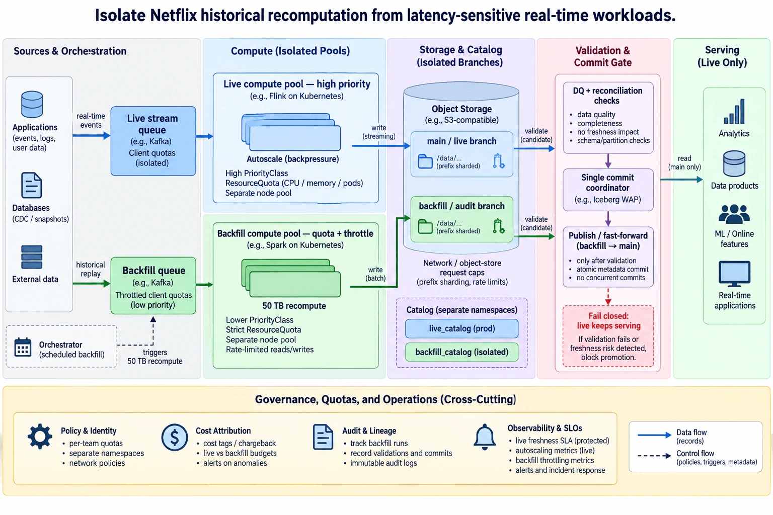
Isolate Netflix historical recomputation from latency-sensitive real-time workloads. diagram
How to Explain It in an Interview
1. Protect the live workload as the primary constraint

The live stream is the protected workload. Applications produce real-time events into a dedicated live stream queue. That queue has isolated client quotas and feeds a high-priority live compute pool. Historical replay does not enter this path. Databases, snapshots, and external historical data feed a separate backfill queue, and the orchestrator triggers the scheduled 50 TB recomputation through that lane.

The main trade-off is deliberate duplication of capacity and operational controls. It can cost more than putting everything in one shared pool, but it creates a much clearer blast-radius boundary around the workload that owns the freshness SLA.

2. Separate queues and compute pools

The live queue feeds the live compute pool, represented in the diagram by streaming processing such as Flink on Kubernetes. The pool has a high PriorityClass, ResourceQuota limits, a separate node pool, and autoscaling driven by live workload pressure such as backpressure. These controls protect CPU, memory, and worker capacity for the ongoing stream.

The backfill queue feeds a different batch compute pool, represented by Spark on Kubernetes. It has a lower PriorityClass, a strict ResourceQuota, a separate node pool, and autoscaling only within its assigned quota. Reads and writes are rate-limited. This means the backfill can scale inside its own boundary but cannot grow without limit or displace the protected live workload.

The queue is also an admission-control boundary. If the backfill pool reaches its quota, historical work waits or slows in its own lane rather than consuming live workers. If live pressure rises, the platform can throttle the backfill without stopping the streaming path.

3. Keep storage writes separate until validation

Both lanes use object storage, but they write through separate logical branches. Streaming writes to the main/live branch. The historical recomputation writes to the backfill/audit branch. This keeps unvalidated historical results away from consumers.

The object store can still be a shared physical resource, so logical branches alone do not provide complete isolation. The platform therefore applies network and object-store request caps to the backfill lane, including rate limits around the shared storage path. The first likely bottleneck during a large recomputation may be shared I/O rather than CPU, so the platform watches live freshness, streaming autoscaling signals, and backfill throttling metrics while the recomputation runs.

4. Isolate metadata visibility with separate catalog namespaces

The main/live branch is registered in the production live catalog namespace. The backfill branch is registered in a separate isolated backfill catalog namespace. The catalog stores metadata about those logical table states; production records remain in object storage in the data plane.

Separate namespaces reduce accidental discovery or use of unvalidated backfill output. They are not the only isolation boundary. Workload identity, per-team quotas, separate compute capacity, network policies, and publication permissions provide the additional controls shown in the platform.

5. Make publication an explicit audit and commit boundary

The two data paths meet only at the validation and commit gate. Before publication, the candidate backfill is checked for data quality, completeness, freshness impact, and schema or partition consistency. Reconciliation is important because successful file generation does not prove that the recomputed business result is correct.

After validation, a single metadata commit coordinator controls publication. The diagram uses an Iceberg-style write-audit-publish boundary: the backfill remains isolated until validation succeeds, and then the backfill branch is fast-forwarded into main through an atomic metadata commit. The publication boundary does not allow concurrent commits during that promotion step.

This makes the merge boundary easy to reason about. Consumers never read a partially validated backfill. They continue reading main, and the validated state becomes consumer-visible only after the publication operation succeeds.

6. Serve only the live/main branch

Analytics, data products, ML or online features, and real-time applications read only from main. They do not read the backfill branch directly. This prevents a partially complete or failed recomputation from becoming consumer-visible.

The important behavioral contract is that historical processing may slow, pause, retry, or fail while the live path continues. A backfill is recomputation. It is not failover, and it does not replace the live stream while it runs.

7. Fail closed when historical results are unsafe

If data-quality checks fail, reconciliation fails, or the platform detects unacceptable freshness impact, the publication gate blocks promotion. The backfill branch remains isolated for inspection or rerun. Live processing continues writing to main and consumers continue reading main.

A failed batch task can be retried inside the backfill lane, but task recovery does not prove that the resulting data is valid. After recovery, the candidate must pass the audit gate again before publication. This separates processing recovery from data correctness.

If metadata publication itself cannot complete safely, the coordinator leaves main as the consumer-visible state. Operators inspect the failed publication, reconcile the candidate against the current live state when needed, and retry through the same controlled commit boundary.

8. Apply governance and identity across both lanes

Policy and identity controls are cross-cutting. Teams receive per-team quotas, separate namespaces, and network policies appropriate to their workloads. The platform records which backfill ran, which validation checks were executed, and which metadata publication occurred.

Audit and lineage tracking records backfill runs, validation results, and commits. Immutable audit logs provide evidence for troubleshooting and make it possible to distinguish a bad historical dataset from a platform-resource failure.

9. Attribute cost to the workload that causes it

Live and backfill workloads receive separate cost tags or chargeback attribution. The platform distinguishes live spend from historical recomputation spend and can alert on cost anomalies. This matters because a 50 TB recomputation can create temporary compute, object-store request, and network costs even when long-term storage growth is not the main bottleneck.

Cost controls should not take resources away from the protected live workload. When the backfill reaches its assigned budget or quota boundary, the safer action is to throttle or pause historical work.

10. Observe the SLA and contention boundaries

The operations layer watches the protected live freshness SLA, live autoscaling signals, and backfill throttling metrics. Alerts and incident response focus first on whether the historical lane is affecting the live lane. If live saturation or freshness risk appears, the immediate containment action is to reduce or stop backfill work.

The platform also keeps audit evidence for backfill executions, validations, and commits. This makes the operating model repeatable instead of depending on manual knowledge for each recomputation.

11. Keep ownership boundaries explicit

Producer and data teams own their event sources, historical source data, recomputation logic, and domain-specific reconciliation rules. The platform team owns the reusable queues, compute isolation, quotas, node-pool boundaries, network policies, catalog separation, commit gate, audit framework, observability, and cost attribution.

The orchestrator schedules the backfill and triggers work into the backfill queue. It does not perform the transformation. Processing engines transform data, object storage keeps records, the catalog keeps metadata, and the commit coordinator controls publication.

The reusable paved road is the isolated backfill lane with standard quotas, audit checks, and publication gates. Exceptional workloads may need different resource limits, but they should not bypass live protection or publish unvalidated data directly into main.

12. Explain the main trade-offs

Dedicated pools and queues reduce resource efficiency because live capacity is protected while backfill capacity is constrained. In return, they make the live blast radius more predictable.

Separate storage and catalog branches add metadata and operational complexity. In return, they keep unvalidated historical state invisible to normal consumers.

Throttling the backfill increases recomputation duration. In return, it protects live latency, network capacity, and object-store request capacity.

A gated metadata publication step adds coordination and can delay availability of the completed backfill. In return, consumers see a controlled main state instead of a partially published historical result.

Technical Approach
  1. Treat the live freshness SLA as the protected objective and identify every resource that the backfill could contend for.
  2. Create separate live and backfill queues so admission control and priority are applied before compute.
  3. Place streaming and historical recomputation in separate compute pools with independent node pools, ResourceQuota limits, PriorityClass settings, and autoscaling boundaries.
  4. Give the backfill lower priority and throttle its object-store reads, writes, and network usage so shared infrastructure cannot be saturated by historical work.
  5. Send live output to the main/live storage branch and historical output to the backfill/audit branch.
  6. Register live and backfill metadata in separate catalog namespaces while keeping production records in object storage.
  7. Run data-quality, completeness, reconciliation, freshness-impact, and schema or partition checks on the backfill candidate.
  8. Route successful candidates through one metadata commit coordinator and allow promotion only after validation and without a concurrent publication commit.
  9. Fast-forward the validated backfill into main through the controlled publication boundary.
  10. Allow analytics, data products, ML or online features, and real-time applications to read main only.
  11. Fail closed on validation or publication problems so the backfill remains isolated while live processing and serving continue.
  12. Track quotas, freshness, throttling, lineage, audit evidence, and cost separately for live and backfill workloads.
Practical Insights

The main scaling problem is not only processing 50 TB. The historical job can also create large bursts of object-store reads, writes, network traffic, metadata operations, and worker demand. The separate backfill pool lets its worker count grow only inside a quota, while the live pool scales according to streaming pressure. If the backfill needs more capacity than allowed, it takes longer instead of borrowing protected live resources. Storage usage temporarily grows while main and backfill branches coexist, and publication adds metadata coordination work. Operational complexity also increases because the platform maintains two queues, two compute pools, separate catalog namespaces, audit gates, and workload-specific monitoring. That extra complexity buys a smaller failure blast radius. Cost is attributed separately so a large recomputation remains visible instead of being mixed into normal live-platform spend. No fixed throughput, completion time, or savings should be promised without measured workload data.

Why Interviewers Ask This

This question tests whether a Data Engineer can protect a latency-sensitive platform from noisy-neighbor effects while still supporting a very large historical recomputation. A strong answer separates compute, queueing, storage, metadata, publication, and operating boundaries instead of treating the backfill as just another batch job. It also tests judgment around quotas, autoscaling, shared network and object-store contention, coordinated metadata publication, cost ownership, audit evidence, and failure isolation.

Common interview mistakes

A common mistake is putting streaming and backfill jobs in the same queue or compute pool and assuming autoscaling alone prevents interference. Autoscaling can increase contention if both workloads compete for the same finite resources. Another mistake is separating compute but ignoring shared network and object-store request pressure. A third is writing backfill output directly into the live branch before reconciliation. Separate catalog namespaces also should not be described as complete workload isolation. Other mistakes include letting consumers read the audit branch, allowing uncontrolled concurrent publication commits, treating a successful batch retry as proof of correctness, or throttling live processing instead of the lower-priority backfill when contention appears.

Interview tip

Start with the invariant: live freshness must survive any backfill failure. Then trace the blue live path and green backfill path separately, explain where they still share infrastructure, and finish at the single validation-and-commit boundary where historical data is allowed to join main. Tie each isolation control to a specific noisy-neighbor risk.
Interviewer may ask next
What would you do if the 50 TB backfill starts increasing live stream lag even though the compute pools are separate?

I would treat that as evidence that the contention is outside the compute boundary. The first suspects are shared network capacity and object-store request pressure. I would use live freshness, streaming backlog or backpressure, and the backfill throttling signals as the protection signals, then reduce the backfill's read and write rate or pause its workers. The backfill remains in its own queue and compute lane, so containment does not stop live processing. I would inspect object-store request pressure, network saturation, and backfill I/O metrics to identify the shared bottleneck. I would not increase backfill capacity until the live workload is healthy. After containment, the historical run can resume in its own lane and must still pass the normal audit gate before publication.

Assume the backfill finishes and passes validation, but a live metadata commit occurs while the backfill is being promoted. How should the platform handle that conflict?

The publication boundary should defer or reject the backfill promotion rather than overwrite a newer main state. The backfill stays in its isolated audit branch while the commit coordinator compares the candidate's expected main state with the current main state. The platform then reconciles the candidate against the newer live state or recomputes the affected merge boundary when required by the data product. Only after reconciliation succeeds does the candidate pass through the validation and commit gate again. Consumers continue reading main throughout the process. This can add publication latency, but it avoids exposing an unsafe merge or losing live updates.

12. Explain how you would simplify and tune a complex SQL query built from several CTEs.PerformanceEasyNetflix

Question Details

Use a reported Netflix analytical query with layered CTEs and first establish the required output grain. Inspect whether each CTE filters, deduplicates, aggregates, or only renames data; check repeated scans, materialization behavior, join cardinality, predicate pushdown, selected columns, and plan estimates. Describe the before-and-after measurements and correctness checks rather than rewriting solely for brevity.

Short Interview Answer (30-60 seconds)

I first define the required output grain, then classify each CTE as filtering, deduplicating, aggregating, or pass-through. I inspect the physical plan for repeated scans, cardinality errors, pushdown, selected columns, and materialization, make the smallest semantics-preserving rewrite, then rerun the same workload and verify identical results.

Detailed Explanation

A complex query with many CTEs is not automatically slow, and making the SQL shorter is not the real objective. I would first define exactly what one output row represents and what duplicate, null, precision, and ordering semantics must be preserved. Then I would classify every CTE by purpose and inspect the actual execution plan and statistics. The important question is whether the layered SQL causes unnecessary physical work such as repeated scans, excessive columns, poor cardinality estimates, missed predicate pushdown, or materialization. I would change only what the evidence supports, rerun the same workload, and validate equivalent results.

Useful Questions to Ask the Interviewer
  1. What is the required final output grain, for example one row per content_id and date?
  2. Which CTEs filter, deduplicate, aggregate, enrich, or only rename/pass data through?
  3. Can I inspect the physical execution plan and actual runtime statistics, not only the SQL text?
  4. Are the same base tables scanned multiple times by different CTEs?
  5. Does this engine inline or materialize these CTEs in this particular plan?
  6. Are estimated join row counts close to actual row counts, or is there a cardinality error or row blowup?
  7. Can we compare the same representative workload before and after the change?
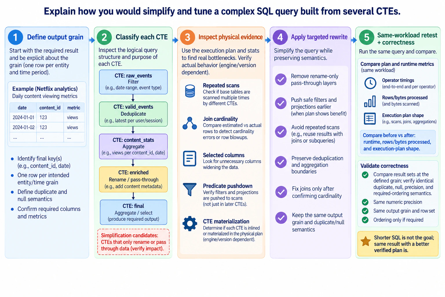
Explain how you would simplify and tune a complex SQL query built from several CTEs. diagram
How to Explain It in an Interview

I would start with the output contract. In the diagram, the analytical result is daily content-viewing metrics, so I first identify the final keys, such as content_id and date, require one row per intended entity/time grain, define duplicate and null behavior, and confirm which columns and metrics are actually needed. This prevents an optimization from silently changing the meaning of the query.

Next, I classify each CTE by its logical purpose. The diagram shows raw_events as a filtering CTE, valid_events as a deduplication CTE, content_stats as an aggregation CTE, enriched as a rename/pass-through simplification candidate, and final as the aggregation/select step that produces the required output. If an apparently pass-through layer actually performs enrichment such as joining metadata, I would treat it according to that real behavior rather than remove it just because its name or SQL looks simple.

Then I inspect physical evidence. I use the execution plan and runtime statistics to look for repeated scans of the same base table, unnecessary selected columns, and join-cardinality problems. For joins, I compare estimated versus actual rows because a large mismatch can indicate poor estimates or unexpected row multiplication. I also verify whether filters and projections actually reach the scan rather than assuming that a logical WHERE clause proves physical predicate or projection pushdown.

I also check how the engine treats each CTE in this specific physical plan. A CTE may be inlined or materialized depending on the engine, version, query shape, and optimizer rules, so I do not assume that CTE syntax itself creates or removes physical work. The physical plan and runtime evidence are what matter.

The rewrite is targeted rather than cosmetic. I remove rename-only or pass-through layers when they add no useful semantic boundary, move safe filters and projections earlier when the resulting physical plan benefits, and reshape repeated work only when the plan demonstrates that the change eliminates unnecessary scans or intermediate processing. I preserve deduplication and aggregation boundaries, and I change joins only after confirming cardinality and duplicate behavior. Throughout the rewrite, I keep the same output grain and the same duplicate and null semantics.

Finally, I rerun the same workload and compare before versus after using runtime, operator timings, rows and bytes processed, bytes scanned when available, and execution-plan shape, including scans, joins, and aggregations. I keep representative data, concurrency, cache conditions, and other relevant test conditions comparable. Then I compare result sets at the defined grain and verify the same row set, duplicate behavior, null semantics, numeric precision, and required ordering. The goal is not shorter SQL; it is the same correct result with a better verified execution plan.

Technical Approach
  1. Define the exact output grain and correctness contract: final keys, one-row-per-entity/time semantics, duplicates, nulls, precision, required ordering, columns, and metrics.
  2. Classify every CTE as filter, deduplication, aggregation, enrichment, or rename/pass-through.
  3. Inspect the physical execution plan and runtime statistics rather than judging the SQL text alone.
  4. Check for repeated base-table scans and unnecessary selected columns.
  5. Compare estimated versus actual join rows to identify cardinality errors or row blowups.
  6. Verify physical predicate and projection pushdown at the scan.
  7. Determine whether each CTE is inlined or materialized in the actual plan; treat this as engine/version dependent.
  8. Apply the smallest semantics-preserving rewrite: remove unnecessary pass-through layers, move safe filters/projections earlier when beneficial, and eliminate repeated physical work only when the plan shows the rewrite does so.
  9. Preserve deduplication and aggregation boundaries, and change joins only after confirming cardinality and duplicate behavior.
  10. Rerun the same representative workload under comparable conditions and compare runtime, operator timings, rows/bytes processed, bytes scanned when available, and plan shape.
  11. Compare result sets at the defined grain and verify identical row-set, duplicate, null, precision, and required-ordering semantics.
Practical Insights

The main cost is the amount of physical work the query causes, not the number of CTE names. Repeated scans can increase storage I/O and data processing. Reading unnecessary columns can increase bytes moved and processed. Bad join cardinality can create much larger intermediate results, increasing CPU, memory, network transfer, sorting, and possibly spill work. Materializing an intermediate result can sometimes prevent recomputation, but it also has write, read, storage, and lifecycle costs; materializing a one-use result can add work. Earlier safe filters and projections can reduce downstream data when the engine actually pushes them to scans. Removing a pass-through CTE may improve readability without improving runtime if the optimizer already produces the same physical plan. That is why the same workload must be measured before and after rather than assuming shorter SQL is faster. Maintenance often improves when redundant layers are removed, but meaningful deduplication, enrichment, and aggregation boundaries must remain when they protect correctness.

Why Interviewers Ask This

Interviewers want to see whether you optimize SQL from evidence rather than from appearance. A strong answer establishes the required output grain, understands what every CTE actually does, separates logical SQL structure from the physical execution plan, finds repeated scans or join-cardinality problems, verifies pushdown and CTE materialization behavior, makes only semantics-preserving changes, and proves the result with comparable before-and-after measurements and output-equivalence checks.

Common interview mistakes

Common mistakes are rewriting CTEs only to make the SQL shorter; assuming every CTE is physically materialized; assuming a logical WHERE clause proves predicate pushdown; removing a deduplication, enrichment, or aggregation boundary without checking the resulting grain; using SELECT * and carrying unused columns through the plan; ignoring repeated scans; assuming a subquery or rewritten CTE automatically eliminates a repeated scan without checking the physical plan; changing a join before checking estimated versus actual cardinality and duplicate behavior; trusting plan estimates without comparing actual rows when available; reporting an improvement from a different workload or cache state; inventing benchmark numbers; and declaring success without comparing result sets, null behavior, precision, duplicates, and required ordering.

Interview tip

Present this as an evidence-driven sequence: define the output grain, classify the CTEs, inspect the physical plan, identify one real source of unnecessary work, make the smallest semantics-preserving change, rerun the same workload, and prove output equivalence. Emphasize that shorter SQL is not the goal; a measurably better verified plan with the same result is.

Interviewer may ask next
Would you always remove a CTE that only renames columns or passes rows through?

No. I would treat it as a simplification candidate, not automatically delete it. First I would confirm what it really does and inspect the physical plan. If removing it preserves the same output contract and either improves the plan or leaves the plan unchanged while making the query easier to maintain, I would simplify it. If it performs real enrichment, creates a useful semantic boundary, or its treatment changes materialization or reuse in the specific engine and plan, I would keep it.

How would you prove that the tuned query is actually better and still correct?

I would rerun the same representative workload under comparable conditions and compare execution-plan shape, operator timings, runtime, rows and bytes processed, and bytes scanned when available. Then I would compare the original and tuned result sets at the defined output grain and verify the same rows, duplicate behavior, null semantics, numeric precision, and required ordering. I would not claim an optimization merely because the rewritten SQL is shorter.

13. Implement a streaming word counter with query operations.CodingEasyNetflix

Question Details

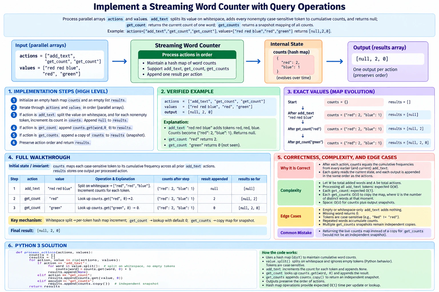
Process parallel arrays actions and values. add_text splits its value on whitespace, adds every nonempty case-sensitive token to cumulative counts, and returns null; get_count returns the current count of one word; get_counts returns a snapshot mapping of all counts. Support at most 10,000 actions and 100,000 total words. Example: actions=["add_text","get_count","get_count"], values=["red red blue","red","green"] returns [null,2,0].

Short Interview Answer (30-60 seconds)

I would keep one hash map from each case-sensitive word to its cumulative count and process the actions in order. For add_text, I split the value on whitespace and increment every token. For get_count, I return the stored count or 0. For get_counts, I return a copy so later updates cannot change an earlier snapshot. Processing added words takes O(W) expected time, get_count is O(1) expected time, and each snapshot costs O(U). The live map uses O(U) space.

Detailed Explanation

See the Code while reading this explanation.

The input contains two parallel arrays named actions and values. Items at the same position belong together, and we process them from left to right. add_text splits its text on whitespace and adds every nonempty case-sensitive word to running counts. get_count returns the current count of one word, or 0 when it has not appeared. get_counts returns a snapshot copy of all current counts. We return one result per action in the same order. add_text returns null. The solution supports up to 10,000 actions and 100,000 total added words.

Useful Questions to Ask the Interviewer
  1. Should words remain case-sensitive exactly as given? The stated contract says yes.
  2. Should get_counts return an independent snapshot instead of the live map? The stated contract says yes.
  3. Can I assume actions and values are parallel arrays with matching positions?
Implement a streaming word counter with query operations. diagram
How to Explain It in an Interview
1. Understand the input and required output

I receive actions and values as parallel arrays. I process actions[i] together with values[i]. I build a results list with exactly one result for every action. add_text produces null. get_count produces one integer. get_counts produces a snapshot mapping of all current counts.

2. Choose the data structure

I use a hash map named counts. Each key is one case-sensitive word. Its value is that word's cumulative frequency across all add_text operations processed so far. A hash map fits because updating or reading one word is O(1) on average.

3. Initialize and process actions in order

I start with counts = {} and results = []. I then walk through actions and values together in order. For add_text, value.split() separates the text on whitespace and does not produce empty tokens. I increment every token and append None. For get_count, I append counts.get(value, 0). For get_counts, I append counts.copy() so the returned snapshot is independent of later updates.

4. Walk through the example

The example uses actions = ["add_text", "get_count", "get_count"] and values = ["red red blue", "red", "green"]. First, add_text processes "red red blue". The tokens are "red", "red", and "blue". counts changes from {} to {"red": 2, "blue": 1}, and results changes from [] to [null]. Next, get_count("red") reads 2. counts stays {"red": 2, "blue": 1}, and results becomes [null, 2]. Finally, get_count("green") does not find the word, so it returns 0. counts stays {"red": 2, "blue": 1}, and the final result is [null, 2, 0].

5. Explain why the result is correct

After every processed action, counts stores the cumulative frequency of every case-sensitive word added by all add_text actions seen so far. Query operations do not change this state. Because actions are processed in order and exactly one output is appended for each action, the result positions stay aligned with the input actions. Using a copy for get_counts also keeps each returned snapshot independent from future updates.

6. Explain the Python implementation

The function creates the counts map and results list. It uses zip(actions, values) to process each action with its matching value. add_text calls value.split() and increments counts with counts.get(word, 0) + 1. get_count uses counts.get(value, 0). get_counts uses counts.copy(). The function then returns results in action order.

7. Explain complexity and edge cases

Let W be the total number of words processed by add_text and U be the number of distinct words currently stored. Processing all add_text tokens takes O(W) expected time because dictionary lookup and insertion are O(1) on average. Each get_count is O(1) expected time. Each get_counts is O(U) because it copies the whole map. The live counts map uses O(U) extra space, plus the space needed by returned snapshots. Empty or whitespace-only text adds nothing. Missing words return 0. Repeated words accumulate. Case variants such as "Red" and "red" are separate keys.

Key Insight / Why This Solution Works

The key idea is to maintain one cumulative hash map instead of recomputing frequencies for every query. The invariant is: after each processed action, counts maps every case-sensitive word seen in all processed add_text operations to its cumulative frequency. add_text updates this state. get_count reads one value without changing it. get_counts copies the current state. This directly matches the diagram's single-pass action flow and supports the stated limits efficiently.

Code
def process_actions(actions: list[str], values: list[str]) -> list[object]:
    # Store the cumulative count for each case-sensitive word.
    counts: dict[str, int] = {}

    # Keep exactly one output for every processed action.
    results: list[object] = []

    # Process each action together with the value at the same position.
    for action, value in zip(actions, values):
        if action == "add_text":
            # Split on whitespace; Python does not return empty tokens here.
            for word in value.split():
                # Increment the existing frequency, or start a new word at 1.
                counts[word] = counts.get(word, 0) + 1

            # add_text changes state but returns no value.
            results.append(None)

        elif action == "get_count":
            # Return the current count, using 0 when the word has not appeared.
            results.append(counts.get(value, 0))

        elif action == "get_counts":
            # Copy the map so later updates cannot change this snapshot.
            results.append(counts.copy())

    # Return outputs in the same order as the input actions.
    return results


def main() -> None:
    # Run the exact example shown in the approved diagram.
    actions = ["add_text", "get_count", "get_count"]
    values = ["red red blue", "red", "green"]

    # Python prints [None, 2, 0], equivalent to JSON [null, 2, 0].
    print(process_actions(actions, values))


if __name__ == "__main__":
    main()
Time & Space Complexity

Let W be the total number of words added by all add_text operations and U be the number of distinct words currently stored. Python dictionary lookup and insertion are O(1) on average, so processing all added tokens takes O(W) expected time. Each get_count takes O(1) expected time. Each get_counts takes O(U) because it copies every current entry. The live counts dictionary uses O(U) extra space. Returned snapshots use additional output space proportional to the maps that were copied.

Where it is used

This pattern is useful when software receives updates over time and must answer queries from the current accumulated state. Examples include counting words in incoming text batches, maintaining event frequencies, tracking category counts in a data pipeline, and exposing current statistics while new records continue to arrive.

Why Interviewers Ask This

This problem checks whether you can maintain state while processing ordered operations. The interviewer can see whether you choose a suitable hash map, preserve cumulative counts, handle repeated and missing words, keep case sensitivity correct, and return snapshots safely. It also tests whether you understand the difference between reading shared state and copying it, and whether you can describe expected hash-map complexity accurately.

Common interview mistakes

A common mistake is replacing the counts map on each add_text instead of keeping cumulative counts. Another is lowercasing tokens even though the contract is case-sensitive. Candidates may return an error for a missing word instead of 0. For get_counts, returning the live counts dictionary is also wrong because later updates would change an earlier snapshot. Another mistake is using splitting logic that creates empty tokens. Finally, candidates may forget that copying the map makes each get_counts operation O(U).

Interview tip

State the invariant early: counts always represents all words added so far. Then describe each operation as one of three things: update that state, read one count, or copy the state for a snapshot. This makes both the code and the correctness argument easy to explain.

Interviewer may ask next
What changes if get_counts is called very often and copying the whole map becomes expensive?

In the current design, each get_counts call copies U distinct entries, so it costs O(U) time and O(U) output space. If the contract still requires an independent ordinary mapping, that copy is required by this implementation. A different API could return a read-only view or use a persistent data structure, but that would change the representation or snapshot design. add_text and get_count can still keep their current expected-time behavior.

How does the solution handle many separate add_text operations containing the same word?

No algorithm change is needed. Every add_text operation reads the current value with counts.get(word, 0) and increments it. The count therefore remains cumulative across all operations. If the same word appears k additional times, its stored count increases by k. Processing those k tokens takes O(k) expected time, and the live map still uses O(U) space for U distinct words.

14. Find the maximum overlap of closed intervals and the overlap count at each query point.CodingMediumNetflix

Question Details

Implement closed_interval_overlap(intervals, query_points). Each interval [start,end] is closed and may be repeated, nested, unsorted, or reduced to one point; coordinates are signed integers. Return [[maximumOverlap], queryCounts], where queryCounts aligns with the original query order and empty intervals give maximumOverlap 0. Support up to 200,000 intervals and query points. Example: intervals=[[1,3],[3,5],[3,3]], queries=[0,3,4] returns [[3],[0,3,1]].

Short Interview Answer (30-60 seconds)

I would separate all interval starts and ends, sort both lists, and use a two-pointer sweep to find the maximum overlap. Because the intervals are closed, I process a start before an equal end, so intervals touching at the same coordinate still overlap. For each query point, I use binary search to count starts at or before it minus ends before it. The total time is O(n log n + q log n), with O(n) auxiliary space plus the returned query-count list.

Detailed Explanation

See the Code while reading this explanation.

We receive closed intervals and query points. We need two results. First, we need the largest number of intervals that cover the same coordinate. Second, we need the number of intervals covering each query point, in the original query order. I separate the starts and ends and sort them. A sweep over these sorted values finds the largest overlap. Binary searches answer each query. The important detail is that an interval includes both endpoints, so a start at a coordinate must be counted before an end at that same coordinate.

Useful Questions to Ask the Interviewer
  1. Should I treat both interval endpoints as inclusive? Here the answer is yes because every interval is closed.
  2. Should the query counts stay in the same order as the input query points? Here the answer is yes.
  3. Can intervals be repeated, nested, unsorted, or single points? The problem says all of these are allowed.
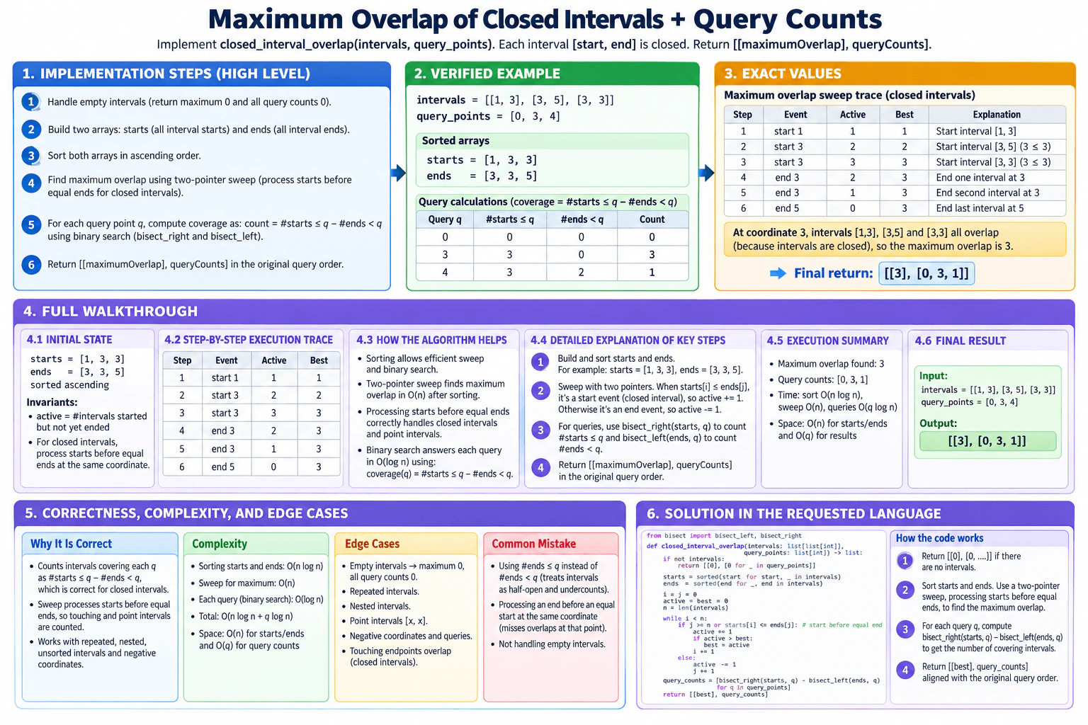
Find the maximum overlap of closed intervals and the overlap count at each query point. diagram
How to Explain It in an Interview
1. Understand the input and required output

The input contains intervals and query_points. Each interval is [start, end] and includes both endpoints. The function returns [[maximumOverlap], queryCounts]. queryCounts[i] is the number of intervals containing query_points[i]. If there are no intervals, the maximum overlap is 0 and every query count is 0.

For the example, the intervals are [[1,3],[3,5],[3,3]] and the query points are [0,3,4]. The required result is [[3],[0,3,1]].

2. Build and sort the endpoint arrays

I create one list containing every start and another list containing every end. For the example, the sorted starts are [1,3,3] and the sorted ends are [3,3,5].

Sorting lets us process interval events in coordinate order. It also lets us answer each query with binary search.

3. Sweep the endpoints to find the maximum overlap

I keep two indices, one for starts and one for ends. I also keep active, the number of intervals that have started but have not ended yet, and best, the largest value of active seen so far.

While either endpoint list still has an unprocessed event, I choose the next event. If a start exists and it is less than or equal to the next end, I process the start first. I increase active, update best, and advance the start index. Otherwise, I process an end, decrease active, and advance the end index.

The <= comparison is essential because these intervals are closed. At coordinate 3 in the example, all three intervals [1,3], [3,5], and [3,3] contain 3. Processing the two starts at 3 before the ends at 3 lets active reach 3.

The sweep is: 1. Start at 1: active becomes 1 and best becomes 1. 2. Start at 3: active becomes 2 and best becomes 2. 3. Start at 3: active becomes 3 and best becomes 3. 4. End at 3: active becomes 2 and best stays 3. 5. End at 3: active becomes 1 and best stays 3. 6. End at 5: active becomes 0 and best stays 3.

So the maximum overlap is 3.

4. Answer every query with binary search

For a query point q, an interval contains q when its start is at or before q and its end is at or after q.

bisect_right(starts, q) gives the number of interval starts <= q. bisect_left(ends, q) gives the number of interval ends < q. Therefore the number of intervals covering q is:

bisect_right(starts, q) - bisect_left(ends, q)

For q = 0, the count is 0 - 0 = 0. For q = 3, it is 3 - 0 = 3. For q = 4, it is 3 - 2 = 1. This produces [0,3,1] in the original query order.

5. Explain why the result is correct

During the endpoint sweep, active represents intervals that have started but whose end event has not yet been processed. Processing a start before an equal end preserves closed-interval behavior, so intervals sharing an endpoint are simultaneously active there.

For a query, the formula counts all intervals that have started by q and subtracts only intervals that ended strictly before q. Intervals ending exactly at q remain counted because the endpoints are inclusive.

6. Explain complexity and edge cases

Sorting the two endpoint lists costs O(n log n). The two-pointer sweep processes 2n endpoint events in O(n) time. Each query uses two binary searches and costs O(log n), so q queries cost O(q log n). Total time is O(n log n + q log n).

The sorted start and end arrays use O(n) auxiliary space. The returned query-count list contains O(q) values. Important cases include empty intervals, repeated intervals, nested intervals, point intervals such as [3,3], negative coordinates, and intervals that only touch at an endpoint.

Key Insight / Why This Solution Works

The key idea is to represent every interval with two sorted endpoint arrays. The maximum-overlap part uses a two-pointer sweep. Its invariant is that active equals the number of intervals that have started but whose end event has not yet been processed. For closed intervals, a start at coordinate x must be processed before an end at x, which is why the comparison uses starts[i] <= ends[j] when both events exist. The sweep continues until both endpoint lists are exhausted. Query counts use the same sorted arrays. For a query q, the answer is the number of starts <= q minus the number of ends < q. This correctly keeps intervals ending exactly at q in the count.

Code
from bisect import bisect_left, bisect_right


def closed_interval_overlap(intervals: list[list[int]], query_points: list[int]) -> list[list[int]]:
    # With no intervals, the maximum overlap is 0 and no query is covered.
    if not intervals:
        return [[0], [0 for _ in query_points]]

    # Sort interval starts and ends separately so endpoint events can be swept
    # in order and the same arrays can answer point queries by binary search.
    starts = sorted(start for start, _ in intervals)
    ends = sorted(end for _, end in intervals)

    # active is the number of intervals currently covering the sweep position.
    # best is the largest active count seen so far.
    n = len(intervals)
    i = 0
    j = 0
    active = 0
    best = 0

    # Sweep all 2n endpoint events. For closed intervals, process a start at x
    # before an end at the same x so both intervals are counted at coordinate x.
    while i < n or j < n:
        if i < n and (j >= n or starts[i] <= ends[j]):
            active += 1
            if active > best:
                best = active
            i += 1
        else:
            # The next event is an end, so that interval stops being active
            # after its closed endpoint has been counted at this coordinate.
            active -= 1
            j += 1

    # For each q, count starts <= q and subtract only ends < q.
    # An interval ending exactly at q remains included because it is closed.
    query_counts = []
    for q in query_points:
        count = bisect_right(starts, q) - bisect_left(ends, q)
        query_counts.append(count)

    # Keep the maximum in its required one-element list and preserve query order.
    return [[best], query_counts]


def main() -> None:
    # Run the exact example used in the approved diagram.
    intervals = [[1, 3], [3, 5], [3, 3]]
    query_points = [0, 3, 4]
    result = closed_interval_overlap(intervals, query_points)
    print(result)


if __name__ == "__main__":
    main()
Time & Space Complexity

Let n be the number of intervals and q be the number of query points. Sorting the starts and ends takes O(n log n) time. The two-pointer sweep processes 2n endpoint events, which is O(n) time. Each query performs two binary searches, so each query takes O(log n), and all queries take O(q log n). The total time is O(n log n + q log n). The two sorted endpoint arrays require O(n) auxiliary space. The returned query-count list contains O(q) output values.

Where it is used

This pattern is useful when software needs to measure how many time ranges, reservations, sessions, jobs, or validity windows are active at particular points. Separating and sorting endpoints is especially useful when many point queries must be answered without scanning every interval for every query.

Why Interviewers Ask This

This question tests whether a candidate can turn interval boundaries into ordered events, handle inclusive endpoints correctly, and reuse sorted data for many queries. It also checks two-pointer reasoning, binary-search boundary choices, duplicate and point-interval handling, and complexity analysis. The important detail is not just sorting. The candidate must explain why equal starts come before equal ends and why query counting uses <= q for starts but < q for ends.

Common interview mistakes

A common mistake is processing an end before a start when both have the same coordinate. That incorrectly treats closed intervals as half-open and can reduce the maximum overlap. Another mistake is subtracting ends <= q when answering a query. The correct subtraction is ends < q, because an interval ending exactly at q still contains q. Candidates may also forget the empty-input case, lose the original query order, stop the sweep before matching the illustrated full endpoint trace, or scan every interval for every query and create O(nq) work.

Interview tip

State the closed-interval rule before writing the sweep: when a start and end have the same coordinate, process the start first. Then connect the same rule to the query formula: count starts <= q, but subtract only ends < q. This makes the endpoint semantics easy to verify in both parts of the solution.

Interviewer may ask next
Why would the answer be wrong if we processed an end before a start at the same coordinate?

The intervals are closed, so both endpoints belong to the interval. If one interval ends at x and another starts at x, both cover x. Processing the end first would remove the first interval before adding the second one and could miss the true overlap at x. Processing starts first makes all intervals containing that coordinate active together. The algorithm still takes O(n log n + q log n) time and O(n) auxiliary space, plus the O(q) returned result.

What changes if many query points contain the same value?

The current code is still correct because every query independently uses the same two binary searches and keeps the original query order. If repeated query values are common, we can cache the count for each distinct query value and reuse it. If there are u distinct query values, the query work becomes O(u log n + q) instead of O(q log n). The total time becomes O(n log n + u log n + q), and the cache adds O(u) memory on top of the O(n) endpoint arrays and O(q) returned result.

15. Produce exactly-once daily event counts from two-hour-late, duplicated member events.CodingHardNetflix

Question Details

Implement daily_event_counts(events). Each record is (member_id,event_name,ts_ms,payload_json), delivery may be out of order by up to two hours, and the logical identity is the complete four-field tuple. Deduplicate that identity, use event time to assign a UTC day, and emit one count per (day,event_name,member_id) only after the two-hour watermark makes the day final; replaying the same input must not change output. Example: two identical PLAY rows for m1 at day-1 10:00 plus one distinct PLAY row at 10:01 produce count 2 for that day and member.

Short Interview Answer (30-60 seconds)

I would use event time, a set for full-record deduplication, and a count map keyed by UTC day, event name, and member. For each event, I first check the complete four-field tuple. Only a new tuple increments its count. I keep this state checkpointed and wait for a two-hour event-time watermark to pass the day's end before emitting the final count. With average O(1) hash operations, processing is O(n) expected time and uses O(u + k) active state.

Detailed Explanation

See the Code while reading this explanation.

Each record contains a member ID, an event name, a timestamp, and a JSON payload. Records may arrive in the wrong order by up to two hours, and the same complete record may arrive more than once. We must count each distinct four-field record once. The timestamp decides the UTC day. We publish one final count for each (day, event_name, member_id) only after the watermark has passed that day's end. Replaying the same committed input must not change the output.

Useful Questions to Ask the Interviewer
  1. Should payload_json be compared exactly as supplied when building the four-field deduplication identity?
  2. Can I treat events that arrive behind the finalized watermark as outside the stated two-hour lateness guarantee?
  3. Does the output support an exactly-once transaction or an idempotent upsert keyed by (day, event_name, member_id)?
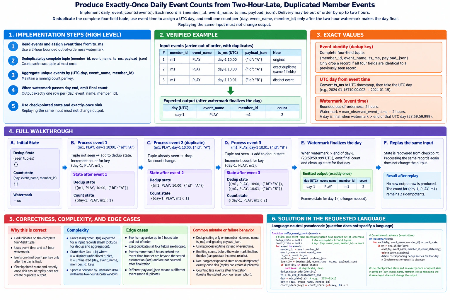
Produce exactly-once daily event counts from two-hour-late, duplicated member events. diagram
How to Explain It in an Interview
1. Understand the input and output

The input record is (member_id, event_name, ts_ms, payload_json). Its logical identity is the complete four-field tuple. The required output grain is one row per (UTC day, event_name, member_id). A result is not final just because the event has been processed. It becomes final only when the two-hour event-time watermark has moved past the end of that UTC day.

2. Initialize the two pieces of state

I keep dedup_state as a hash set of complete event tuples. I also keep count_state as a hash map from (day, event_name, member_id) to the running count. Both are checkpointed. The main invariant is that count_state contains exactly one increment for every unique four-field event identity accepted for that aggregation key.

3. Deduplicate before counting

For every delivered event, I build identity = (member_id, event_name, ts_ms, payload_json). If the identity is already in dedup_state, I drop the event and do not change the count. Otherwise, I add the identity to the set. This prevents an exact retry from contributing twice.

4. Assign the UTC day and aggregate

For a new event, I convert ts_ms to its UTC calendar day. I then build key = (day, event_name, member_id) and increment count_state[key] by one. Arrival order does not choose the day. Event time does.

5. Walk through the verified example

The first event is (m1, PLAY, day-1 10:00, {"id":"A"}). It is new, so the deduplication set stores it and the count for (day-1, PLAY, m1) becomes 1. The second row is identical in all four fields. It is dropped, so the count stays 1. The third event is (m1, PLAY, day-1 10:01, {"id":"B"}). Its timestamp and payload make it a different identity, so the count becomes 2.

6. Finalize with the two-hour watermark

The diagram uses watermark = maximum observed event time minus two hours. While the watermark is still inside day-1, its count is not final. When the watermark moves past the end of day-1 at 23:59:59.999 UTC, I emit (day-1, PLAY, m1, 2). After the final output is safely committed, the per-day count and deduplication state for that finalized day can be removed.

7. Make replay safe and explain complexity

The processing state is checkpointed, and the sink must participate in exactly-once delivery or use an idempotent upsert at the output grain. That keeps a recovery or replay from creating another logical result. With hash-based state, each input record needs expected O(1) set and map operations, so n records take O(n) expected time. Active state is O(u + k), where u is the number of distinct unfinalized identities and k is the number of unfinalized count keys.

Key Insight / Why This Solution Works

Use three ordered stages. First, deduplicate using the exact four-field tuple (member_id, event_name, ts_ms, payload_json). Second, assign each accepted event to a UTC day using ts_ms and increment a hash-map count keyed by (day, event_name, member_id). Third, wait until the two-hour event-time watermark moves past that day's end before emitting its final count. The invariant is that every active count equals the number of distinct accepted identities for that key. Checkpointed state plus an exactly-once or idempotent sink makes recovery and replay safe.

Code
from __future__ import annotations

from dataclasses import dataclass, field
from datetime import datetime, timedelta, timezone
from typing import Iterable, TypeAlias

Event: TypeAlias = tuple[str, str, int, str]
EventIdentity: TypeAlias = tuple[str, str, int, str]
CountKey: TypeAlias = tuple[str, str, str]
OutputRow: TypeAlias = tuple[str, str, str, int]

TWO_HOURS_MS = 2 * 60 * 60 * 1000


def utc_day(ts_ms: int) -> str:
    # Event time, not arrival time, determines the UTC calendar day.
    return datetime.fromtimestamp(ts_ms / 1000, tz=timezone.utc).date().isoformat()


def utc_day_end_ms(day: str) -> int:
    # The last millisecond of the UTC day is the finalization boundary.
    start = datetime.fromisoformat(day).replace(tzinfo=timezone.utc)
    next_day = start + timedelta(days=1)
    return int(next_day.timestamp() * 1000) - 1


@dataclass
class DailyEventCounter:
    # These two structures represent checkpointed processing state.
    dedup_state: set[EventIdentity] = field(default_factory=set)
    count_state: dict[CountKey, int] = field(default_factory=dict)

    # The stream runtime advances this event-time frontier monotonically.
    watermark_ms: int = -1

    # This models an idempotent upsert sink at the exact output grain.
    output: dict[CountKey, int] = field(default_factory=dict)

    def process_event(self, event: Event) -> None:
        member_id, event_name, ts_ms, payload_json = event

        # An event behind the finalized watermark is outside the stated
        # two-hour lateness contract and must not change finalized output.
        if ts_ms <= self.watermark_ms:
            return

        identity: EventIdentity = (
            member_id,
            event_name,
            ts_ms,
            payload_json,
        )

        # Deduplicate on all four fields before performing any aggregation.
        if identity in self.dedup_state:
            return
        self.dedup_state.add(identity)

        # Assign the unique event to its event-time UTC day.
        day = utc_day(ts_ms)
        key: CountKey = (day, event_name, member_id)

        # Each unique identity contributes exactly one increment to its key.
        self.count_state[key] = self.count_state.get(key, 0) + 1

    def advance_watermark(self, new_watermark_ms: int) -> list[OutputRow]:
        # Watermarks only move forward. A repeated or older watermark changes nothing.
        if new_watermark_ms <= self.watermark_ms:
            return []

        self.watermark_ms = new_watermark_ms
        emitted: list[OutputRow] = []

        # Only days whose end is strictly behind the watermark are final.
        final_keys = [key for key in self.count_state if utc_day_end_ms(key[0]) < self.watermark_ms]

        for key in sorted(final_keys):
            count = self.count_state[key]

            # Upsert by output grain so a retry cannot create a second logical row.
            self.output[key] = count
            emitted.append((key[0], key[1], key[2], count))

            # The aggregate is no longer needed after final output is committed.
            del self.count_state[key]

        # Deduplication entries for finalized days can now be removed safely.
        self.dedup_state = {
            identity
            for identity in self.dedup_state
            if utc_day_end_ms(utc_day(identity[2])) >= self.watermark_ms
        }

        return emitted


def daily_event_counts(events: Iterable[Event]) -> DailyEventCounter:
    # Normal event delivery and watermark delivery are separate in a stream runtime.
    counter = DailyEventCounter()
    for event in events:
        counter.process_event(event)
    return counter


def main() -> None:
    day1_1000 = int(datetime(2024, 1, 1, 10, 0, tzinfo=timezone.utc).timestamp() * 1000)
    day1_1001 = int(datetime(2024, 1, 1, 10, 1, tzinfo=timezone.utc).timestamp() * 1000)

    # This is the same example shown in the approved diagram.
    events: list[Event] = [
        ("m1", "PLAY", day1_1000, '{"id":"A"}'),
        ("m1", "PLAY", day1_1000, '{"id":"A"}'),
        ("m1", "PLAY", day1_1001, '{"id":"B"}'),
    ]

    counter = daily_event_counts(events)

    # The stream runtime eventually advances the two-hour event-time watermark
    # past the end of day-1. Only then is the daily result final.
    watermark_after_day1 = int(datetime(2024, 1, 2, 0, 0, tzinfo=timezone.utc).timestamp() * 1000)
    rows = counter.advance_watermark(watermark_after_day1)

    print(rows)
    # [('2024-01-01', 'PLAY', 'm1', 2)]

    # Replaying these already-finalized records is ignored because their event
    # timestamps are behind the finalized watermark, so output stays unchanged.
    for event in events:
        counter.process_event(event)
    counter.advance_watermark(watermark_after_day1)

    print(counter.output)
    # {('2024-01-01', 'PLAY', 'm1'): 2}


if __name__ == "__main__":
    main()
Time & Space Complexity

Let n be the number of delivered records, u the number of distinct event identities still needed for unfinalized days, and k the number of active (day, event_name, member_id) count keys. Python set membership and insertion and dictionary lookup and update are O(1) on average. Therefore processing n records is O(n) expected time. The extra active state is O(u + k). Finalized-day state is removed after its output is safely committed.

Where it is used

This pattern is common in streaming analytics where producers retry records and network delays change arrival order. Examples include playback events, click streams, telemetry, billing records, and operational metrics. Full-identity deduplication prevents retry inflation, event-time grouping puts late records into the correct window, and watermark finalization prevents publishing a daily result too early.

Why Interviewers Ask This

This problem tests practical stream-processing reasoning. The interviewer wants to see whether you distinguish event time from arrival time, define the exact deduplication identity, choose the correct aggregation grain, and understand why a watermark controls final output. It also tests whether you can reason about checkpointed state, replay safety, state cleanup, hash-based complexity, and the difference between processing exactly once internally and producing exactly-once results at the sink.

Common interview mistakes

Deduplicating only (member_id, event_name, ts_ms) is wrong because payload_json is part of the logical identity. Using processing time instead of ts_ms can place a late event into the wrong UTC day. Counting before checking dedup_state inflates the result when retries arrive. Emitting before the watermark passes the day's end can miss valid late data. Another mistake is deleting state before the final output is safely committed or using a sink that can create a second row during replay.

Interview tip

Explain the solution in this order: full four-field identity, UTC event-time aggregation key, then watermark finalization. State exactly what the set and map store. That makes the duplicate example and the final count of 2 easy to verify step by step.

Interviewer may ask next
What changes if events may arrive more than two hours late?

Increase the watermark delay if those events must still be included before finalization. The deduplication and counting logic stays the same, but state must be kept longer and final output is delayed. Processing remains O(n) expected time, while active O(u + k) state can grow because more events and keys remain unfinalized. If already-finalized results must accept later corrections, use deterministic upserts for revised counts instead of treating the first result as immutable.

How would you scale this for a very large stream?

Partition processing so all events for an aggregation key reach the same logical keyed state, and keep deduplication and count state in a durable state backend with checkpoints. Write finalized rows through an exactly-once transaction or an idempotent upsert sink. The algorithm still uses O(n) expected processing time overall and O(u + k) active state, but that state is distributed across workers. The main tradeoff is larger checkpoint and state-management cost as the amount of unfinalized data grows.

Disclaimer: This interview guide is for educational and informational purposes only. It is designed to help readers prepare, but it does not guarantee any interview result, hiring decision, offer, or outcome. Interview questions, hiring criteria, and preferred answers can vary by employer, interviewer, industry, location, and time. The examples and explanations reflect the authors' research and judgment, are provided without warranties of any kind, and should not be treated as the only correct approach. Diagrams are simplified illustrations intended to highlight the main components and their interactions; actual systems and implementations may be more complex. Alternative approaches may be equally valid or better suited to a particular question, context, or interviewer. To the fullest extent permitted by applicable law, the author, contributors, and publisher are not liable for decisions made, actions taken, or losses incurred based on this guide.

Company Notice: This guide is an independent educational resource and is not affiliated with, endorsed by, sponsored by, or approved by the company named in this guide. Company names are used only to identify interview experiences commonly reported by candidates. Interview practices can change without notice, and inclusion of company-specific content does not mean these questions are official, complete, or guaranteed to be asked. To the fullest extent permitted by law, the author, contributors, and publisher are not responsible for outcomes related to use of this material.

Content Accuracy and Verification: To the fullest extent permitted by applicable law, we do not represent or warrant that interview guides, questions, answers, examples, or diagrams are accurate, complete, current, error-free, or suitable for any particular purpose. You are responsible for independently reviewing and verifying the information before relying on it.