Google Data Engineer Interview Questions & Answers

BigQuery separates distributed columnar storage from massively parallel compute slots. Metadata-driven pruning reduces scans, while staged execution, local aggregation, shuffle, and global aggregation spread work across slots. The main trade-off is elastic independent scaling versus managing compute capacity and storage costs separately.

BigQuery serves analysts, data engineers, and applications that need to run analytical SQL over very large datasets without managing database servers. One machine cannot efficiently scan, redistribute, and aggregate petabyte-scale data while also supporting many concurrent queries. BigQuery addresses this by separating a metadata and planning control plane from distributed columnar storage and an independent compute layer made of slots. The design prioritizes reducing data before processing, parallel execution, efficient network exchange, concurrency, task recovery, caching, and independent storage and compute economics rather than relying on one large database node.

1. Are we mainly discussing interactive analytics, scheduled analytical queries, or both?
2. Is the workload using on-demand query pricing, capacity-based reservations, or a mix?
3. Are the largest tables partitioned and clustered so partition and block pruning can reduce scans?
4. Is the main concern single-query latency, high query concurrency, cost control, or a combination of them?
5. Do large joins or aggregations regularly create enough intermediate data to pressure the shuffle layer?

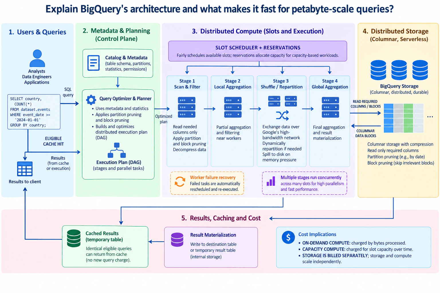
Analysts, data engineers, and applications submit SQL to BigQuery. The example query groups event rows by country and filters on a date. The user does not select machines or attach the data to a fixed compute cluster. BigQuery accepts the query and handles planning, scheduling, distributed execution, storage access, result creation, and delivery as managed platform capabilities.

The important architectural decision is the separation of storage from compute. Table data remains in distributed BigQuery storage while query compute is scheduled independently. That lets storage and compute scale on different boundaries, but it also means their usage and costs must be considered separately.

The query first reaches the metadata and planning control plane. The catalog and metadata layer holds information such as table schema, partitions, statistics, and permissions. The query optimizer and planner use that information to parse and optimize the query and create a distributed execution plan represented as a DAG, or directed acyclic graph, containing stages and parallel tasks.

This control-plane work does not carry the table's production rows. Its purpose is to decide what work the data plane must perform and to reduce unnecessary work before execution starts.

The planner applies partition and block pruning when the table layout and query predicates allow it. A qualifying filter on a partitioning column lets BigQuery skip partitions that cannot contribute rows. Block pruning similarly skips irrelevant storage blocks when block metadata can rule them out.

These optimizations matter twice. They reduce how much data workers must read, and they reduce downstream processing and network work. Under on-demand pricing, reducing the bytes processed also directly reduces query compute cost.

Stage 1 is the scan-and-filter stage. BigQuery storage is shown as distributed, durable, columnar storage with compression. The workers request the required columns and relevant blocks instead of reading complete rows from every part of the table.

Columnar storage is especially effective for analytical SQL because queries commonly reference a small subset of columns from wide tables. Compression reduces the physical data that must be read and moved. Partition pruning and block pruning reduce the storage range even further before decompression and filtering occur in the execution stage.

The optimized plan goes to the distributed compute layer. BigQuery divides work into execution stages, and available slots execute work units in parallel. The diagram shows separate stages for scan and filter, local aggregation, shuffle and repartition, and global aggregation.

The slot scheduler distributes available compute across concurrent work. Many stages and tasks can make progress across many slots, which provides high parallelism without requiring the user to provision individual workers. The practical scaling limit is therefore not one machine but the available compute and the dependencies between stages.

The scheduler and reservation layer are related but not identical concepts. Scheduling applies available slots to query work, while reservations allocate capacity for capacity-based workloads. Reservations give administrators a way to organize compute capacity around groups of workloads instead of treating every query as an isolated cluster.

This matters for concurrency. Multiple queries can run at the same time, but compute is still finite. Shared capacity improves utilization, while separately allocated reservation capacity gives stronger workload control. The trade-off is efficiency versus more predictable capacity allocation.

After scanning and filtering, Stage 2 performs local aggregation near the workers. For the example COUNT grouped by country, different workers can calculate partial counts from their own input before sending data to later stages.

This is important because the system does not need to move every original row across the network. Sending partial aggregates instead of raw records can greatly reduce the size of intermediate data. Local aggregation therefore lowers the amount of work that the shuffle and final aggregation stages must handle.

Stage 3 uses the distributed shuffle layer to exchange intermediate data between execution stages. Repartitioning sends records or partial results to the workers that need them for the next operation. For a GROUP BY, partial values for the same grouping key need to meet at the appropriate downstream workers. Joins require similar redistribution when matching data is produced on different workers.

The shuffle layer uses the network to move this intermediate data. Large shuffle volumes can become an important performance boundary. If intermediate data creates memory pressure, shuffle data can spill to disk. Spill allows execution to continue, but disk is slower than keeping intermediate data in memory, so heavy spill is a useful performance warning.

Stage 4 performs the global aggregation. It combines the partial results that were produced locally and redistributed through shuffle. In the example, local country counts are combined into the final count for each country.

This stage works on intermediate data from earlier execution stages rather than starting the original table scan again. That separation between scanning, local reduction, redistribution, and global reduction is one reason distributed aggregation can scale effectively.

After execution finishes, BigQuery materializes the query result. Results that are not explicitly written to a permanent destination are stored in a temporary result table, while a query can also write its output to a destination BigQuery table.

The materialized result is then returned to the client. This result boundary separates the distributed execution process from the user's final output and also provides the basis for the result-cache behavior shown in the architecture.

BigQuery can reuse cached query results for an eligible repeated query. When an eligible cache hit occurs, the result can be returned without repeating the scan, shuffle, and aggregation stages, and there is no new query charge for that cache hit.

A cache miss follows the complete execution path through planning, storage access, compute, materialization, and result delivery. The cache is therefore an optimization for eligible repeated queries, not a replacement for the distributed query engine and not a permanent application-serving database.

The diagram shows worker-failure recovery inside the distributed compute layer. If a worker task fails, the failed work can be rescheduled and re-executed. Because a query is decomposed into many distributed tasks, a single worker failure does not represent the entire execution engine.

This recovery should not be confused with broader disaster recovery. Re-executing a failed query task is an execution-level recovery mechanism. It does not by itself mean that a deleted dataset, regional outage, or other larger failure has been recovered.

Many stages and queries can execute concurrently across available slots. That is a major advantage over architectures tied to one fixed compute server. However, concurrency is not unlimited. Queries still consume slot capacity, scan bandwidth, and shuffle resources.

The first bottleneck depends on the workload. A poorly filtered query can scan too much data. A large aggregation or join can create excessive shuffle. Memory pressure can cause shuffle spill. Heavy concurrent demand can place pressure on available slot capacity. Looking at these boundaries is more useful than assuming every slow query simply needs more compute.

BigQuery exposes two different compute-cost models in the diagram. With on-demand compute, query charges are based on bytes processed, so reading only required columns and using partition or block pruning can reduce both work and cost. With capacity-based compute, the cost boundary is slot capacity over time, so capacity allocation and utilization become important.

Storage is billed separately from compute. This is a direct consequence of separating the storage and compute layers. More stored data does not force the user to keep an equally larger compute cluster running, and more query compute does not require moving the data into a new storage system. The trade-off is that engineers must understand and manage storage growth and query-compute consumption as distinct cost dimensions.

BigQuery's speed comes from several mechanisms working together. Metadata-driven partition and block pruning avoid unnecessary scans. Columnar layout reads only required columns. Compression reduces physical I/O. Independent slots execute work in parallel. Local aggregation reduces intermediate data early. The distributed shuffle layer moves and repartitions intermediate results between stages. Global aggregation combines reduced results. Worker-task recovery limits the impact of an individual task failure, and eligible cache hits can skip execution completely.

The key interview point is that no single feature explains petabyte-scale performance. BigQuery is fast because storage layout, pruning, independent compute, distributed execution, network shuffle, aggregation, caching, and workload scheduling are designed as one system.

1. Start with the user boundary: analysts, data engineers, and applications submit analytical SQL.
2. Trace the query into catalog metadata and planning, where schema, partition information, statistics, and permissions inform optimization.
3. Explain how the planner creates a distributed execution DAG and applies partition and block pruning.
4. Trace Stage 1 to distributed columnar storage and explain reading only required columns and relevant blocks.
5. Show how available compute slots execute scan and filter work in parallel.
6. Explain Stage 2 local aggregation so workers reduce intermediate data before network movement.
7. Trace Stage 3 intermediate data through distributed shuffle and repartition, including spill under memory pressure.
8. Explain Stage 4 global aggregation over the redistributed partial results.
9. Explain result materialization to a temporary or destination table and delivery to the client.
10. Add the eligible cache-hit path, which can bypass normal execution.
11. Explain slot scheduling, concurrency, and capacity-based reservations as workload-management concerns.
12. Explain worker-task rescheduling and re-execution as the execution failure-recovery boundary.
13. Finish by connecting independent storage and compute to scalability and the on-demand versus capacity-based compute cost models.

There is no single Big-O value that describes this distributed architecture. The important quantities are how much data must be scanned, how much intermediate data must be shuffled, and how much compute capacity is available. Column selection, partition pruning, block pruning, and compression reduce the scan. Parallel slots shorten work that can be divided across workers, but dependencies between execution stages still matter. Large joins and aggregations can produce heavy shuffle traffic, and spill to disk makes execution slower when intermediate data cannot remain in memory. High concurrency can pressure available slot and shuffle capacity. With on-demand pricing, bytes processed drive query compute charges. With capacity-based pricing, slot capacity over time is the compute-cost boundary. Storage is billed separately and scales independently from compute.

Common mistakes include describing BigQuery as one large database server, forgetting the separation between storage and compute, or skipping the metadata and planning stage. Candidates also confuse partition pruning with block pruning, forget that columnar storage avoids reading unneeded columns, or describe every aggregation as one global operation instead of explaining local partial aggregation first. Other mistakes are omitting the shuffle layer, treating spill as a desirable fast path, claiming reservations are required for every query, assuming concurrency is unlimited, or saying a failed worker means the whole query system fails. It is also incorrect to assume every repeated query is a cache hit or to say storage volume directly determines the amount of compute that must remain allocated.

Trace one query from left to right: metadata and pruning, columnar storage reads, Stage 1 scan, Stage 2 local aggregation, Stage 3 shuffle, Stage 4 global aggregation, and result materialization. Then add cache hits, concurrency, reservations, worker recovery, spill, and cost. Tie each mechanism to less data scanned, less data moved, or more parallel work.

I would inspect the plan to see whether scan, join, or window sorting dominates, project only required columns, apply any legitimate salary filter early, verify join cardinality, then use DENSE_RANK over each department ordered by salary descending and keep rank 1. I would validate ties, empty departments, and plan evidence.

The goal is to reduce the work needed to find each department's highest-paid employees without changing which rows qualify. I would first inspect the execution plan to identify whether scanning, the department join, or the window ranking and sort is the dominant cost. Then I would define the tie policy, reduce unnecessary input, verify that each department joins to at most one department row, rank employees within department_id by salary descending, and keep rank 1. Finally, I would retest tied salaries, empty departments, and the same representative workload before claiming an improvement.

1. Should the result return every employee tied for the highest salary, or exactly one employee per department?
2. Must departments with no employees appear in the result?
3. Is there a business-required salary predicate that can be applied before the join and window operation?
4. Is departments.department_id unique, so the intended relationship is one department to many employees?
5. Is this running in BigQuery, and how are the employee and department tables currently partitioned or clustered?

I would start with the correctness contract and the expected output grain. If all employees tied for the highest salary must be returned, I would use DENSE_RANK() or RANK() with PARTITION BY department_id and ORDER BY salary DESC, then keep rank 1. For this specific rank-1 result, both return the same set of tied top earners. DENSE_RANK differs from RANK only in how later ranks are numbered. If the requirement instead says exactly one employee per department, I would use ROW_NUMBER() with a deterministic secondary key such as employee_id.

Next I would reduce unnecessary work before the expensive ranking step. I would select only the columns required by the final result and apply a salary predicate early only when that predicate is part of the business requirement. Adding an arbitrary salary threshold merely to reduce rows would change the result, so that would not be a valid optimization.

I would then verify join cardinality. The intended relationship is departments on the one side and employees on the many side, assuming departments.department_id is unique. An INNER JOIN is appropriate when only departments with employees should be returned. If empty departments must also appear, I would start from departments and LEFT JOIN employees. If a salary predicate is required in that version, I would prefilter the employee input or put the employee predicate in the JOIN condition rather than a post-join WHERE clause that would accidentally remove the NULL-extended empty departments.

The window expression logically partitions rows by department_id and orders each department by salary descending. That creates department-level ranking and ordering work, but I would use the physical execution plan to determine exactly how BigQuery executes it rather than assuming a particular shuffle or sort implementation from the SQL text alone. I would inspect scan volume, input and output rows, join behavior, and the window or sort stages to find the dominant operator.

For BigQuery storage optimization, I would not confuse the window function's PARTITION BY clause with table partitioning. Table partition pruning requires a qualifying filter on the table's partitioning column. Clustering can reduce blocks scanned when query filters align with clustered columns, so I would consider department_id or salary only when actual workload filters justify those clustering choices. I would verify the effect with bytes processed and execution-plan evidence rather than assuming clustering automatically improves this ranking query.

I would also avoid replacing the employee-level query with GROUP BY department_id and MAX(salary) alone. That produces the maximum salary value but removes the employee rows. If pre-aggregation is considered, I would have to join the maximum salary back to employees on both department_id and salary to recover every tied top earner. That adds an aggregation and another join, so I would use it only when the measured plan shows that the extra work reduces the overall query cost while preserving the same rows.

Finally, I would test at least three correctness cases: a department with two employees tied for the maximum salary, a normal department with one highest-paid employee, and an empty department when empty departments are part of the contract. I would compare the same representative workload before and after the change, inspect the physical plan and bytes processed, and verify output equivalence. A faster query is not an optimization if it changes tie handling, drops required empty departments, or loses employee-level rows.

1. Define the result contract and explicit tie policy. Use DENSE_RANK or RANK when every tied top earner must be returned; use ROW_NUMBER with a deterministic tie-breaker only when exactly one employee is required. 2. Inspect the physical execution plan to identify whether scan, join, or window ranking and sorting dominates. 3. Select only the employee and department columns needed in the final result. 4. Apply a salary predicate early only when it is part of the business requirement. 5. Verify that departments.department_id is unique so the intended relationship is one department to many employees. 6. Use INNER JOIN when empty departments are not required, or drive from departments with LEFT JOIN when they must appear. Keep employee-side filters before the LEFT JOIN or in its ON condition so empty departments are not accidentally removed. 7. Rank with DENSE_RANK() OVER (PARTITION BY department_id ORDER BY salary DESC) and retain rank 1. 8. Do not substitute MAX(salary) GROUP BY department_id unless employee rows are recovered by joining the result back on department_id and salary. 9. In BigQuery, consider storage partitioning or clustering only when real filter patterns support pruning; do not confuse table partitioning with the window PARTITION BY clause. 10. Re-run the same representative workload and validate tied salaries, empty departments when required, output equivalence, bytes processed, and execution-plan evidence.

The main costs are reading employee data, performing the department join, and ranking salaries within each department. Reading fewer columns and applying a legitimate early filter can reduce the amount of data that reaches the join and window step. Department-level ranking requires ordering work, and the physical plan determines how much distributed data movement or sorting BigQuery performs. Table partition pruning can reduce storage reads only when the query filters on the partitioning column, while clustering can reduce scanned blocks when filters align with clustered columns. Pre-aggregating MAX(salary) may reduce intermediate rows in some plans, but joining the maxima back to employees adds another aggregation and join. The best option should therefore be chosen from measured plan evidence and bytes processed, not assumed complexity alone.

Common mistakes are using ROW_NUMBER without defining a deterministic tie-breaker, using MAX(salary) GROUP BY department_id and losing employee rows, adding an arbitrary salary threshold that changes the result, assuming departments.department_id is unique without checking join cardinality, using INNER JOIN when empty departments are required, placing an employee filter in WHERE after a LEFT JOIN and accidentally dropping empty departments, selecting unnecessary columns, confusing a window PARTITION BY clause with BigQuery table partitioning, assuming clustering guarantees pruning without matching filters, and claiming an optimization without comparing execution-plan evidence and output equivalence.

State the tie policy first because it determines the ranking semantics. Then walk through plan evidence, projection, legitimate early filtering, join cardinality, window partitioning and ordering, storage layout, and correctness validation. Emphasize that every performance change must preserve tied top earners and any required empty departments.

I would create an empty list, call nextInteger exactly n times, and append each returned integer to that list. This preserves every generated value, including duplicates, negative numbers, and zero. After all n calls finish, I sort the collected values in nondecreasing order and return the list. If n is zero, the loop makes no supplier calls and returns an empty list. Generation takes O(n) time, sorting takes O(n log n) time, and storing the returned values takes O(n) space.

The function receives a non-negative number n and a function called nextInteger. Each call to nextInteger gives one integer. We must call it exactly n times and keep every value it gives us. We cannot remove duplicates or negative numbers. After collecting all n values, we put them in nondecreasing order. Equal values may appear next to each other. If n is zero, there are no supplier calls and the answer is an empty list. The direct solution is to collect all values first and sort them afterward.

1. Is it acceptable to sort the collected list in place before returning it?
2. Should I assume nextInteger successfully returns one integer for every required call, as stated in the problem?

The inputs are n and nextInteger. n is non-negative. nextInteger returns one integer each time it is called. The output must contain exactly the n generated integers in nondecreasing order. Duplicate values, negative values, and zero must remain in the result. If n = 0, the result is [].

Start with an empty list named values. No supplier calls have happened yet. The main invariant is: after k loop iterations, values contains exactly the first k integers returned by nextInteger, in generation order.

Run a loop exactly n times. In each iteration, call nextInteger exactly once. Append that one returned integer to values. This gives exactly n supplier calls. No generated value is replaced, filtered, or discarded.

For n = 5, the supplier returns 4, -1, 4, 2, 0. Start with values = []. After call 1, values = [4]. After call 2, values = [4, -1]. After call 3, values = [4, -1, 4]. After call 4, values = [4, -1, 4, 2]. After call 5, values = [4, -1, 4, 2, 0]. We then sort the list and get [-1, 0, 2, 4, 4]. The duplicate 4 is preserved.

After k iterations, values contains exactly the first k supplied integers. Therefore, after n iterations, it contains every supplied integer exactly once per supplier call. Sorting changes only the order of those stored values. It does not remove duplicates or create new values. The returned list therefore contains exactly the generated integers in nondecreasing order.

The Python function creates values as an empty list. range(n) performs exactly n iterations when n is non-negative. Each iteration calls nextInteger once and appends its returned integer. After the loop, values.sort() sorts the same list in place in nondecreasing order. The function then returns values. For n = 0, range(0) performs no iterations, nextInteger is never called, and [] is returned.

Generation takes O(n) time because there are exactly n supplier calls and n appends. Sorting n integers takes O(n log n) time. The total time is O(n log n). The returned list stores n integers, so result storage is O(n). Python's sorting implementation may also use temporary internal memory, but the solution's explicit growing data structure is the returned list. Relevant edge cases are n = 0, n = 1, duplicate values, negative values, and zero.

The key idea is to separate generation from sorting. First collect every supplied integer in a list. The invariant is: after k loop iterations, the list contains exactly the first k values returned by nextInteger, in their original generation order. After n iterations, all required values have been collected. Then sort that same list in nondecreasing numeric order. Sorting changes only the order, so duplicates, negative values, and zero remain present. This approach directly matches the contract and makes it easy to guarantee exactly n supplier calls.

Generation takes O(n) time because nextInteger is called exactly n times and each returned value is appended once. Sorting the n collected integers takes O(n log n) time. Therefore, the total time is O(n log n). The returned list contains n integers, so its storage is O(n). Python list.sort() sorts the list in place, although the sorting implementation can use temporary internal memory while it runs. The important separate costs shown by the solution are O(n) for generation and O(n log n) for sorting.

A common mistake is calling nextInteger more than once in one loop iteration, which consumes too many values. Another mistake is generating new values during sorting instead of sorting the values already collected. Candidates may also accidentally remove duplicates such as the two 4s, reject negative numbers, or forget that n = 0 must make zero supplier calls. A final mistake is combining the costs incorrectly: generation is O(n), sorting is O(n log n), and the total is O(n log n).

State the supplier-call contract first: the loop has exactly n iterations and makes exactly one nextInteger call per iteration. Then explain that sorting happens only after all n values are collected. This makes the most important correctness requirement easy for the interviewer to verify.

I would sort the execution windows by start time, then build one merged list from left to right. I start with the first sorted interval. For each next interval, if its start is less than or equal to the current merged end, the intervals overlap or touch, so I extend the end. Otherwise, I append a new interval. This works because sorting makes every possible merge appear next to the current interval. The total time is O(n log n), and the extra space is O(n).

We receive a list of closed execution windows. Each window has a start and an end. The windows can arrive in any order. Some can overlap, sit inside another window, repeat, or meet at the same endpoint. We need to return the smallest sorted list that covers exactly the same time. The main idea is to sort the windows first. Then we move from left to right and combine each window with the current result whenever they overlap or touch. This makes every merge decision simple and correct.

1. Should intervals that only share one endpoint be merged? Here, yes, because the intervals are closed.
2. Should the returned intervals be sorted by start time? Here, yes.
3. What should happen for empty input? The required result is an empty list.

The input is a list of closed integer intervals [start, end], where start <= end. Because the intervals are closed, both endpoints belong to the interval. The input may be unsorted, nested, repeated, overlapping, or touching. The output must be the minimum sorted set of closed intervals with exactly the same union. For the example [[1,3],[2,6],[8,10],[10,12]], the required result is [[1,6],[8,12]].

First, sort the intervals by start value and then by end value. The example is already in that order: [[1,3],[2,6],[8,10],[10,12]]. If the input is empty, return []. Otherwise, copy the first sorted interval into merged. The initial merged state is [[1,3]].

For [2,6], compare its start 2 with the current merged end 3. Because 2 <= 3, the intervals overlap. Extend the current end to max(3,6) = 6. The state becomes [[1,6]].

For [8,10], compare 8 with the current merged end 6. The condition 8 <= 6 is false. There is a gap, so append a new interval. The state becomes [[1,6],[8,10]].

For [10,12], compare 10 with the current merged end 10. The condition 10 <= 10 is true. The intervals touch at endpoint 10, and closed intervals include that point. Extend the end to max(10,12) = 12. The state becomes [[1,6],[8,12]].

The central invariant is that merged is always sorted, non-overlapping, and represents exactly the union of all intervals processed so far. Sorting makes the next interval the only new interval that can overlap or touch the current last merged interval. If its start is at or before the current end, they belong together. Otherwise, there is a real gap, so a new merged interval must begin.

The function first handles empty input. It then creates a sorted copy using (start, end) as the key. The first sorted interval initializes merged. The loop processes every later interval. It compares start with merged[-1][1]. If they overlap or touch, it updates the current end with max. Otherwise, it appends a new [start, end] list. Finally, it returns merged.

Sorting costs O(n log n). The merge scan costs O(n). The total time is therefore O(n log n). The sorted copy requires O(n) extra memory, and the returned merged list can also contain O(n) intervals. Important cases are empty input, nested intervals, repeated intervals, touching endpoints, and already sorted non-overlapping intervals.

The key insight is to sort the intervals before merging them. After sorting by start and then end, any interval that can overlap or touch the current last merged interval is encountered in the correct order. Keep a list called merged. If start <= merged[-1][1], extend the current merged end to max(merged[-1][1], end). Otherwise, append a new interval. The invariant is that merged stays sorted, non-overlapping, and represents exactly the union of all intervals processed so far.

Let n be the number of input intervals. Sorting takes O(n log n) time. After sorting, the merge scan takes O(n) time because each remaining interval is processed once. The total time is O(n log n). The code creates a sorted copy of the input, which needs O(n) extra memory. The returned merged list can also contain O(n) intervals in the worst case.

A common mistake is forgetting to sort first, which makes comparing only with the last merged interval unsafe. Another mistake is using start < current_end instead of start <= current_end. That would fail to merge closed intervals that touch at an endpoint, such as [8,10] and [10,12]. Candidates may also replace the current end directly with the new end instead of using max, which breaks nested intervals. Other mistakes are forgetting the empty-input case or claiming O(n) total time while ignoring the O(n log n) sorting cost.

State the merge condition before writing the loop: after sorting, merge when next_start <= current_end. Explain that equality matters because these are closed intervals, so touching endpoints belong to the same merged interval.

I would use a sliding window with left and right pointers plus character counts. I first count what required needs. Then I move right to grow the window. Once every required character has enough copies, I repeatedly move left to make that valid window as small as possible and save the best result. Each pointer moves forward at most once. With average O(1) Counter operations, expected time is O(len(source) + len(required)). Extra space grows with the distinct characters stored in the counters.

We need to find the shortest continuous part of source that contains everything listed in required. Repeated letters matter, so two copies in required need at least two copies in the returned part. Uppercase and lowercase letters are different. If required is empty, the answer is an empty string. We also return an empty string when no matching part exists. For the given example, source is "ADOBECODEBANC" and required is "ABC". The shortest matching part is "BANC", covering indices 9 through 12.

1. Should matching remain case-sensitive? The stated contract says yes.
2. Must repeated characters in required appear with the same multiplicity in the returned substring? The stated contract says yes.
3. Should I return an empty string when required is empty or when no valid window exists? The stated contract says yes.

The function receives source and required. It returns the shortest contiguous substring of source that contains every required character with at least the needed count. For source = "ADOBECODEBANC" and required = "ABC", the returned substring is "BANC". It starts at index 9 and ends at index 12.

We build need = {'A': 1, 'B': 1, 'C': 1}. The window Counter starts empty. required_kinds is 3 because there are three distinct required characters. formed starts at 0. left starts at 0. best_len starts at infinity, and best_start starts at 0.

The central invariant is simple. formed == required_kinds exactly when the current window contains every required character with at least its required multiplicity.

The right pointer moves from left to right through source. Each current character is added to the window Counter. When a required character first reaches exactly its needed count, formed increases.

At index 0, A reaches its required count, so formed becomes

1. At index 3, B reaches its required count, so formed becomes
2. At index 5, C reaches its required count, so formed becomes
3. The window [0, 5], which is "ADOBEC", is now valid and has length 6.

Whenever formed equals required_kinds, the algorithm first checks whether the current window is smaller than the best window found so far. It then removes source[left] and moves left forward. If removing a required character makes its count fall below the needed count, formed decreases and the window becomes invalid.

At right = 5, the valid window [0, 5] becomes the first best window with length 6. Removing A at index 0 drops its count below need['A'], so formed becomes 2 and left becomes 1.

At right = 10, adding A makes formed return to 3. The algorithm shrinks from the left. It removes D, O, B, E, and then C. Removing B does not immediately invalidate the window because another B is still present. Removing C at index 5 drops C below its required count, so formed becomes 2 and left becomes 6. The best length is still 6.

At right = 12, adding C makes formed return to

3. The current valid window is [6, 12]. Repeated shrinking checks [6, 12] with length 7, [7, 12] with length 6, [8, 12] with length 5, and [9, 12] with length
4. The best window becomes [9, 12], which is "BANC". Removing B at index 9 then drops B below its required count, so formed becomes 2 and left becomes 10.

The right pointer grows the current window until all required counts are satisfied. Once the window is valid, the left pointer keeps moving while validity remains true. This finds the smallest valid window ending at that right position. The algorithm compares each such valid window with the best answer already found. Therefore the final saved window is the shortest valid contiguous substring seen during the scan.

The code uses Counter for need and window. need stores required multiplicities. window stores counts for characters currently represented by the sliding-window state. The right loop expands the window. The inner while loop records a smaller answer before removing the outgoing left character.

Building need takes expected O(len(required)) time. The right pointer advances at most len(source) times, and the left pointer also advances at most len(source) times. With average O(1) Counter operations, total expected time is O(len(source) + len(required)). The diagram labels space as O(k), where k is the number of distinct required characters. The exact rendered code also stores non-required characters in window, so its strict auxiliary-space bound is O(u), where u is the number of distinct characters stored across the counters. need itself uses O(k) space.

If required is empty, return "". If source is empty, return "". If required is longer than source, return "". If no valid window is ever found, return "". Repeated required characters are handled by their counts in need. Character matching stays case-sensitive.

The key insight is to maintain one sliding window instead of testing every possible substring. The right pointer expands the window. The left pointer repeatedly shrinks it whenever all required counts are satisfied. need maps each required character to its required multiplicity. window tracks counts for the current scan state. formed records how many distinct required characters currently meet their full required count. The central invariant is that formed == required_kinds exactly when the current window is valid. Updating the best result before each left-side removal guarantees that every smaller valid window reached during shrinking is considered.

Let n = len(source) and m = len(required). Building the required Counter takes expected O(m) time. The right pointer moves forward at most n times. The left pointer also moves forward at most n times. Counter operations are dictionary operations and are O(1) on average under normal hashing assumptions. Therefore total expected time is O(n + m). The need Counter uses O(k) space for k distinct required characters. Because the exact diagram code also keeps counts for non-required characters in window, the strict total auxiliary-space bound is O(u), where u is the number of distinct characters stored across the two counters.

One common mistake is increasing formed every time a required character appears. It should increase only when that character's count first reaches its required count. Another mistake is shrinking only once after a window becomes valid. The left pointer must keep moving while the window remains valid. Candidates also sometimes record the best window after removing the left character instead of before removal. Other common mistakes are ignoring required multiplicity, treating a substring like a subsequence, and forgetting that matching is case-sensitive.

Define formed before writing the main loop. Say that it counts how many distinct required characters currently have enough copies in the window. Then explain that every valid window is shrunk as far as possible before right continues. This makes the invariant and both pointer movements easy for the interviewer to follow.