Microsoft Data Engineer Interview Questions & Answers

microsoft icon

Questions with Detailed ExplanationsWith Detailed Explanations

(Last Updated: September 8, 2026)

11. Integrate enterprise SAP data into Microsoft Fabric.Cloud Data PlatformsHardMicrosoft

Question Details

Design source extraction and change capture, gateway or connector placement, landing in OneLake, medallion transformation, master-data conformance, financial control totals, Lakehouse or Warehouse targets, semantic modeling, and refresh orchestration. Cover source load, late changes, schema evolution, access controls, lineage, and cutover from an existing reporting path.

Short Interview Answer (30-60 seconds)

I would make Fabric the governed SAP analytics platform, separating SAP extraction from reusable orchestration, medallion transformation, and BI serving. Data enters OneLake through the gateway, is reconciled before publication, and reaches Power BI through curated Warehouse data, trading extra controls for safer financial reporting and cutover.

Detailed Explanation

Enterprise SAP reporting has several recurring problems at once: extracting business data safely, processing source changes, keeping master data consistent, proving that financial results reconcile, and moving users away from an established reporting path without disrupting them. Building a separate pipeline for every report would repeat gateway, retry, schema, security, lineage, and monitoring logic. I would therefore use Fabric as the shared platform boundary. The design prioritizes reusable SAP ingestion, controlled Bronze-to-Silver-to-Gold publication in OneLake, financial validation before serving, governed access, observable refreshes, and gradual migration rather than an all-at-once cutover.

Useful Questions to Ask the Interviewer
  1. Which SAP sources are in scope beyond the S/4HANA / SAP HANA and BW Open Hub paths shown here?
  2. What freshness does each business domain need, especially finance compared with operational reporting?
  3. Which master-data entities must be conformed across sources, and who owns their business definitions?
  4. Which financial control totals must reconcile before Gold data is released?
  5. How much history must be loaded into Bronze before the new reporting path can replace the legacy path?
  6. What access restrictions are required for finance, operations, and leadership data?
  7. What conditions must be met before the legacy reporting path can be retired?
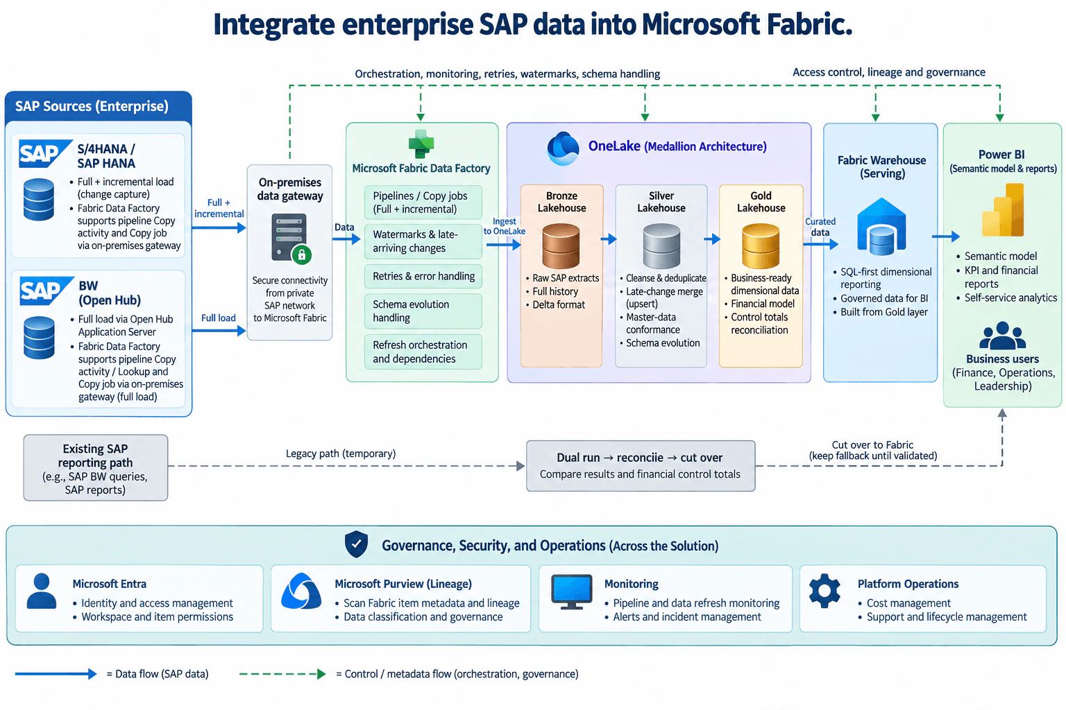
Integrate enterprise SAP data into Microsoft Fabric. diagram
How to Explain It in an Interview
1. Define the SAP extraction boundary

The production data starts in enterprise SAP systems. The diagram uses two source patterns. The S/4HANA / SAP HANA path supports an initial full load plus incremental processing. SAP BW Open Hub follows the full-load path shown in the architecture.

The on-premises data gateway sits between the private SAP network and Microsoft Fabric. It is the connectivity boundary, not a business-data store. SAP remains the source of record. Source-side authorization determines what Fabric is allowed to read.

For SAP HANA, Fabric Data Factory supports pipeline Copy activity through the on-premises gateway, and Copy job supports full and incremental loading. A pipeline can also coordinate watermark-based incremental logic when that is the chosen ingestion pattern. SAP BW Open Hub supports pipeline Copy and Lookup activity and Copy job full loading through an on-premises gateway.

If the gateway or source connection fails, only the affected source load should fail. Data Factory records the failed run. Operators correct the source, network, or gateway problem and retry from the appropriate extraction boundary instead of changing already published reports manually.

2. Use Fabric Data Factory as the shared orchestration layer

Fabric Data Factory owns pipelines, Copy jobs, dependencies, refresh sequencing, watermarks, retry behavior, error handling, and schema-handling workflow. These are shared platform capabilities, so every SAP reporting product does not rebuild them.

The orchestration layer is logically different from the production data plane. Data Factory coordinates work, while SAP business records are transported into and stored in OneLake. Scheduling metadata, run state, and control decisions should not be confused with the business records themselves.

For incremental processing, the watermark must advance only after the intended ingestion boundary succeeds. A retry should restart from a known position. Transport success alone is not enough to declare a financial dataset correct.

3. Land raw SAP data in the Bronze Lakehouse

The first durable Fabric data state is the Bronze Lakehouse in OneLake. Bronze contains raw SAP extracts, retains full history, and uses Delta-format storage as shown in the diagram.

Bronze is the replay boundary. If a Silver or Gold transformation fails, the platform can recompute the affected downstream data from Bronze instead of immediately rereading the SAP source.

Bronze is not the trusted reporting layer. Its primary responsibility is to preserve the source load and enough ingestion context to understand what arrived and when.

4. Make Silver the cleansing and conformance boundary

The Silver Lakehouse cleans and deduplicates Bronze data. It also handles late changes through merge or upsert logic, applies master-data conformance, and manages approved schema evolution.

This is where shared business entities are standardized before they are reused by reports. The exact customer, vendor, general-ledger, or other master-data rules remain domain-owned business definitions; the platform provides the reusable transformation boundary in which those rules are applied.

For a late-arriving change, Silver uses the business key and change logic to update the intended representation instead of blindly creating a duplicate. If a breaking schema change cannot be processed safely, downstream publication stops until the mapping and affected contracts are updated and validated.

5. Publish Gold only after financial validation

The Gold Lakehouse contains business-ready dimensional data and the financial model shown in the architecture. It is the curated boundary between engineering transformations and trusted serving.

Financial control totals are a publication gate. The platform compares the curated result with the agreed source-derived controls before treating Gold data as ready. The exact controls depend on the finance domain, so I would not invent their values or formulas during design.

If reconciliation fails, the technical pipeline may have completed but the business publication has not succeeded. The affected Gold result stays untrusted while the team investigates missing records, duplicate processing, master-data mappings, late changes, or transformation defects.

6. Serve Gold through Fabric Warehouse and Power BI

Curated Gold data flows into Fabric Warehouse. The Warehouse is the SQL-first dimensional reporting layer shown in the diagram and provides governed data for BI.

Power BI sits at the consumer boundary. It uses a semantic model for KPIs, financial reports, enterprise reporting, and self-service analytics for finance, operations, and leadership users.

The refresh dependency is important. SAP ingestion completes first, then Bronze-to-Silver-to-Gold processing, then financial reconciliation, then Warehouse serving, and finally the Power BI semantic-model refresh. If an upstream validation fails, the orchestration should not present that failed result as newly trusted data.

7. Apply access, lineage, monitoring, and operations across the solution

Microsoft Entra provides identity for access to Fabric. Fabric workspace and item permissions are the authorization boundary for users and workloads shown in the architecture. Network connectivity to SAP does not itself authorize access to Fabric data.

Microsoft Purview provides the governance and lineage view. A registered and scanned Fabric tenant can contribute Fabric item metadata and lineage to Purview. Purview stores governance metadata rather than the SAP production records themselves. This helps stewards and operators understand dependencies and downstream impact.

Monitoring covers pipeline state and data-refresh state, with alerts and incident handling for failures. Platform Operations owns shared lifecycle and cost management. This distinction matters operationally: a bad domain transformation is a data-product defect, while a gateway or shared orchestration outage can affect several SAP data products.

8. Handle late changes, schema evolution, retry, and replay as different problems

A retry repeats a failed orchestration step. A replay or recomputation rebuilds downstream data from Bronze. A historical backfill reads source history that is not already present in the landing layer. These are different recovery actions.

Late SAP changes flow through the incremental path and are merged in Silver using the approved business key and change rules. Schema evolution is handled at the ingestion and transformation boundary. Compatible changes can move through the approved mapping. Breaking changes stop trusted publication until downstream mappings and contracts have been validated.

Repeatedly retrying a deterministic data-quality or reconciliation defect does not help. The platform should expose the failed state, stop publication, allow the responsible team to correct the cause, then recompute from the appropriate persisted boundary.

9. Cut over with dual run, reconciliation, and fallback

The existing SAP reporting path stays active temporarily during migration. The new Fabric path runs in parallel.

The migration sequence is dual run, reconcile, then cut over. During the overlap, teams compare Fabric results with the existing SAP reports and check financial control totals. Only after the new results are validated should users move to the Fabric semantic model and reports.

The legacy path remains a fallback during the validation period. If important discrepancies appear, consumers can remain on the validated existing route while the Fabric defect is corrected. Decommissioning is a later lifecycle decision after the new reporting path has been accepted; technical deployment alone is not a sufficient cutover criterion.

10. Define ownership around reusable capabilities

The platform team owns the shared foundation represented in the diagram: gateway integration, Fabric Data Factory orchestration patterns, OneLake medallion structure, Warehouse serving patterns, Entra-based access mechanisms, Purview integration, monitoring, and platform lifecycle operations.

SAP source owners remain responsible for source authorization and source-system correctness. Domain and data owners define master-data and financial business rules. Business users consume the governed semantic models and reports.

The architecture therefore behaves as a reusable platform rather than one hard-coded pipeline. New SAP data products can reuse the same connectivity, orchestration, storage, governance, monitoring, and serving boundaries while keeping business-specific mappings and financial rules with the responsible domain.

11. Explain the main trade-offs

The first trade-off is freshness versus source and operational cost. Incremental SAP HANA loading avoids repeating every full extraction, but it requires reliable incremental state, late-change handling, and recovery logic. The BW Open Hub path shown in this design remains a full-load pattern and therefore has a different source and network cost profile.

The second trade-off is reuse versus domain autonomy. Shared Fabric patterns reduce duplicated engineering work, but data products must conform to common publication, access, lineage, and reconciliation rules before becoming trusted Gold data.

The third trade-off is migration speed versus reporting risk. Immediate replacement is simpler operationally, but dual running creates evidence that the new results agree with the established reporting path before users are moved.

The fourth trade-off is Lakehouse flexibility versus Warehouse-oriented serving. Bronze, Silver, and Gold Lakehouses provide the medallion transformation and historical-data boundaries shown in the design. Fabric Warehouse provides the SQL-first dimensional serving boundary. The architecture uses both because their responsibilities are different.

Technical Approach
  1. Inventory the SAP source paths and classify each according to the selected architecture: full plus incremental for the SAP HANA path, and full load for SAP BW Open Hub.
  2. Place the on-premises data gateway between the private SAP network and Fabric.
  3. Use Fabric Data Factory pipelines and Copy jobs as reusable ingestion and orchestration capabilities, with dependencies, incremental state, retries, error handling, schema handling, and refresh sequencing.
  4. Land source extracts in the Bronze Lakehouse and retain raw history for audit and replay.
  5. Transform Bronze to Silver by cleansing, deduplicating, merging late changes, conforming master data, and processing approved schema evolution.
  6. Build Gold dimensional and financial models and calculate the agreed financial control totals.
  7. Publish only reconciled Gold data to the Fabric Warehouse serving layer.
  8. Refresh the Power BI semantic model only after the upstream data and reconciliation gates succeed.
  9. Apply Microsoft Entra access controls, Microsoft Purview metadata and lineage governance, monitoring, and Platform Operations across the platform.
  10. Dual-run Fabric beside the existing SAP reporting path, compare results and financial controls, cut over after validation, and keep the legacy path temporarily as fallback.
Practical Insights

The first likely bottleneck is the SAP extraction and gateway boundary because the source systems, gateway, network, and concurrent loads all limit ingestion speed. Incremental SAP HANA processing can reduce repeated data movement, while the BW Open Hub path shown here uses full loads and can therefore move more repeated data. Storage grows because Bronze keeps history and Silver and Gold keep additional processed representations. Transformation work grows with table count, late-change merges, deduplication, master-data rules, schema changes, and reconciliation. Warehouse and Power BI pressure depends on the number and concurrency of reporting workloads. Operational effort grows with source contracts, failures, schema changes, and control-total rules. Migration temporarily costs more because the legacy and Fabric paths run together, but that overlap reduces cutover risk. No precise throughput, latency, storage, concurrency, or cost value should be assumed until the source and business requirements are known.

Why Interviewers Ask This

This tests whether a Data Engineer can design more than an SAP-to-Power-BI copy job. The interviewer wants to see correct source and platform boundaries, reusable ingestion, incremental-state handling, late-change processing, master-data conformance, financial reconciliation, governed serving, operational recovery, and a low-risk migration from an existing reporting estate.

Common interview mistakes

Common mistakes are treating the design as one SAP-to-Power-BI copy job; assuming every SAP connector has identical full-load and incremental capabilities; bypassing the on-premises gateway for the private SAP paths shown; advancing incremental state before the intended load boundary succeeds; treating Bronze as already-clean business data; losing raw history needed for replay; ignoring late-arriving changes; appending changed business records as duplicates instead of merging them in Silver; letting every report implement its own customer, vendor, or financial mappings; treating pipeline success as proof of financial correctness; publishing Gold when control totals fail; refreshing Power BI before upstream validation completes; allowing reports to query raw SAP extracts directly; confusing Purview governance metadata with production records; assuming authentication alone grants data access; repeatedly retrying deterministic data-quality errors; silently accepting breaking schema changes; and replacing the existing reporting path without a dual run, reconciliation gate, controlled cutover, and temporary fallback.

Interview tip

Present the design as a sequence of trust boundaries: SAP extraction, Fabric orchestration, Bronze landing, Silver conformance, Gold reconciliation, Warehouse serving, and Power BI consumption. Spend the most time on incremental state, late-change merges, master-data conformance, financial controls, refresh dependencies, and dual-run cutover because those demonstrate platform judgment rather than simple data movement.
Interviewer may ask next
What would you do if a late SAP correction changes a financial transaction after the daily Fabric load has already reached Power BI?

I would keep the same architecture and treat the correction as a source change, not as a manual report adjustment. For the incremental SAP HANA path, Data Factory reads the correction from the next valid incremental boundary and lands it in Bronze so the ingestion history remains available. Silver uses the business key and approved late-change logic to merge the corrected representation instead of creating a duplicate. Gold recomputes the affected dimensional or financial result and reruns the financial control totals. The Warehouse and Power BI semantic model should receive the corrected publication only after reconciliation passes. If a previous reporting period must be rebuilt, I would replay the affected Bronze-to-Silver-to-Gold processing rather than edit Power BI data. Monitoring exposes the delayed or failed publication to operators, while consumers continue to use the last validated reporting state.

How would you handle a breaking SAP schema change during the dual-run migration?

I would stop the affected dataset at the transformation and trusted-publication boundary instead of silently passing the new shape into Gold. The incoming extract still lands in Bronze when the source load itself is readable, preserving the changed structure for investigation and replay. The data team updates the Silver mapping and any affected master-data or financial transformation, then recomputes the downstream data and reruns reconciliation. Microsoft Purview lineage helps identify affected Fabric items and downstream dependencies within the supported lineage view. During migration, the existing reporting path remains the temporary fallback. Only after the revised Fabric result passes validation would I resume the Gold-to-Warehouse-to-Power-BI refresh sequence and continue toward cutover.

12. How does parallel copy affect Azure Data Factory transfer performance?PerformanceEasyMicrosoft

Question Details

Start with one measurable source-to-sink Copy Activity. Compare source partitioning, degree of copy parallelism, data integration units, self-hosted runtime capacity, file sizes, compression, and sink throttling; isolate the limiting stage with throughput and queue metrics rather than increasing every setting at once.

Short Interview Answer (30-60 seconds)

Parallel copy increases concurrent source reads and sink writes, so throughput can improve while enough independent work and downstream capacity are available. It stops helping when the source, Integration Runtime, network, or sink becomes the bottleneck. Measure first, then tune only the limiting stage.

Detailed Explanation

Parallel copy in Azure Data Factory increases the number of concurrent read-and-write operations used by one Copy Activity. That can improve throughput when the source exposes enough independent files or partitions, the Integration Runtime has available capacity, and the sink can accept concurrent writes. It is not an unlimited speed control: actual parallelism can be lower than the configured parallelCopies value, and throughput eventually reaches the capacity of the narrowest stage. The correct approach is to measure the same source-to-sink copy, identify that limiting stage, change one relevant lever, and retest.

Useful Questions to Ask the Interviewer
  1. Is the Copy Activity using Azure Integration Runtime or a self-hosted Integration Runtime?
  2. Is the source naturally split into multiple files or partitions that can be read independently?
  3. Is the current symptom low throughput, time spent in queue, source throttling, or sink throttling?
  4. Are we allowed to change source partitioning, file sizes, compression, Integration Runtime capacity, parallelCopies, or sink concurrency?
  5. Do we need to keep the same source data, destination, and output correctness while comparing changes?
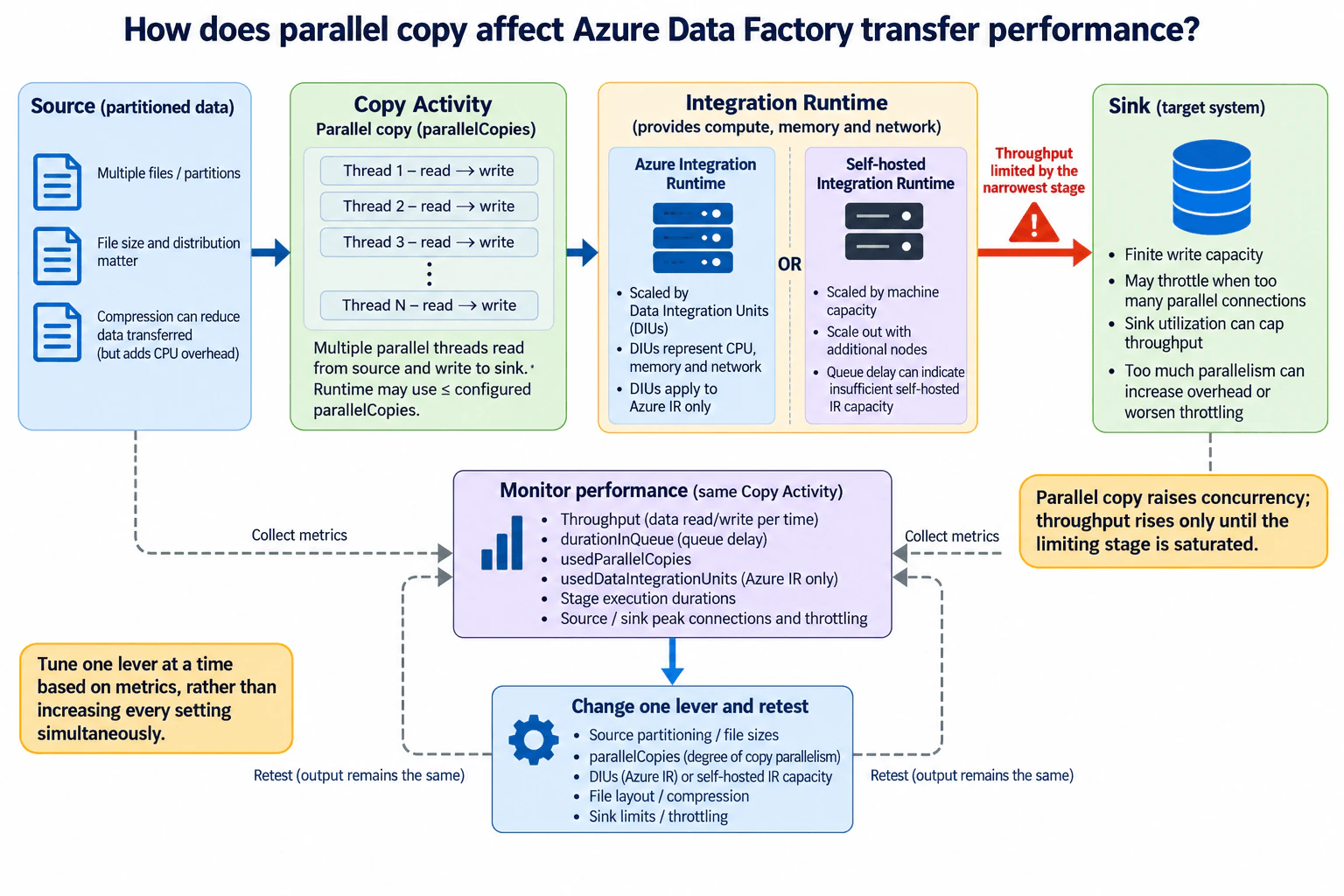
How does parallel copy affect Azure Data Factory transfer performance? diagram
How to Explain It in an Interview

Start with one measurable Copy Activity and view the transfer as a single flow from the partitioned source, through Copy Activity and the Integration Runtime, to the sink. The parallelCopies setting controls the maximum degree of copy parallelism. Multiple parallel read-and-write paths can increase throughput, but only when the source provides enough independent work and the rest of the transfer path has spare capacity. The runtime can therefore use fewer parallel copies than the configured maximum.

Source layout is the first constraint to check. Multiple files or partitions can provide independent work for concurrent reads, while poor file distribution can restrict usable parallelism. File size also affects efficiency because very small files can increase per-file overhead, while insufficiently partitioned input can leave too little work to keep parallel copy paths busy. Compression can reduce the number of bytes transferred, but compression and decompression add CPU work, so it can shift the bottleneck rather than automatically make every transfer faster.

Next, check Integration Runtime capacity. With Azure Integration Runtime, Data Integration Units represent the compute, memory, and network resources available to the copy operation. If Azure IR capacity is the limiting stage, additional useful DIU capacity can help, but increasing parallelCopies alone cannot create runtime capacity that is not available. With a self-hosted Integration Runtime, DIUs do not apply; the relevant limits are the CPU, memory, network capacity, and available nodes of the self-hosted runtime. Queue delay can indicate that the runtime does not have enough available capacity for the workload.

The sink is another independent limit. A target system has finite write capacity and can throttle when too many concurrent writes or connections arrive. Once the sink is saturated, increasing parallelCopies may only add contention, overhead, or throttling. Overall transfer throughput is therefore limited by the narrowest stage across source reads, Integration Runtime capacity, the network path, and sink writes.

Use monitoring evidence instead of increasing every setting together. For the same Copy Activity, examine throughput, durationInQueue, usedParallelCopies, usedDataIntegrationUnits when Azure Integration Runtime is used, stage execution durations, source and sink peak connections, and throttling information. These measurements help isolate whether the limiting stage is source availability, Integration Runtime capacity, network throughput, or destination write capacity.

Then change one principal lever that matches the evidence: source partitioning or file sizes, parallelCopies, Azure Integration Runtime DIUs, self-hosted Integration Runtime capacity, file layout or compression, or sink limits and throttling. Run the same workload again, compare the same measurements, and verify that the output remains equivalent. The key trade-off is that additional concurrency improves throughput only until another stage becomes saturated; beyond that point it can increase resource use and downstream pressure without reducing transfer time.

Technical Approach
  1. Run one representative source-to-sink Copy Activity and confirm that its output is correct.
  2. Record the target metric, primarily transfer throughput and total copy duration.
  3. Inspect throughput, durationInQueue, usedParallelCopies, stage execution durations, source and sink peak connections, and throttling evidence; also inspect usedDataIntegrationUnits when Azure Integration Runtime is used.
  4. Identify the narrowest stage: source read parallelism, Integration Runtime capacity, network path, or sink write capacity.
  5. If the source is limiting, examine source partitioning, file count, file-size distribution, and compression behavior.
  6. If Azure Integration Runtime capacity is limiting, evaluate DIU capacity. If self-hosted Integration Runtime is limiting, evaluate machine or node CPU, memory, network capacity, and queue delay.
  7. If useful copy concurrency is limiting and the surrounding stages still have spare capacity, adjust parallelCopies.
  8. If the sink is limiting, address its write capacity, connection limits, or throttling instead of adding more copy parallelism.
  9. Change only one principal lever, rerun the same workload, and compare the same metrics.
  10. Validate equivalent output and stop increasing parallelism once another stage becomes the bottleneck.
Practical Insights

There is no meaningful Big-O complexity calculation for this configuration question. The important costs are physical resource and external-system capacity. More parallel copy paths can consume more source connections, Integration Runtime CPU, memory, and network bandwidth, and more sink connections or write capacity. Azure Integration Runtime capacity is represented by DIUs, while self-hosted Integration Runtime performance depends on its own machine and node resources. Compression can reduce transferred bytes but increase CPU work. Small-file overhead can waste time, while too little independent source work can prevent configured parallelism from being used. Once the source, runtime, network, or sink is saturated, additional concurrency mainly adds overhead or throttling rather than throughput.

Why Interviewers Ask This

Interviewers want to see whether you understand that Azure Data Factory Copy Activity performance is an end-to-end capacity problem, not simply a matter of choosing a large parallelCopies value. A strong answer connects source partitioning, actual copy parallelism, Azure Integration Runtime DIUs or self-hosted Integration Runtime capacity, file sizes, compression, sink throttling, and measured throughput or queue evidence before choosing a tuning change.

Common interview mistakes

Common mistakes are setting parallelCopies very high without proving that the source has enough independent work; assuming configured parallelism equals actual parallelism; treating DIUs as a self-hosted Integration Runtime setting; increasing DIUs, parallelCopies, file count, runtime capacity, and sink concurrency at the same time so the useful change cannot be identified; ignoring file-size distribution and compression CPU cost; overlooking sink connection limits or throttling; using only total duration instead of queue and stage-level evidence; and assuming that more parallelism must make the copy faster after another stage is already saturated.

Interview tip

Frame the answer around the bottleneck: parallel copy raises concurrency, but throughput improves only while the source, Integration Runtime, network, and sink have spare capacity. Mention the ADF monitoring metrics, distinguish Azure IR DIUs from self-hosted IR capacity, and finish by saying you change one lever and retest the same workload.

Interviewer may ask next
What would you check if increasing parallelCopies does not improve Copy Activity throughput?

First check usedParallelCopies to see whether the requested concurrency is actually being used. Then inspect source partitioning and file distribution, stage execution durations, durationInQueue, Integration Runtime capacity, network behavior, source and sink peak connections, and throttling. If the source has too little independent work, the runtime is capacity-constrained, the network is saturated, or the sink is already at its write limit, a higher parallelCopies setting will not improve throughput. Tune the measured limiting stage and rerun the same workload.

How does tuning differ between Azure Integration Runtime and self-hosted Integration Runtime?

With Azure Integration Runtime, DIUs represent the compute, memory, and network resources available to the copy operation, so usedDataIntegrationUnits is relevant when diagnosing capacity. DIUs do not apply to a self-hosted Integration Runtime. For self-hosted IR, examine the CPU, memory, network capacity, and available nodes of the runtime and look for queue delay that can indicate insufficient available capacity. In both cases, verify source parallelism and sink limits before adding runtime resources.

13. Select one preferred customer contact from three prioritized fields.CodingEasyMicrosoft

Question Details

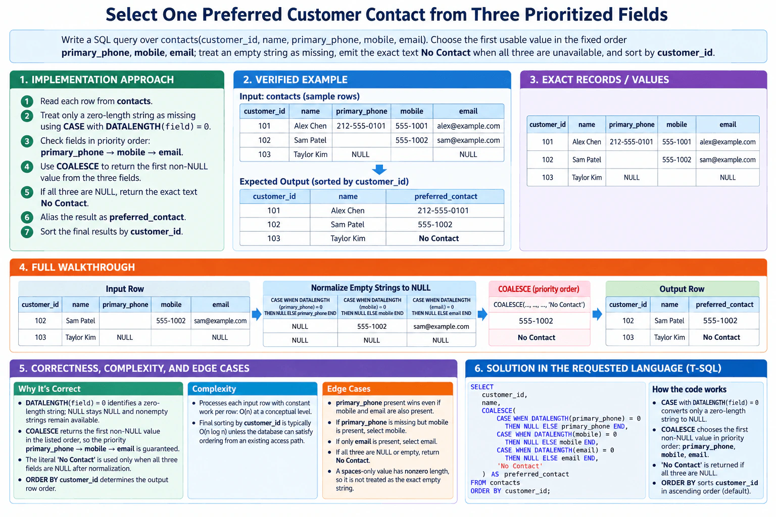
Write a SQL query over contacts(customer_id, name, primary_phone, mobile, email). Choose the first usable value in the fixed order primary_phone, mobile, email; treat an empty string as missing, emit the exact text No Contact when all three are unavailable, and sort by customer_id. Example: a customer with blank primary_phone, mobile 555-1002, and an email must return 555-1002; a customer with all three blank or NULL must return No Contact.

Short Interview Answer (30-60 seconds)

I would normalize only true zero-length strings to NULL, then use COALESCE in the required priority order: primary_phone, mobile, then email. I use DATALENGTH(field) = 0 inside CASE so a spaces-only value is not treated as an empty string. If every contact field is unavailable, COALESCE returns 'No Contact'. Finally, I sort by customer_id. The per-row selection work is O(n), and the required sort is typically O(n log n). The contact expression uses O(1) extra space per row.

Detailed Explanation

See the Code while reading this explanation.

The contacts table has one row per customer and three possible contact values. We must choose one preferred value. The priority is fixed: primary_phone first, then mobile, then email. A true empty string counts as missing. A value containing spaces is not the same as a zero-length string in this implementation. If all three contact values are unavailable, the output must contain the exact text No Contact. The final rows must be sorted by customer_id.

Useful Questions to Ask the Interviewer
  1. Should only a zero-length string count as empty, or should whitespace-only values also count as missing?
  2. Should the result include customer_id and name together with preferred_contact, as shown in the expected output?
Select one preferred customer contact from three prioritized fields. diagram
How to Explain It in an Interview
1. Understand the input and required output

The input is contacts(customer_id, name, primary_phone, mobile, email). The result keeps customer_id and name and adds preferred_contact. For each customer, preferred_contact must be the first usable value in this exact order: primary_phone, mobile, email. If none is usable, it must be No Contact. The result is sorted by customer_id.

2. Normalize exact empty strings

For each contact field, I use CASE with DATALENGTH(field) = 0. A true zero-length string becomes NULL. A NULL input remains NULL because the ELSE branch returns the original NULL value. A nonempty value remains unchanged. A spaces-only string has nonzero length, so it is not treated as the exact empty string.

3. Select the first usable contact

I pass the normalized primary_phone, mobile, and email expressions to COALESCE in that exact order. COALESCE returns the first value that is not NULL. This makes primary_phone the first choice, mobile the second choice, and email the third choice. The final COALESCE argument is the exact literal 'No Contact'.

4. Walk through the verified example

Customer 101, Alex Chen, has primary_phone 212-555-0101, mobile 555-1001, and alex@example.com. The primary phone is usable, so preferred_contact is 212-555-0101.

Customer 102, Sam Patel, has a blank primary_phone, mobile 555-1002, and sam@example.com. The blank primary_phone becomes NULL. Mobile is then the first non-NULL value, so preferred_contact is 555-1002.

Customer 103, Taylor Kim, has no usable primary_phone, mobile, or email. After normalization, all three are NULL. COALESCE therefore returns No Contact.

5. Explain why the result is correct

The key invariant is that each value given to COALESCE is either the original usable contact value or NULL when that field is unavailable. The COALESCE argument order is identical to the required business priority. Therefore its first non-NULL result is exactly the preferred contact. The final 'No Contact' literal handles the case where all three contact fields are unavailable.

6. Explain the T-SQL implementation

The SELECT returns customer_id and name. Each contact column is wrapped in CASE WHEN DATALENGTH(column) = 0 THEN NULL ELSE column END. Those normalized values go into COALESCE in the order primary_phone, mobile, email. The result is aliased as preferred_contact. The query reads from contacts and finishes with ORDER BY customer_id.

7. Explain complexity and edge cases

For n rows, the contact-selection expressions perform a constant amount of work per row, so that part is O(n). The required ORDER BY customer_id is typically O(n log n) when an explicit sort is needed. If the database can already produce rows in customer_id order through an appropriate access path, that sorting work may be avoided. The contact expression uses O(1) extra space per row. Important cases are a present primary phone, missing primary with present mobile, email as the only usable field, all three fields unavailable, and a spaces-only value.

Key Insight / Why This Solution Works

The solution has two stages. First, normalize each contact field so a true zero-length string becomes NULL while other nonempty values stay unchanged. The central invariant is that every expression passed to COALESCE is either the original usable value or NULL when that field is unavailable. Second, use COALESCE in the exact priority order primary_phone, mobile, email, followed by 'No Contact'. Because the argument order matches the required priority, the first non-NULL result is the correct preferred contact.

Code
-- Return each customer with one preferred contact value.
SELECT
  customer_id,
  name,
  COALESCE(
    -- Treat only a true zero-length primary phone as missing.
    CASE
      WHEN DATALENGTH (primary_phone) = 0 THEN NULL
      ELSE primary_phone
    END,
    -- If primary_phone is unavailable, try mobile next.
    CASE
      WHEN DATALENGTH (mobile) = 0 THEN NULL
      ELSE mobile
    END,
    -- If both phone fields are unavailable, try email.
    CASE
      WHEN DATALENGTH (email) = 0 THEN NULL
      ELSE email
    END,
    -- Use the required exact fallback when all contact fields are unavailable.
    'No Contact'
  ) AS preferred_contact
FROM
  contacts
  -- Return the final rows in customer_id order.
ORDER BY
  customer_id;
Time & Space Complexity

Let n be the number of contact rows. The CASE and COALESCE expressions do a fixed amount of work for each row, so the contact-selection part is O(n). The query must also sort by customer_id. A general sort is typically O(n log n), so the complete query is typically O(n log n) when a sort is required. If the database can already return rows in customer_id order from a suitable access path, the explicit sorting work may be avoided. The contact expression uses O(1) extra space per row, while a database sort may use working memory that grows with the result size.

Where it is used

This SQL pattern is useful when data has several fallback fields with a fixed business priority. Common examples include choosing a preferred phone number, selecting the first available customer identifier, choosing a backup address, or selecting the first usable value from several nullable source-system columns.

Why Interviewers Ask This

This question checks whether a candidate can translate a business priority rule into correct SQL. It tests understanding of NULL versus an empty string, ordered fallback logic with COALESCE, exact output requirements, and result ordering with ORDER BY. It also shows whether the candidate can keep the SQL readable, explain why the priority is correct, handle the all-missing case, and discuss the cost of the required sort accurately.

Common interview mistakes

A common mistake is checking the fields in the wrong order, such as mobile before primary_phone. Another is passing empty strings directly to COALESCE, because an empty string is still non-NULL and could be selected incorrectly. For the implementation shown in the diagram, candidates should also avoid changing the rule so that spaces-only values are silently treated as empty. Other mistakes are returning different fallback text instead of the exact No Contact value, forgetting ORDER BY customer_id, or describing only the O(n) per-row work while ignoring the possible O(n log n) sort.

Interview tip

Explain the query as two simple stages: first convert only true empty strings to NULL, then let COALESCE apply the priority primary_phone → mobile → email → 'No Contact'. This makes both the code and the correctness argument easy to follow.

Interviewer may ask next
How would the query change if whitespace-only values should also count as missing?

I would change only the normalization step. Before COALESCE, each field would be converted to NULL when it contains no meaningful characters according to the agreed whitespace rule. The priority order would remain primary_phone, mobile, email, then 'No Contact'. Correctness is preserved because every value considered unusable becomes NULL before COALESCE chooses the first remaining value. The per-row processing remains O(n) across n rows, and ORDER BY is still typically O(n log n) when sorting is required. The tradeoff is more normalization work and the need to define exactly which whitespace characters count as empty.

What changes if the output does not need to be sorted by customer_id?

The preferred-contact logic does not change. I would remove only ORDER BY customer_id and keep the same CASE expressions and COALESCE priority. Each row would still produce the same preferred_contact value. Without the required final sort, the contact-selection work is O(n) across n rows and uses O(1) extra space per row. The tradeoff is that the database no longer guarantees the order in which the result rows are returned.

14. Calculate dataset freshness status against per-dataset service-level limits.CodingMediumMicrosoft

Question Details

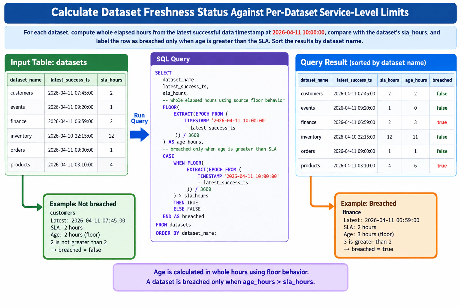
Write a SQL query that evaluates each dataset at the fixed current timestamp 2026-04-11 10:00:00. Compute whole elapsed hours from the latest successful data timestamp using the source-defined floor behavior, compare that age with sla_hours, label the row breached only when age is greater than the SLA, and sort by dataset name. Example: a latest timestamp of 2026-04-11 07:45 with sla_hours=2 has age_hours=2 and is not breached, while a timestamp of 06:59 has age_hours=3 and is breached.

Short Interview Answer (30-60 seconds)

I would calculate each dataset’s age from the fixed timestamp 2026-04-11 10:00:00. In PostgreSQL, I subtract latest_success_ts, extract the elapsed seconds, divide by 3600, and apply FLOOR so partial hours round down. Then I compare age_hours with sla_hours. A row is breached only when age_hours is strictly greater than the SLA. Finally, I sort by dataset_name. The row calculations are O(n), and the required sort can make the overall work O(n log n).

Detailed Explanation

See the Code while reading this explanation.

The table contains one row for each dataset. Each row has the dataset name, the latest successful data time, and the allowed age in hours. We compare every row with the same fixed time, 2026-04-11 10:00:00. We convert the elapsed time into whole hours by rounding down. Then we mark a dataset as breached only when that whole-hour age is greater than its SLA. The query keeps one output row for each input row and sorts the final result by dataset name.

Useful Questions to Ask the Interviewer
  1. Should I use PostgreSQL timestamp and interval behavior, as shown in the supplied solution?
  2. Should a dataset that exactly reaches its SLA remain not breached? The stated rule says yes.
  3. Can latest_success_ts ever be later than the fixed evaluation timestamp?
Calculate dataset freshness status against per-dataset service-level limits. diagram
How to Explain It in an Interview
1. Understand the input and output

The input table is datasets. Each row contains dataset_name, latest_success_ts, and sla_hours. The output keeps those three fields and adds age_hours and breached. The result remains one row per dataset. The rows must be sorted by dataset_name.

2. Calculate whole elapsed hours

For each row, subtract latest_success_ts from TIMESTAMP '2026-04-11 10:00:00'. PostgreSQL returns an interval. EXTRACT(EPOCH FROM ...) converts the interval into elapsed seconds. Divide by 3600 to convert seconds to hours. FLOOR removes the fractional part so the query uses whole elapsed hours with the required floor behavior.

For customers, 10:00 minus 07:45 is 2 hours 15 minutes, or 8,100 seconds. 8,100 / 3,600 = 2.25, so FLOOR gives age_hours = 2.

For finance, 10:00 minus 06:59 is 3 hours 1 minute, or 10,860 seconds. 10,860 / 3,600 is about 3.0167, so FLOOR gives age_hours = 3.

3. Apply the SLA rule

The CASE expression uses a strict greater-than comparison. A row is breached only when the floored age is greater than sla_hours. Equality is not a breach.

For customers, age_hours is 2 and sla_hours is 2. The condition 2 > 2 is false, so breached is false.

For finance, age_hours is 3 and sla_hours is 2. The condition 3 > 2 is true, so breached is true.

4. Walk through the complete example

The supplied diagram contains six rows. customers at 07:45 with SLA 2 produces age_hours 2 and breached false. events at 09:20 with SLA 1 produces age_hours 0 and breached false. finance at 06:59 with SLA 2 produces age_hours 3 and breached true. inventory at 22:15 on the previous day with SLA 12 produces age_hours 11 and breached false. orders at 09:00 with SLA 1 produces age_hours 1 and breached false. products at 03:10 with SLA 4 produces age_hours 6 and breached true.

5. Explain why the result is correct

Every row uses the same fixed evaluation timestamp. The query first measures the true elapsed interval, converts it to hours, and applies FLOOR. The breach decision then uses that same floored expression and the strict rule age_hours > sla_hours. This is why customers is not breached at age 2 with SLA 2, while finance is breached at age 3 with SLA 2.

6. Explain the PostgreSQL query

The SELECT reads each dataset row and computes age_hours directly. The same floor expression is used again inside CASE so the breached value follows the exact same age calculation. TRUE is returned only when the calculated age is greater than sla_hours. FALSE is returned otherwise. FROM datasets preserves the input grain, and ORDER BY dataset_name produces the required sorted output.

Key Insight / Why This Solution Works

The key idea is to calculate one floored whole-hour age for each dataset at the same fixed timestamp, then apply a strict SLA comparison. The elapsed interval is converted to seconds with EXTRACT(EPOCH FROM ...), divided by 3600, and passed to FLOOR. The central invariant is that the displayed age and the breach decision use the same floor-based elapsed-hour rule. A dataset is breached only when that whole-hour age is greater than sla_hours, never when it is equal.

Code
SELECT
  dataset_name,
  latest_success_ts,
  sla_hours,
  -- Convert the elapsed interval to seconds, then floor to whole hours.
  FLOOR(
    EXTRACT(
      EPOCH
      FROM
        (
          TIMESTAMP '2026-04-11 10:00:00' - latest_success_ts
        )
    ) / 3600
  ) AS age_hours,
  -- A dataset is breached only when the same floored age exceeds its SLA.
  CASE
    WHEN FLOOR(
      EXTRACT(
        EPOCH
        FROM
          (
            TIMESTAMP '2026-04-11 10:00:00' - latest_success_ts
          )
      ) / 3600
    ) > sla_hours THEN TRUE
    ELSE FALSE
  END AS breached
FROM
  datasets
  -- Return the required alphabetical ordering.
ORDER BY
  dataset_name;
Time & Space Complexity

Let n be the number of dataset rows. The timestamp calculation and SLA comparison do constant work for each row, so evaluating the rows is O(n). The required ORDER BY dataset_name may require sorting, which is typically O(n log n) when the database must perform a separate sort. Extra working memory depends on the database execution plan and the sort implementation.

Where it is used

This SQL pattern is useful for data freshness monitoring. A data platform can store the latest successful load timestamp and an SLA for each dataset, then run a query like this to identify stale data. The result can feed an operations dashboard, scheduled health report, or alerting process while keeping different freshness limits for different datasets.

Why Interviewers Ask This

This question tests whether you can translate an operational freshness rule into precise SQL. The interviewer is checking timestamp arithmetic, floor behavior, boundary conditions, CASE logic, result grain, and sorting. It also tests whether you notice that equality with the SLA is allowed and whether you consistently use one fixed evaluation timestamp for every dataset instead of accidentally changing the time during the calculation.

Common interview mistakes

A common mistake is using normal rounding instead of FLOOR, which changes partial-hour behavior. Another mistake is comparing the exact fractional age with sla_hours instead of comparing the floored whole-hour value. Using >= instead of > is also wrong because a dataset exactly at its SLA is not breached. Candidates may also use a changing current timestamp instead of the required fixed timestamp. Finally, forgetting ORDER BY dataset_name would produce the wrong required ordering.

Interview tip

Use the customers row to explain the boundary clearly: 07:45 to 10:00 is 2.25 hours, FLOOR makes the age 2, and 2 > 2 is false. Then contrast it with finance, where 06:59 to 10:00 floors to 3 hours and 3 > 2 is true.

Interviewer may ask next
How would the query change if the evaluation time should use the real current database time instead of the fixed timestamp?

Replace the fixed TIMESTAMP '2026-04-11 10:00:00' expression with the required PostgreSQL current-time expression, while keeping the same subtraction, EXTRACT(EPOCH), division by 3600, FLOOR, and strict greater-than comparison. The correctness rule stays the same: compute the whole-hour age first, then mark the row breached only when that age is greater than sla_hours. Row evaluation remains O(n), with the same possible O(n log n) sorting cost.

What should happen if latest_success_ts is later than the evaluation timestamp?

With the shown formula, the elapsed interval becomes negative, so FLOOR produces a negative age_hours value. That value would normally not be greater than a positive SLA, so breached would be false. If future timestamps represent invalid data, I would add a separate validation rule or status rather than silently changing the freshness formula. That keeps the original freshness calculation correct while making bad timestamps visible.

15. Join labels to the feature values that were available at label time.CodingHardMicrosoft

Question Details

Write a point-in-time SQL join between label rows and versioned feature rows. For each label, select the most recent feature timestamp on or before that label timestamp for the same entity; do not use a later feature, preserve labels with no eligible feature by returning NULL feature values, and resolve source-defined ties deterministically. Example: features 12 at 09:00 and 15 at 11:00 joined to a 10:00 label return 12, while an 08:00 label returns NULL.

Short Interview Answer (30-60 seconds)

I would keep every label row and use a correlated OUTER APPLY to find its point-in-time feature. For each label, I filter to the same entity and require feature_ts <= label_ts, so no future feature can leak in. TOP (1) orders by feature_ts DESC and then the source-defined feature_version_id tie-breaker. If no feature qualifies, OUTER APPLY returns NULL feature columns. There is no plan-independent Big-O bound; runtime and workspace depend on SQL Server indexes and the execution plan.

Detailed Explanation

See the Code while reading this explanation.

Each label represents a moment when we need the feature information that was already available at that time. We must never use a feature that appeared later because that would bring future information into an earlier label. For each label, we therefore consider only feature rows for the same entity whose timestamp is at or before the label timestamp. We choose the newest eligible row. If no eligible feature exists, we still keep the label and return NULL feature values.

Useful Questions to Ask the Interviewer
  1. Which source-defined column should break ties when two feature rows have the same feature timestamp?
  2. Should every input label row produce exactly one output row?
  3. Is an index on the feature lookup columns available or allowed?
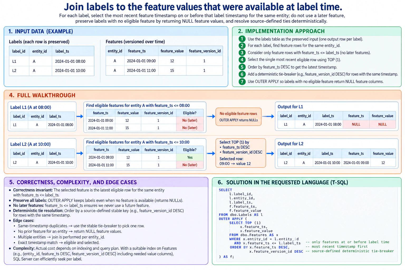
Join labels to the feature values that were available at label time. diagram
How to Explain It in an Interview
1. Understand the input and required output

The labels table contains label_id, entity_id, and label_ts. Every label row must remain in the result. The features table contains entity_id, feature_ts, feature_value, and feature_version_id. For each label, we need at most one feature row. The feature must belong to the same entity and must have feature_ts <= label_ts. If no feature satisfies those rules, the feature columns must be NULL.

2. Choose the point-in-time join

I use T-SQL OUTER APPLY with a correlated TOP (1) query. For the current label, the inner query looks only at rows with the same entity_id and feature_ts <= label_ts. It orders those rows by feature_ts DESC so the newest eligible feature comes first. For rows with the same feature timestamp, feature_version_id DESC is the source-defined deterministic tie-breaker shown in the diagram.

3. Preserve labels with no eligible feature

OUTER APPLY preserves the label row even when its inner query returns no feature. In that case, the columns from the APPLY result are NULL. This is why a label before the first available feature is not dropped.

4. Walk through the exact example

Entity A has feature value 12 at 09:00 and feature value 15 at 11:00. Label L1 is at 08:00. Both feature rows are later than 08:00, so neither is eligible. The result for L1 therefore has NULL feature_ts and NULL feature_value. Label L2 is at 10:00. The 09:00 feature is eligible because 09:00 <= 10:00. The 11:00 feature is too late. TOP (1) selects the 09:00 row, so L2 receives feature value 12.

5. Explain why the result is correct

The invariant is that any selected feature is the newest eligible feature for the same entity at the label time. The WHERE clause removes future features. ORDER BY feature_ts DESC puts the newest eligible timestamp first. The source-defined feature_version_id tie-breaker makes equal feature timestamps deterministic. TOP (1) returns one feature row, and OUTER APPLY keeps the label when no row qualifies.

6. Explain the T-SQL implementation

The outer query reads dbo.Labels as l. OUTER APPLY runs a feature lookup for each label. The predicates x.entity_id = l.entity_id and x.feature_ts <= l.label_ts enforce entity matching and point-in-time eligibility. ORDER BY x.feature_ts DESC, x.feature_version_id DESC ranks the preferred eligible row first. TOP (1) returns that row. The final SELECT returns the label columns with the selected feature timestamp and value.

7. Explain performance and edge cases

This SQL statement does not have one fixed plan-independent Big-O runtime or auxiliary-space bound because SQL Server can choose different execution plans. Performance depends on data size, indexes, statistics, and the chosen operators. A suitable feature index beginning with entity_id and feature_ts, with the deterministic tie-breaker available and feature_value covered when useful, can make each correlated lookup much more efficient. Important cases are no prior feature, multiple entities, an exact timestamp match, and duplicate feature timestamps that need the source-defined tie-breaker.

Key Insight / Why This Solution Works

The key idea is an as-of, or point-in-time, lookup for each label. The label row is preserved. For that label, consider only feature rows for the same entity where feature_ts <= label_ts. Sort those eligible rows by feature_ts descending so the newest available timestamp is first. If several rows share that timestamp, use the source-defined feature_version_id descending tie-breaker shown in the diagram. TOP (1) selects one row. OUTER APPLY keeps the label and produces NULL feature columns when no row is eligible. The invariant is that any selected feature is the latest eligible feature for that entity at label time.

Code
-- Preserve every label row in the output.
SELECT
  l.label_id,
  l.entity_id,
  l.label_ts,
  f.feature_ts,
  f.feature_value
FROM
  dbo.Labels AS l OUTER APPLY (
    -- For this label, return only the preferred eligible feature row.
    SELECT
      TOP (1) x.feature_ts,
      x.feature_value
    FROM
      dbo.Features AS x
    WHERE
      -- Match features only from the same entity.
      x.entity_id = l.entity_id
      -- Prevent future-data leakage by using only features available by label time.
      AND x.feature_ts <= l.label_ts
    ORDER BY
      -- Choose the most recent eligible feature timestamp first.
      x.feature_ts DESC,
      -- Resolve equal timestamps with the source-defined deterministic tie-breaker.
      x.feature_version_id DESC
  ) AS f;
Time & Space Complexity

There is no single plan-independent Big-O time or auxiliary-space bound for this T-SQL query. SQL Server chooses an execution plan using the table sizes, indexes, statistics, and available resources. Without a useful feature index, repeated correlated searches may require much more work. With an index that supports entity_id, feature_ts, and the deterministic tie-breaker, SQL Server can efficiently locate the newest eligible row for each label. Extra memory is also execution-plan dependent because operators such as sorts, spools, scans, or seeks may use different amounts of workspace.

Where it is used

This point-in-time join pattern is useful in machine-learning feature generation, historical reporting, pricing history, account-state reconstruction, event enrichment, and other temporal data pipelines. It is used whenever a row must be matched with the newest version of data that was actually available at that historical moment. The main benefit is preventing future information from leaking into past results.

Why Interviewers Ask This

This question tests whether you understand point-in-time correctness in data pipelines. The interviewer wants to see whether you can prevent future-data leakage, preserve the required label grain, handle missing historical features, and resolve equal timestamps deterministically. It also tests practical T-SQL knowledge, including correlated OUTER APPLY, TOP with ORDER BY, and the effect of indexing and execution plans on performance.

Common interview mistakes

One mistake is matching the nearest timestamp without enforcing feature_ts <= label_ts, which can use a future feature. Another is using CROSS APPLY or an inner join and accidentally dropping labels that have no eligible feature. A third is finding one maximum feature timestamp for an entity without correlating it to each label timestamp. Candidates may also forget the source-defined tie-breaker when several feature rows have the same timestamp. Finally, ordering feature_ts ascending would select the oldest eligible feature instead of the newest one.

Interview tip

Start by saying, "I will never allow feature_ts to be later than label_ts." Then explain that OUTER APPLY preserves unmatched labels and that TOP (1) with descending timestamp returns the latest feature that was actually available.

Interviewer may ask next
How would you handle two feature rows for the same entity with exactly the same feature_ts?

I would keep feature_ts DESC as the first ordering key and then use the source-defined deterministic tie-breaker. In the shown solution, that is feature_version_id DESC. TOP (1) then selects the preferred row among equal timestamps. The point-in-time correctness rule does not change because both rows are still required to satisfy feature_ts <= label_ts. Performance and workspace remain execution-plan dependent.

How would you improve performance when the features table is very large?

I would keep the same OUTER APPLY logic and add an index that supports the correlated lookup. The index should begin with entity_id and feature_ts, with the source-defined tie-breaker available in the ordering and feature_value covered when useful. This helps SQL Server narrow the search to the correct entity and find the newest eligible row efficiently. Correctness does not change because the predicates and ordering remain the same. The tradeoff is additional index storage and extra maintenance work on feature writes.

Disclaimer: This interview guide is for educational and informational purposes only. It is designed to help readers prepare, but it does not guarantee any interview result, hiring decision, offer, or outcome. Interview questions, hiring criteria, and preferred answers can vary by employer, interviewer, industry, location, and time. The examples and explanations reflect the authors' research and judgment, are provided without warranties of any kind, and should not be treated as the only correct approach. Diagrams are simplified illustrations intended to highlight the main components and their interactions; actual systems and implementations may be more complex. Alternative approaches may be equally valid or better suited to a particular question, context, or interviewer. To the fullest extent permitted by applicable law, the author, contributors, and publisher are not liable for decisions made, actions taken, or losses incurred based on this guide.

Company Notice: This guide is an independent educational resource and is not affiliated with, endorsed by, sponsored by, or approved by the company named in this guide. Company names are used only to identify interview experiences commonly reported by candidates. Interview practices can change without notice, and inclusion of company-specific content does not mean these questions are official, complete, or guaranteed to be asked. To the fullest extent permitted by law, the author, contributors, and publisher are not responsible for outcomes related to use of this material.

Content Accuracy and Verification: To the fullest extent permitted by applicable law, we do not represent or warrant that interview guides, questions, answers, examples, or diagrams are accurate, complete, current, error-free, or suitable for any particular purpose. You are responsible for independently reviewing and verifying the information before relying on it.