NVIDIA DevOps Engineer Interview Questions & Answers

I would trace one representative read end to end, timestamp every boundary, and compare it with a healthy cohort. I would inspect client queues, node pressure, network, storage services, retries, and GPU transfer, then validate the first boundary that becomes abnormal before changing configuration.

The goal is to find where a slow dataset read first starts losing time. I would follow the same piece of data from the training program until it is ready for use, recording the time at each step. I would compare that journey with a similar run that is working normally. This shows whether the delay begins on the training machine, while the data is traveling, or while storage is finding and returning it. I would gather proof first, test the suspected area, make only the smallest justified change, and repeat the same test afterward.

1. Is the 200 ms value an end-to-end read-latency target, and which percentile matters most: p50, p95, or p99?
2. Can I compare the affected workload with healthy runs using the same dataset, job type, model, cluster, path, and similar load?
3. What storage interface is involved, such as a filesystem, object store, or block storage?
4. Are synchronized clocks and per-boundary timestamps already available across the application, nodes, network, and storage services?
5. Is GPU starvation visible as part of the impact, or is the reported symptom limited to dataset-read latency?

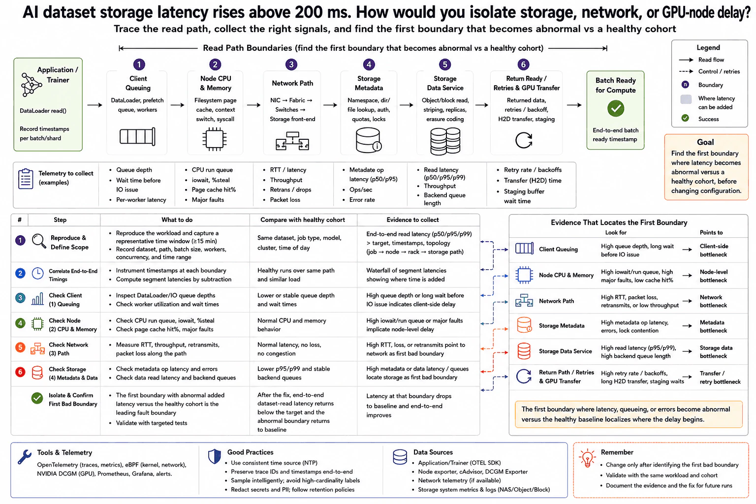
I would start with the user-visible objective: dataset reads are persistently above the 200 ms target, so I need to locate the first boundary where the read path becomes abnormal. I would not immediately tune storage, networking, or the GPU node.

First, I would reproduce a representative slow read during a controlled time window. I would preserve the dataset, path, batch size, worker count, concurrency, topology, and timestamps. I would use a consistent clock source across systems so clock skew does not create a false latency boundary.

At the application and client boundary, I would measure DataLoader or prefetch queue depth, worker wait time, and per-worker latency. A large queue or long wait before I/O begins points toward a client-side bottleneck rather than remote storage.

At the GPU node, I would check CPU run queue, I/O wait, steal time, page-cache behavior, and major page faults. High run queue, I/O wait, or major faults compared with a healthy node can explain delay before the network path is reached.

For the network path, I would inspect round-trip time, throughput, retransmissions or drops, and packet loss across the NIC, fabric, switches, and storage front end. High RTT, loss, retransmissions, or unexpectedly low throughput relative to healthy runs makes the network the leading fault boundary.

For storage, I would separate metadata work from data reads. Metadata evidence includes lookup latency, operations per second, error rate, and lock contention. Data-service evidence includes p50, p95, and p99 read latency, throughput, backend queue length, and errors. This separation matters because slow namespace or metadata work can look like slow storage even when the data service itself is healthy.

On the return path, I would check retry rate and backoffs, then measure host-to-device transfer time and staging-buffer wait. High retries can amplify delay, while long H2D transfer or staging waits can localize the problem to the GPU-host transfer path instead of storage.

I would correlate all of these signals with consistent timestamps and bounded resource attributes such as job, node, rack, storage path, and workload cohort. Application instrumentation creates request or read timing. OpenTelemetry traces and metrics can carry correlation context; a collector can receive, enrich, sample when appropriate, and transport telemetry to the configured backend. Prometheus-style metrics provide aggregate trends, while traces or timestamped events provide per-read timing. eBPF and operating-system signals add kernel and network evidence, and NVIDIA DCGM provides GPU-related health and utilization signals. Dashboards query the stored telemetry so operators can compare the current path with healthy cohorts. No one signal alone proves root cause.

The main SLI is end-to-end dataset-read latency, normally viewed with percentiles such as p50, p95, and p99. Supporting SLIs include queue wait, network RTT and loss, metadata-operation latency, data-service latency, retry rate, throughput, and H2D transfer time. The SLO should define acceptable end-to-end behavior before alert thresholds are chosen. Alerts should be symptom based and actionable, with an owner, severity, runbook context, and a sustained condition or other noise control.

The key diagnostic step is to build a timestamped latency waterfall and compare each boundary with the healthy baseline. The first boundary where latency, queueing, errors, throughput, or utilization becomes abnormal localizes where the delay begins. I would treat that as the leading fault boundary, then collect targeted evidence to confirm the hypothesis and reject alternatives that remain healthy.

Telemetry has limits. High-cardinality labels increase ingestion and storage cost, so I would keep dimensions bounded. Detailed traces may be sampled to control overhead, but sampling can miss rare slow reads; targeted or tail-aware sampling can be useful during diagnosis when supported. Retention should be long enough for incident comparison without wasting storage. Missing telemetry or clock skew must be treated as uncertainty, not evidence. Credentials, tokens, personal data, and sensitive payloads must be redacted.

Because the question does not provide a confirmed root cause, I would not invent a specific configuration change. After evidence confirms the fault boundary, I would apply the smallest safe correction appropriate to that evidence. Then I would rerun the same workload and trace. Success means the previously abnormal boundary returns toward the healthy baseline and end-to-end dataset-read latency returns below the defined target without new errors or throughput regressions.

Finally, I would keep dashboards for boundary latency, queues, errors, retries, throughput, and GPU transfer, and test alerts with controlled conditions so operators know the dashboard and alerting path reflects real service health. This preserves the same evidence trail for future incidents.

1. Define end-to-end dataset-read latency as the main SLI and agree on the target or SLO before choosing alert thresholds.
2. Reproduce one representative slow read while preserving dataset, path, batch size, worker count, concurrency, topology, and time range.
3. Use synchronized timestamps and common resource attributes so application, node, network, storage, and GPU-transfer evidence can be correlated.
4. Measure client queue depth, worker wait time, and per-worker read latency.
5. Measure GPU-node CPU run queue, I/O wait, steal time, page-cache behavior, and major page faults.
6. Measure network RTT, throughput, retransmissions or drops, and packet loss along the NIC-to-storage path.
7. Separate storage metadata from data services. Measure metadata latency, operations per second, errors, and lock contention separately from data-read latency, throughput, and backend queues.
8. Measure retry rate, backoffs, host-to-device transfer time, and staging-buffer waits on the return path.
9. Build a timestamped latency waterfall and compare each boundary with a healthy cohort using the same path and similar load.
10. Identify the first boundary where latency, queueing, errors, throughput, or utilization becomes abnormal. Treat it as the leading fault boundary, not automatically as proven root cause.
11. Collect targeted evidence to validate that hypothesis and reject alternatives that remain healthy.
12. Apply only the smallest evidence-supported correction.
13. Rerun the same read and verify that the abnormal boundary returns toward baseline and end-to-end latency returns below the target.
14. Keep dashboards and actionable alerts for the important boundary signals to detect recurrence.

The investigation adds measurement cost because timestamps, metrics, traces, operating-system signals, and GPU signals must be collected, transported, stored, and queried. High-cardinality labels can make telemetry expensive, so labels should stay bounded. Detailed tracing and eBPF collection can add overhead, so sampling and limited diagnostic windows may be needed. Sampling can miss rare slow reads, while long retention increases storage cost. Maintaining synchronized clocks, dashboards, alerts, and healthy baselines also requires ongoing operational work, but it makes future diagnosis faster and reduces unsafe configuration changes.

Common mistakes are blaming storage only because the symptom is called storage latency; changing configuration before collecting evidence; using only averages instead of useful percentiles; failing to separate client queueing, GPU-node delay, network delay, metadata latency, data-service latency, retries, and H2D transfer; comparing unrelated workloads instead of a healthy cohort; using unsynchronized clocks; assuming one metric proves root cause; creating high-cardinality telemetry; ignoring sampling bias, missing telemetry, or retention limits; and declaring success without rerunning the same workload and verifying both the boundary and end-to-end latency.

Present the diagnosis as a boundary-by-boundary evidence flow. Say that you will preserve timestamps and topology, compare against a healthy cohort, find the first abnormal boundary, validate it with another signal, and only then make the smallest safe change. This shows disciplined troubleshooting instead of guessing.

I would suspect a masked partial Service data-plane failure. Existing connections may survive while kube-proxy cycles, but new connections, failover, scaling, or endpoint changes can expose broken rules, conntrack pressure, or unhealthy eBPF replacement state. I would correlate evidence first and prove recovery with fresh cross-node connection tests.

The danger is that everything can look normal because old connections are still working. A part of the system that sends users to healthy application instances may be unstable on some machines. Nothing may fail until a new request needs a fresh path, traffic moves to another machine, an application instance changes, or the system grows. I would find why the repeated restarts happen, compare affected and healthy machines, check whether traffic instructions are correct, and actively create fresh connections from several places. I would call the system recovered only after the restarts stop and those tests remain successful.

1. Is the cluster using kube-proxy with iptables or IPVS, or has an eBPF implementation replaced kube-proxy Service handling?
2. Are the restarts limited to particular nodes, zones, node images, or Kubernetes versions?
3. Were there recent kube-proxy, CNI, kernel, node-image, ConfigMap, NetworkPolicy, Service, EndpointSlice, or resource-limit changes?
4. Have fresh connections been tested across affected nodes, or do we only know that existing traffic is still succeeding?

The hidden risk is an intermittent or partial Kubernetes Service data-plane failure. Application Pods can be healthy while node-level Service forwarding is unstable. Existing TCP connections can continue through already-programmed forwarding state and conntrack, so they may hide a problem that affects fresh flows. The failure can suddenly appear during a new connection, endpoint update, rollout, scale event, node drain, failover, or traffic shift.

I would not conclude that kube-proxy restarts are harmless simply because current traffic succeeds. Repeated restarts on several nodes are a data-plane warning until fresh Service programming and new connections are proven healthy.

First I would identify which kube-proxy Pods and nodes are cycling, when the behavior started, and whether restart counts are still increasing. I would collect Pod status, the previous termination state, Kubernetes events, and previous-container logs before making changes.

Useful commands include kubectl get pods -n kube-system -l k8s-app=kube-proxy -o wide, kubectl describe pod, kubectl get events, and kubectl logs --previous. I would look for OOM kills, probe failures, configuration errors, permission failures, fatal runtime errors, or other restart reasons. A restart reason is evidence, not automatically the complete root cause.

Because several nodes are affected, I would correlate kube-proxy restarts with node conditions and capacity. I would inspect memory and CPU pressure, DiskPressure, PIDPressure, Ready state, eviction activity, kernel messages, and kube-proxy resource requests and limits.

For example, repeated OOMKilled terminations together with memory pressure or an undersized container limit would strongly support a resource hypothesis. I would also compare affected and healthy nodes to see whether the issue follows a node pool, image, kernel version, zone, or capacity class.

I would inspect the kube-proxy ConfigMap and DaemonSet arguments, proxy mode, kube-proxy image, Kubernetes version, CNI configuration, and recent deployment history. I would compare affected nodes with known-good nodes rather than assuming every node received the same effective configuration.

With standard kube-proxy, I would determine whether Service forwarding uses iptables or IPVS. If an eBPF implementation has replaced kube-proxy Service handling, I would inspect that implementation's agent health, attached programs, service maps, and backend maps instead of treating kube-proxy as the active forwarding component.

For iptables or IPVS mode, I would verify that expected Service rules or virtual-server state exists on affected nodes and that programmed destinations match the current ready backends. Missing, stale, or partially programmed state can leave some traffic paths working while others fail.

For an eBPF replacement, I would verify that the expected programs are attached and that Service and backend maps are loaded and synchronized. The important question is not simply whether kube-proxy is running. The question is whether the component actually responsible for Service forwarding has programmed correct state.

I would inspect EndpointSlices and compare their ready endpoint addresses and topology information with the backends actually programmed on affected nodes. I would also look for endpoint churn around the restart period.

A Service can exist and application Pods can look healthy while a node still has stale or incomplete forwarding state. Low endpoint churn can hide that stale state for a while; a later rollout, scale event, or failover may force reprogramming and expose the defect.

Conntrack is important because it helps explain why existing traffic may survive. Once a connection is established, packets can continue using existing connection-tracking and forwarding state even while new Service programming is unhealthy.

I would inspect conntrack utilization, configured limits, insertion failures or drops where observable, and cleanup behavior. A nearly exhausted or unhealthy conntrack table can make new connections fail while long-lived sessions continue.

Then I would deliberately compare established connections with fresh connections. I would create new TCP connections from multiple clients and nodes. If long-lived connections succeed while fresh connections time out or fail intermittently, that strongly supports a masked data-plane, topology, or conntrack problem.

I would test from multiple nodes and, where relevant, multiple zones so that one fortunate path does not hide a partial outage. I would compare node-local and cross-node paths and account for topology-aware routing when it is enabled.

I would correlate the incident timeline with cluster upgrades, kube-proxy changes, CNI or eBPF-agent changes, node-image or kernel updates, ConfigMap changes, NetworkPolicy changes, Service or EndpointSlice changes, firewall or sysctl changes, and resource-request or limit changes. A recent change is only a hypothesis until the evidence supports it.

The correction must follow the confirmed cause. If kube-proxy is OOM-killed, I would correct inappropriate resource limits or node capacity. If conntrack is exhausted, I would address capacity, workload behavior, or timeout configuration rather than blindly changing a limit. If configuration or version mismatch caused the restarts, I would restore a compatible known-good configuration or version.

If iptables or IPVS programming is failing, I would correct the underlying programming dependency or configuration. If an eBPF replacement is unhealthy, I would repair its agent, maps, programs, or use its documented safe fallback. If EndpointSlices or backend state are wrong, I would correct the underlying endpoint or synchronization issue. If a recent change is strongly correlated and increases risk, rollback or containment may be safer than continuing deep diagnosis in place.

Healthy application Pods are not sufficient evidence of recovery. I would require kube-proxy Pods to remain Running and stable on nodes where kube-proxy is the active Service implementation, with restart counts no longer increasing and no recurring OOM, probe, or configuration failures. If an eBPF replacement owns Service forwarding, its agents and programmed state must remain healthy instead.

I would verify that iptables or IPVS state, or eBPF Service and backend maps, matches the expected endpoints. EndpointSlices must show the expected ready backends. Conntrack must have safe headroom without continuing exhaustion symptoms.

Most importantly, I would run synthetic probes that create new connections through the Service from representative nodes and zones. I would check success, latency, errors, and backend reachability. This avoids the false confidence created by long-lived established connections.

The smallest useful signal set is kube-proxy restart and termination state, Kubernetes events, previous kube-proxy logs, node conditions and resource metrics, active Service-programming state, EndpointSlice readiness, conntrack health, and fresh-connection synthetic probe results. I would correlate them by cluster, node, zone, Service, workload, and time where those attributes are available.

A useful user-facing SLI is fresh Service connection success: successful synthetic new connections divided by attempted synthetic new connections across representative paths. A supporting operational SLI is the proportion of expected nodes whose active Service-programming state matches current ready backends. I would define the SLO from the Service reliability requirement before choosing alert thresholds.

Alerts should be symptom-based and actionable. Examples are repeated kube-proxy restarts across nodes, OOM kills, sustained conntrack saturation, missing or stale Service-programming state, and failed fresh-connection probes. Each alert should include ownership, severity, affected scope, and runbook context. Appropriate durations or aggregation should prevent normal rollout or endpoint churn from creating unnecessary noise.

A dashboard should correlate restart rate, termination reasons, node pressure, conntrack utilization, programmed rule or map health, EndpointSlice readiness, synthetic fresh-connection success, Service error rate, and latency. Prometheus-style metrics provide health and trend signals. Kubernetes events and structured logs provide reasons and context. eBPF tools expose data-plane state when eBPF is actually in use. Grafana or an equivalent dashboard layer can correlate these signals. Traces can help when application request paths are instrumented, but they do not replace node-level Service-state checks or synthetic probes.

Metrics should avoid unbounded high-cardinality labels such as individual connection IDs. Logs should have deliberate retention and must redact credentials, tokens, personal data, and sensitive payloads. Missing telemetry must be detectable because an absent metric, silent exporter, or failed collector must not be interpreted as healthy service behavior.

The interview takeaway is simple: correlate across layers. Observe the restart, preserve evidence, narrow the boundary, test competing hypotheses, apply the smallest safe correction, and prove recovery using fresh traffic rather than relying on workloads that merely look healthy.

1. Scope the cycling kube-proxy Pods by node, zone, restart count, and start time.
2. Preserve restart evidence: termination state, Kubernetes events, previous logs, and restart reasons.
3. Correlate node conditions, resource pressure, OOM events, kernel signals, and kube-proxy limits.
4. Compare kube-proxy configuration, proxy mode, image, Kubernetes version, CNI configuration, and recent changes with healthy nodes.
5. Inspect the active Service data plane: iptables/IPVS state when kube-proxy owns forwarding, or eBPF programs and Service/backend maps when kube-proxy replacement is enabled.
6. Compare EndpointSlices and ready backend addresses with the destinations programmed on affected nodes.
7. Inspect conntrack utilization and failure indicators, then compare established sessions with intentionally created new connections.
8. Test Service access from multiple nodes and zones to expose topology-dependent or partial failures.
9. Use correlated evidence to identify the cause and apply the smallest safe correction or rollback.
10. Verify stable forwarding components, correct rules or maps, healthy EndpointSlices, conntrack headroom, and successful fresh synthetic connections during an observation window.

This is an operational investigation rather than an algorithm with meaningful Big-O complexity. The main cost is collecting and comparing evidence across nodes, Service state, EndpointSlices, conntrack, logs, events, and synthetic paths. In a large cluster, start with affected nodes and representative Services, then widen the scope if evidence suggests a broader problem. Metrics are relatively cheap but need bounded label cardinality. Detailed logs and data-plane diagnostics cost storage and operator time. Synthetic probes add a small amount of traffic, but they provide direct evidence that new connections work. Dashboards, alerting, capacity planning, version baselines, and tested runbooks reduce ongoing maintenance effort.

Common mistakes are assuming healthy application Pods prove the Service data plane is healthy; looking only at the current kube-proxy log instead of the previous crashed container; treating restart count alone as the root cause; ignoring node OOM or pressure; inspecting kube-proxy's iptables/IPVS state when an eBPF implementation actually replaced kube-proxy Service handling; checking EndpointSlices without comparing them with programmed backends; ignoring conntrack because established sessions still work; testing only long-lived connections; testing from only one node or zone; blaming the most recent change without evidence; changing several settings at once; blindly raising conntrack limits; and declaring recovery as soon as Pods become Running without proving fresh connections.

Lead with the hidden risk: established traffic can mask an unstable or partially broken Service data plane. Then walk through restart evidence, node health, configuration, the active iptables/IPVS or eBPF forwarding state, EndpointSlices, conntrack, fresh versus established connections, topology, and recent changes. Finish with the smallest evidence-based correction and proactive cross-node fresh-connection tests that prove recovery before users experience the failure.