156 Data Analyst Interview Questions & Answers

88 top • 10 Accenture • 10 Bank of America • 10 Capital One • 9 Deloitte • 9 JPMorgan Chase • 10 Target • 10 Walmart

Data Analyst icon

Questions with Detailed ExplanationsWith Detailed Explanations

(Last Updated: September 13, 2026)

41. Compare Type I and Type II errors in a business decision.Statistics And ExperimentationMedium

Question Details

Discuss the different consequences of Type I and Type II errors and the tension between significance thresholds and power.

Short Interview Answer (30-60 seconds)

A Type I error is a false positive: we reject a true null hypothesis and may launch a change that does not really improve the business metric. Its probability is controlled by the significance level, alpha. A Type II error is a false negative: we fail to reject a false null hypothesis and miss a real improvement. Its probability is beta, and power is 1 minus beta. With sample size and effect size fixed, lowering alpha reduces Type I errors but generally increases Type II errors and lowers power. I would choose alpha and sample size based on the relative business cost of both errors and also consider practical significance.

Detailed Explanation

Type I and Type II errors describe two ways a statistical business decision can be wrong. A Type I error is a false positive: we conclude that a change works when there is actually no real effect. A Type II error is a false negative: we miss a real improvement. The significance level, alpha, controls the Type I error rate, while beta represents the Type II error rate and statistical power equals 1 minus beta. The right balance depends on the business cost of unnecessary action versus the cost of missing a valuable opportunity.

Useful Questions to Ask the Interviewer
  1. Which mistake is more costly for this decision: launching an ineffective change or missing a real improvement?
  2. What outcome metric defines success, and what size of improvement would be practically meaningful?
  3. What population and unit are being randomized or observed?
  4. What significance threshold and target power should be planned before looking at the results?
  5. Is there enough sample size and experiment duration to detect the business-relevant effect?
  6. Are there risks such as selection bias, confounding, attrition, interference, repeated peeking, or multiple testing?
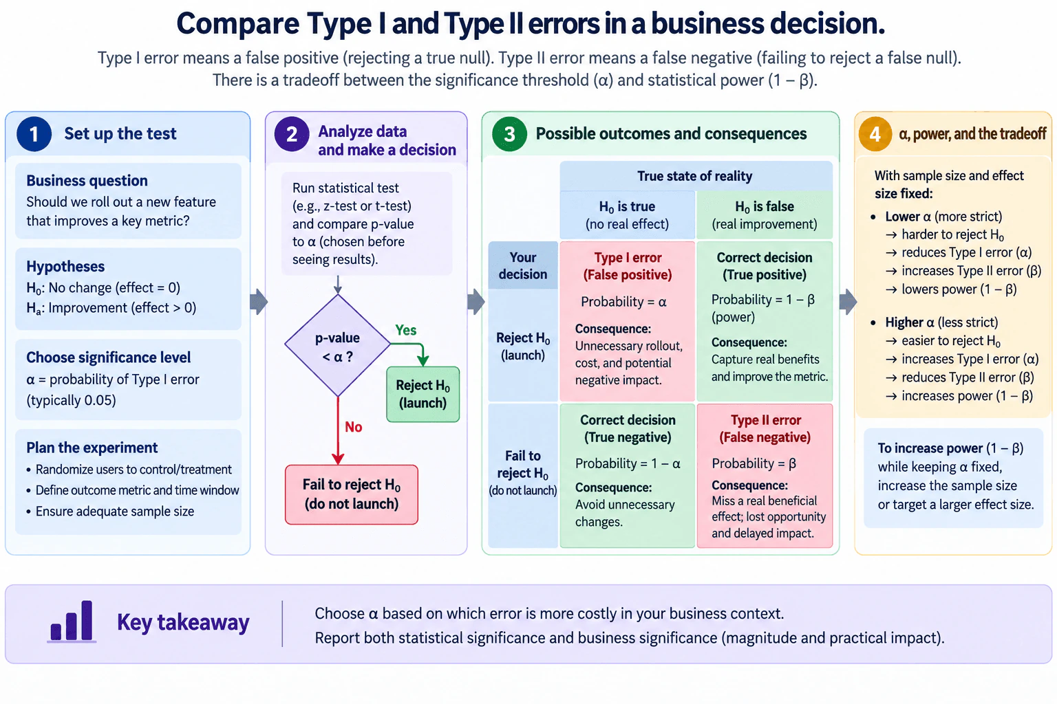
Compare Type I and Type II errors in a business decision. diagram
How to Explain It in an Interview

Start with the hypotheses. In the business example shown in the diagram, the null hypothesis, H0, represents no real improvement in the key outcome metric, while the alternative hypothesis, Ha, represents an improvement. Before testing, I would define the outcome metric, population, randomization unit, time window, practically meaningful effect, and significance level.

A Type I error happens when H0 is actually true but I reject it. This is the false-positive case. In the diagram's example, that could mean launching a feature that has no real improvement, creating unnecessary rollout cost, wasted effort, or possible negative impact. The significance level alpha sets the allowed probability of this error under the null hypothesis for the specified test.

A Type II error happens when H0 is false but I fail to reject it. This is the false-negative case. The business may decide not to launch even though a real improvement exists, so it may lose potential benefits, revenue, or customer value. The probability of this error is beta for a specified true alternative. Statistical power is 1 minus beta, which is the probability of rejecting H0 when that specified alternative is true.

The diagram shows the four possible outcomes. If H0 is true and we reject it, that is a Type I error with probability alpha. If H0 is true and we fail to reject it, that is the corresponding correct decision, with probability 1 minus alpha when the test has exact size alpha. If H0 is false and we reject it, that is a correct detection, with probability equal to the test's power for that alternative. If H0 is false and we fail to reject it, that is a Type II error with probability beta.

The significance threshold creates an important tradeoff. If sample size, effect size, variability, and the test procedure are held fixed, lowering alpha makes the test more strict. It becomes harder to reject H0, so Type I error risk decreases, but beta generally increases and power decreases. Raising alpha makes rejection easier, increasing Type I error risk while generally reducing beta and increasing power.

This does not mean the only way to get more power is to accept a larger alpha. If I want higher power while keeping alpha fixed, I can often increase the sample size. Power can also improve when the true effect is larger or the measurement is less noisy. That is why sample-size and power planning should happen before reading the experiment result.

After the experiment, I would compare the p value with the preselected alpha as part of the hypothesis-test decision. A p value smaller than alpha leads to rejecting H0 under that decision rule, while a larger p value means failing to reject H0. I would not interpret the p value as the effect size or as the probability that H0 is true.

I would also report the estimated effect and a confidence interval so stakeholders can see the magnitude and uncertainty. Statistical significance tells us whether the observed evidence crosses the chosen testing threshold. Practical significance asks whether the size of the effect is large enough to matter to the business. A statistically significant result can still be too small to justify a rollout.

Before recommending a launch, I would verify that randomization worked as intended, sample size and exposure were adequate, the analysis used the correct unit, and there was no important attrition, interference, selection bias, confounding, repeated peeking, or uncorrected multiple testing. These problems can invalidate the intended error-rate guarantees or make the conclusion unreliable.

The final business decision should therefore combine statistical evidence with the relative cost of the two mistakes. If a false positive would be especially costly, I may choose a stricter alpha and compensate with a larger sample when feasible. If missing a real improvement is especially costly, I may prioritize greater power. In either case, I would communicate the effect estimate, uncertainty, statistical significance, practical significance, and the consequences of both Type I and Type II errors.

Technical Approach
  1. Define the business decision, outcome metric, population, randomization or observation unit, time window, and practically meaningful effect.
  2. State H0 and Ha clearly.
  3. Choose alpha before examining the results based partly on the cost of a false positive.
  4. Plan sample size for adequate power against a business-relevant effect while keeping alpha fixed.
  5. Check randomization, sample size, data quality, attrition, interference, bias, confounding, peeking, and multiple testing.
  6. Run the appropriate statistical test and compare the p value with the preselected alpha.
  7. Interpret all four possible decision states, including Type I error alpha and Type II error beta.
  8. Report the effect estimate and confidence interval, separating statistical significance from practical significance.
  9. Make the business decision using both statistical evidence and the relative costs of false positives and false negatives.
Practical Insights

The main cost is not computational complexity but decision risk and experiment resources. A lower alpha reduces false-positive risk but, with other factors fixed, generally lowers power and increases false-negative risk. Increasing sample size can raise power while keeping alpha fixed, but it requires more users, observations, time, or experiment cost. A larger true effect is easier to detect than a smaller one. The best design balances these statistical tradeoffs with the business cost of each possible mistake.

Why Interviewers Ask This

Interviewers want to see whether you understand the two main error types in hypothesis testing, can translate them into business consequences, and can reason about the tradeoff between the significance threshold, statistical power, sample size, and practical business value.

Common interview mistakes

Common mistakes are saying a Type I error means accepting a false null instead of rejecting a true null; saying a Type II error proves the null is true; forgetting that power equals 1 minus beta; assuming alpha and beta can both be reduced just by changing the threshold while sample size and effect size stay fixed; interpreting a p value as an effect size or as the probability that the null hypothesis is true; ignoring sample-size planning; and treating statistical significance as sufficient evidence of business value. Another mistake is trusting nominal error rates when randomization, independence assumptions, attrition, interference, repeated peeking, or multiple testing have been mishandled.

Interview tip

Use one simple business example and walk through the four outcomes. Then state the key tradeoff: with sample size and effect size fixed, a stricter alpha reduces false positives but generally lowers power. Finish by explaining that a larger sample can increase power without relaxing alpha and that the business decision should consider both statistical and practical significance.
Interviewer may ask next
What would you check before trusting the stated Type I error rate and statistical power in an A/B test?

I would check that the experiment design and analysis match the assumptions behind those rates. That includes correct randomization, the correct unit of analysis, enough planned sample size and duration, reliable outcome measurement, limited attrition and interference, and an analysis plan chosen before examining the results. I would also check for repeated peeking and multiple comparisons because mishandling them can inflate the effective Type I error rate. Finally, I would confirm that the power calculation was based on a realistic business-relevant effect and appropriate variability assumptions.

Suppose the business says both false positives and false negatives are very costly. How would you reduce both without simply changing alpha?

I would increase the amount or quality of information in the experiment. The most direct option is often a larger sample size, which can increase power while keeping alpha fixed. I would also improve measurement quality and reduce avoidable variance where the design allows, because less noise makes real effects easier to distinguish. I would define the smallest business-relevant effect before the test and size the experiment around it. I would not promise that both error probabilities can be made arbitrarily small without cost; reducing both generally requires more data, better measurement, a stronger design, or an effect that is easier to detect.

42. When does CUPED improve experimental precision, and when might it offer little benefit?Statistics And ExperimentationHard

Question Details

Discuss the role and usefulness of pre-experiment observations.

Short Interview Answer (30-60 seconds)

CUPED improves precision when a pre-experiment metric is available for many of the same randomized units, is measured before treatment, and strongly predicts the experiment outcome. It adjusts the outcome using Y_adj = Y - theta(X - X_bar), where theta is typically Cov(X,Y) / Var(X). In the simple one-covariate case, the remaining variance is reduced by a factor related to 1 - rho^2, so stronger pre/post correlation means smaller standard errors, narrower confidence intervals, and higher statistical power. CUPED offers little benefit when correlation is weak, coverage is poor, the pre-period is unrepresentative, or behavior is unstable.

Detailed Explanation

CUPED, or Controlled-experiment Using Pre-Experiment Data, uses observations collected before treatment to remove predictable user-to-user variation from an experiment outcome. The goal is not to change the true treatment effect, but to estimate it more precisely. It works best when many of the same randomized units have a reliable pre-period measure X that strongly predicts the in-experiment outcome Y. If that relationship is weak, many units lack historical observations, the historical window does not represent the experiment period, or behavior changes substantially over time, CUPED may provide little precision benefit.

Useful Questions to Ask the Interviewer
  1. Is the pre-experiment metric available for most of the same units that are randomized into treatment and control?
  2. Was X measured entirely before treatment exposure, so treatment cannot affect it?
  3. How strongly does the pre-period metric predict the experiment outcome Y?
  4. Is that pre/post relationship stable, or could seasonality or product changes make the historical window unrepresentative?
  5. How should units with missing pre-experiment observations be handled, and could that change the analysis population?
  6. What treatment-effect estimand and confidence level should be reported after adjustment?
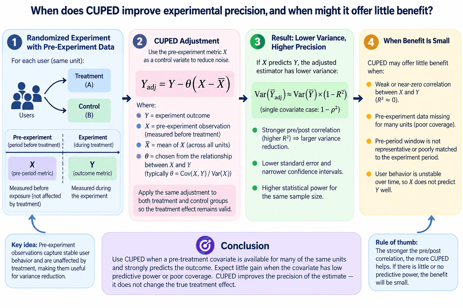
When does CUPED improve experimental precision, and when might it offer little benefit? diagram
How to Explain It in an Interview

Start with the randomized experiment. The same type of unit, such as a user, is assigned to treatment or control. For each unit, X is measured in a pre-experiment period and Y is measured during the experiment. Because X is observed before exposure, it should be unaffected by treatment.

CUPED treats X as a control variate and forms an adjusted outcome:

Y_adj = Y - theta(X - X_bar)

Here, X_bar is the mean of X across the experiment units. In the standard single-covariate linear adjustment, theta is typically chosen as:

theta = Cov(X,Y) / Var(X)

The same adjustment rule is applied to treatment and control. The treatment effect is then estimated by comparing the adjusted outcomes between the randomized groups.

The intuition is that X captures stable differences between units. Some users naturally have higher activity or spend than others regardless of treatment. If their pre-experiment behavior predicts their experiment-period behavior, CUPED subtracts part of that predictable variation. This reduces noise while leaving the treatment comparison intact under the valid randomized design and pre-treatment-covariate assumptions.

The amount of precision gain depends mainly on predictive strength. In the simple one-covariate optimal linear case, the adjusted variance is related to the original variance by a factor of approximately 1 - rho^2, where rho is the correlation between X and Y. Equivalently, this may be written using the regression R-squared for that single predictor. A stronger pre/post relationship therefore produces a larger variance reduction.

Lower variance means a lower standard error. At the same confidence level, that produces a narrower confidence interval around the estimated treatment effect. It also increases statistical power for a fixed sample size, making a real effect easier to detect without claiming that the effect itself became larger.

CUPED offers little benefit when X has weak or near-zero correlation with Y. If rho is close to zero, 1 - rho^2 is close to one, so very little variance is removed. Historical data existing by itself is not enough; it must predict the experiment outcome.

Poor pre-period coverage is another limitation. If many randomized units have no historical observations, such as new users, CUPED may have less useful information available. Simply dropping those units could also change the population being analyzed, so missingness needs an explicit, consistent treatment.

The historical window also needs to be relevant. A pre-period that is poorly matched to the experiment period can have low predictive value because of seasonality, product changes, market shifts, or other behavior changes. Similarly, when individual behavior is unstable over time, X will not predict Y well and CUPED will provide little gain.

Before interpreting the adjusted result, I would verify randomization, treatment and control sample sizes, pre-period coverage, missing-data handling, and that X was measured before treatment. I would compare the unadjusted and CUPED-adjusted treatment-effect estimates and inspect the change in estimated variance, standard error, and confidence-interval width.

If hypothesis testing is part of the experiment, the null and alternative hypotheses do not change because of CUPED. For example, the null can remain that the treatment effect is zero and the alternative that it is nonzero. CUPED changes the precision of the estimator used to evaluate those hypotheses. A smaller standard error or p value does not imply a larger business effect, so statistical significance still needs to be separated from practical significance.

The conclusion is: use CUPED when a reliable pre-treatment covariate is available for many of the same randomized units and strongly predicts the outcome. Expect little benefit when predictive power is weak, historical coverage is poor, the pre-period is not representative, or user behavior is unstable. CUPED is a variance-reduction technique: it improves the precision of the treatment-effect estimate rather than changing the underlying treatment effect.

Technical Approach
  1. Define the randomized unit, treatment and control groups, outcome Y, experiment window, and treatment-effect estimand.
  2. Identify a pre-treatment covariate X measured for the same units before exposure.
  3. Verify that treatment cannot affect X and inspect pre-period coverage and missingness.
  4. Check how strongly X predicts Y and whether that relationship is stable and representative of the experiment period.
  5. Estimate theta, typically Cov(X,Y) / Var(X) for one linear covariate.
  6. Compute X_bar across the experiment units and calculate Y_adj = Y - theta(X - X_bar) using the same adjustment rule for treatment and control.
  7. Estimate the treatment effect from the adjusted outcomes and calculate its standard error and confidence interval.
  8. Compare adjusted versus unadjusted variance or standard error to measure the precision gain.
  9. Validate randomization, sample size, missing-data handling, and sensitivity to the chosen pre-period window.
  10. Report the treatment effect and its uncertainty separately from the amount of variance reduction.
Practical Insights

The basic one-covariate CUPED calculation is inexpensive. Each unit needs a pre-period value and an experiment-period outcome, followed by mean, covariance, variance, and adjusted-outcome calculations. The harder work is usually data preparation and validation. A longer historical window may improve prediction for some metrics but can reduce coverage for newer units or become less representative. CUPED also adds analytical complexity, so if the pre/post relationship is very weak, the small precision gain may not justify the extra work.

Why Interviewers Ask This

This tests whether the candidate understands why pre-experiment observations can reduce variance in a randomized experiment, what makes a covariate useful, and when CUPED adds little value. A strong answer should connect predictive correlation to variance reduction while recognizing requirements such as pre-treatment measurement, adequate coverage, a representative historical window, valid randomization, and unchanged causal interpretation.

Common interview mistakes

Common mistakes include assuming any historical metric will help; using a covariate with weak predictive correlation; using information that can be affected by treatment; applying different adjustment logic to treatment and control; dropping units with missing pre-period data without considering selection effects; choosing a historical window that is not representative because of seasonality or behavior changes; claiming CUPED increases the treatment effect rather than its precision; interpreting a smaller p value as a larger effect; and reporting variance reduction without checking randomization, sample sizes, coverage, standard errors, and confidence intervals.

Interview tip

Explain CUPED in three steps: measure a pre-treatment X that predicts Y, subtract the predictable component from Y using the same rule in both randomized groups, and compare treatment with control using the lower-variance adjusted outcome. Then state the boundary clearly: strong pre/post predictiveness gives meaningful precision gain; weak correlation, poor coverage, or an unrepresentative pre-period gives little benefit.

Interviewer may ask next
What assumption would concern you most if the pre-experiment covariate is very strongly correlated with the outcome?

I would first verify that the covariate is genuinely pre-treatment and cannot be influenced by treatment assignment or exposure. Strong correlation is valuable for precision, but it does not make a contaminated post-treatment variable safe. I would also check that the relationship is real rather than caused by a data-processing issue, that it is reasonably stable across randomized groups, and that missingness or eligibility rules have not changed the analysis population.

What would you do if half of the randomized users have no pre-experiment observations?

I would not automatically exclude them, because that could change the target population and create selection concerns. I would measure coverage separately for treatment and control, investigate why the observations are missing, and define a consistent missing-data strategy before examining treatment lift. I would also compare CUPED with the unadjusted analysis. With poor historical coverage, the practical precision gain may be small, especially if uncovered units differ systematically from covered units or if X is only weakly predictive of Y.

43. How would you limit false discoveries across 20 concurrent experiments without overlooking real effects?Statistics And ExperimentationHard

Short Interview Answer (30-60 seconds)

I would pre-specify the primary hypotheses, decide which of the 20 tests belong to the same multiple-testing family, and verify randomization and statistical power before reading the results. When some false discoveries are tolerable and the goal is to retain sensitivity to real effects, I would usually control the false discovery rate with Benjamini-Hochberg rather than use a more conservative family-wise correction such as Bonferroni. I would also report effect sizes and confidence intervals, account for dependence among concurrent experiments, prevent unplanned peeking or selective reporting, and separate statistical significance from practical significance.

Detailed Explanation

Running 20 experiments at the same time creates a multiple-testing problem: every additional hypothesis gives another opportunity for a chance result to look statistically significant. I would first define which primary hypotheses belong to the same decision family, then use a correction that limits false discoveries while preserving enough statistical power to detect real effects. When an occasional false discovery is tolerable, false discovery rate control is usually a better balance than a very strict family-wise correction. I would combine that correction with pre-specified outcomes, sound randomization, power planning, effect sizes, confidence intervals, and transparent reporting.

Useful Questions to Ask the Interviewer
  1. Are the 20 experiments part of one coordinated decision process, or do they answer separate questions?
  2. Does each experiment have one pre-specified primary outcome, or are several metrics tested within each experiment?
  3. Is the priority to avoid even one false positive, or to control the proportion of false discoveries among selected results?
  4. Can the same unit, such as a user, participate in multiple experiments at the same time?
  5. Were sample sizes and minimum detectable effects planned before the experiments started?
  6. Are results evaluated only at a fixed endpoint, or is sequential monitoring allowed?
How to Explain It in an Interview

I would start by defining the testing family. A multiple-testing family is the set of hypotheses for which I want a joint error guarantee. I would define that family before looking at outcomes. If the 20 primary experiment hypotheses support the same decision process, treating them as one family is reasonable. If they represent genuinely separate inferential decisions, the family definition may differ, but that choice should be justified in advance rather than selected after seeing which results are favorable.

For each experiment, I would state the null and alternative hypotheses clearly. The null hypothesis says that the treatment has no effect on the pre-specified primary outcome relative to the comparison condition. The alternative says that an effect exists in the direction or form specified by the design. The estimated effect measures the size of the observed difference. The p value measures how incompatible the observed data are with the null hypothesis under the statistical model and assumptions; it is not the effect size and is not the probability that the null hypothesis is true.

If I tested all 20 hypotheses independently at an ordinary per-test significance threshold without correction, I would create more opportunities for chance findings. One solution is family-wise error rate control. Bonferroni, for example, uses a stricter per-test threshold so that the probability of making one or more false rejections across the family is bounded at the chosen family-wise level under its usual assumptions. The advantage is strong protection against false positives. The disadvantage is reduced statistical power, so genuine effects can be harder to detect.

Because the question specifically asks how to limit false discoveries without overlooking real effects, I would usually prefer false discovery rate control when the consequences of an occasional false discovery are acceptable. The false discovery rate is the expected proportion of false rejections among all rejected hypotheses, with the proportion conventionally treated as zero when there are no rejections. This criterion is less strict than family-wise error control and generally retains more power.

A standard choice is the Benjamini-Hochberg procedure. Let m=20 and choose the target false discovery rate q before examining the results. I would sort the 20 valid primary-test p values from smallest to largest: p(1) through p(20). For each rank i, compare p(i) with (i/20)q. I then find the largest rank k for which p(k) is less than or equal to (k/20)q. If such a k exists, I reject hypotheses corresponding to p(1) through p(k). If no ordered p value satisfies the rule, I make no rejection. Correctly computed Benjamini-Hochberg adjusted p values can be used equivalently for reporting.

I would not choose q simply because a conventional value is familiar. The acceptable false discovery rate should reflect the cost of false positives relative to missed real effects. If a false discovery could lead to a very costly or irreversible action, I would prefer stronger family-wise error control, such as Holm's step-down procedure, even though it sacrifices some power.

Dependence among the 20 experiments also matters. Concurrent tests may share users, time periods, outcomes, or upstream systems, so their statistics can be correlated. The standard Benjamini-Hochberg guarantee holds under independence and under certain forms of positive dependence, commonly described through appropriate positive-dependence conditions. I would therefore examine how the experiments overlap rather than automatically assuming independence. If the dependence structure does not support the chosen procedure, I would use a method whose guarantees match that structure. Benjamini-Yekutieli is one dependence-robust alternative, although its greater conservatism can reduce power.

Before interpreting any corrected p values, I would validate the experiment design. I would check that the intended randomization occurred, that treatment assignment and analysis use the correct unit, that sample sizes are adequate, that attrition does not differ in a way that biases the comparison, and that simultaneous experiments do not materially interfere with one another. Statistical power is the probability, under a specified alternative and design, of rejecting the null when a relevant real effect exists. Multiple-testing correction cannot compensate for an experiment that was underpowered from the beginning.

I would therefore include multiplicity in power planning before launch. The required inputs include the primary outcome definition, expected variability or baseline behavior where appropriate, the minimum effect worth detecting, allocation, sample size, intended testing procedure, and chosen error criterion. I would not invent these values. If the planned multiplicity correction materially lowers power, possible responses include increasing sample size, reducing unnecessary primary hypotheses, prioritizing hypotheses in advance, or using a justified hierarchical testing strategy.

I would also protect against hidden multiplicity. If each of the 20 experiments tests many outcomes, subgroups, time windows, or model specifications and only the most favorable result is reported, correcting just 20 selected p values would understate the real search process. I would pre-specify primary outcomes and clearly label secondary or exploratory analyses. Similarly, repeatedly checking ordinary fixed-horizon p values and stopping when significance appears can inflate error rates. If sequential monitoring is required, I would use an analysis method designed for sequential decisions.

For every important result, I would report the treatment-effect estimate and uncertainty rather than only a significance label. A confidence interval gives a range generated by a procedure that has a stated long-run coverage property under its assumptions. It should not be described as the probability that the true parameter lies inside one realized interval. Ordinary per-comparison confidence intervals also should not be presented as if they provide simultaneous family-wide coverage. If simultaneous interval coverage is required, I would use a procedure designed for that goal.

Finally, statistical significance and practical significance are different decisions. A result can survive false-discovery-rate correction but still have an effect too small to matter. A practically interesting point estimate can also remain too uncertain to support a decision. I would therefore communicate the effect size, uncertainty, multiplicity-adjusted inference, assumptions, power limitations, and practical importance together.

To validate the final analysis, I would confirm the exact number and identity of primary hypotheses, reproduce the raw and adjusted p values independently, verify assignment and sample counts, check the assumptions of each underlying statistical test, examine experiment overlap and interference, and perform sensitivity analysis using a reasonable stricter multiplicity method. If conclusions change materially under defensible choices, I would report that sensitivity rather than presenting the discovery list as certain.

Technical Approach
  1. Pre-specify the primary hypothesis and primary outcome for each experiment.
  2. Define which hypotheses belong to the same multiple-testing family before examining results.
  3. Choose the error criterion based on decision costs: false discovery rate when some false discoveries are tolerable, or family-wise error rate when even one false positive is especially costly.
  4. Verify randomization, analysis unit, sample size, statistical power, attrition, and possible interference among concurrent experiments.
  5. Estimate each treatment effect and calculate a valid p value using a test appropriate to that experiment's design and outcome.
  6. For Benjamini-Hochberg with m=20, sort the p values from smallest to largest.
  7. At the pre-selected FDR target q, find the largest rank k satisfying p(k) <= (k/20)q.
  8. Reject the hypotheses corresponding to ordered p values p(1) through p(k); if no rank qualifies, reject none.
  9. Check whether dependence among experiments is compatible with the selected FDR procedure and use an appropriate alternative if it is not.
  10. Report effect sizes and uncertainty together with multiplicity-adjusted decisions.
  11. Check for hidden multiplicity from secondary outcomes, subgroup searches, repeated analyses, or unplanned peeking.
  12. Separate statistical significance from practical significance and independently reproduce the correction before making the final decision.
Practical Insights

For 20 experiments, the computational work is tiny. Benjamini-Hochberg mainly requires sorting m p values, which takes O(m log m) time, followed by a linear scan, with O(m) storage in a straightforward implementation. The important tradeoff is statistical rather than computational. Strong family-wise error control gives greater protection against any false positive but can reduce power and miss real effects. False discovery rate control generally preserves more power, but it tolerates some false discoveries and requires a defensible testing-family definition and attention to dependence.

Why Interviewers Ask This

This tests whether I can recognize a multiple-testing problem and choose an error-control strategy that limits false discoveries without becoming so conservative that genuine effects are routinely missed. It also tests whether I understand the difference between controlling the false discovery rate and controlling the probability of one or more false positives, and whether I protect statistical power through sound experiment design rather than relying only on post-hoc p-value correction.

Common interview mistakes

Common mistakes include treating all 20 ordinary p values as separate final decisions without multiplicity control; automatically using Bonferroni when preserving power is important; choosing the hypothesis family after seeing the results; correcting only 20 selected outcomes while ignoring many secondary metrics, subgroups, or repeated looks; treating a p value or adjusted p value as an effect size; assuming statistical significance implies practical importance; assuming concurrent experiments are independent without checking shared units or interference; ignoring randomization and sample-size problems; using ordinary fixed-horizon tests while repeatedly peeking at results; and interpreting a non-significant result as proof that no meaningful effect exists.

Interview tip

Present the answer as an error-versus-power tradeoff. Define the hypothesis family first, explain why Benjamini-Hochberg is often preferable when false discovery rate is the relevant objective, mention stronger family-wise control when false positives are very costly, and finish with experiment validity, effect sizes, confidence intervals, dependence, power, and practical significance.

Interviewer may ask next
What would you check before using Benjamini-Hochberg if the same users can participate in several of the 20 experiments?

I would check both statistical dependence and causal interference. Shared users can make test statistics dependent, while exposure to one treatment can also change the outcome of another experiment. I would map the randomization and exposure units, measure overlap, verify that each estimator and its standard error remain valid, and determine whether the dependence structure is compatible with the chosen FDR procedure. If it is not, I would use a procedure with appropriate guarantees or redesign the allocation. Multiple-testing correction can control an error criterion, but it cannot repair biased treatment-effect estimates caused by interference.

How would your approach change if one false positive could trigger a very costly or irreversible decision?

I would switch the primary error criterion toward family-wise error rate control because the cost of even one false rejection is now high. I would consider Holm's step-down method or another suitable FWER-controlling procedure rather than ordinary FDR control. That choice is more conservative and can reduce power, so I would compensate where possible through adequate sample-size planning and well-prioritized hypotheses rather than weakening the error guarantee after seeing results. I would still require a meaningful effect size, report uncertainty, and distinguish statistical significance from practical value before acting.

44. How would you test a search-ranking change when network effects can influence results?Statistics And ExperimentationHard

Question Details

Specify evaluation metrics, treatment design, and the rule for deciding whether to launch.

Short Interview Answer (30-60 seconds)

Because network effects can let one unit's treatment influence another unit's outcome, I would not rely on a simple user-level A/B test. I would form clusters with minimal cross-cluster interaction and randomize whole clusters to the current or new ranking. I would pre-specify a primary search-quality metric, guardrails such as latency, abandonment, and query reformulation, and a minimum practical effect. Then I would estimate the treatment-minus-control effect with a cluster-aware 95% confidence interval. I would launch only if the interval's lower bound exceeds the practical threshold, guardrails are acceptable, and randomization and contamination checks pass.

Detailed Explanation

The main challenge is interference. A normal user-level A/B test works best when one experimental unit's treatment does not affect another unit's outcome. With search, that assumption can fail when users interact with the same queries, content, or shared signals. I would therefore group strongly connected units into clusters and randomize whole clusters instead of individual users. I would pre-specify the primary search-quality metric, guardrails, experiment window, and minimum practical effect. Then I would estimate the treatment effect with cluster-aware uncertainty and launch only when both the statistical evidence and practical business threshold are satisfied.

Useful Questions to Ask the Interviewer
  1. What is the primary search-quality outcome we want to improve, and how is it defined?
  2. What interactions create the network effect: shared queries, content, users, regions, communities, or something else?
  3. What clustering unit would keep most interactions inside a cluster while leaving enough clusters for statistical power?
  4. What minimum improvement, δ_min, is large enough to justify launching the ranking change?
  5. Which guardrails are non-negotiable, such as search latency, abandonment rate, or query reformulation rate?
  6. What experiment duration is needed to cover the relevant usage cycle and planned sample size?
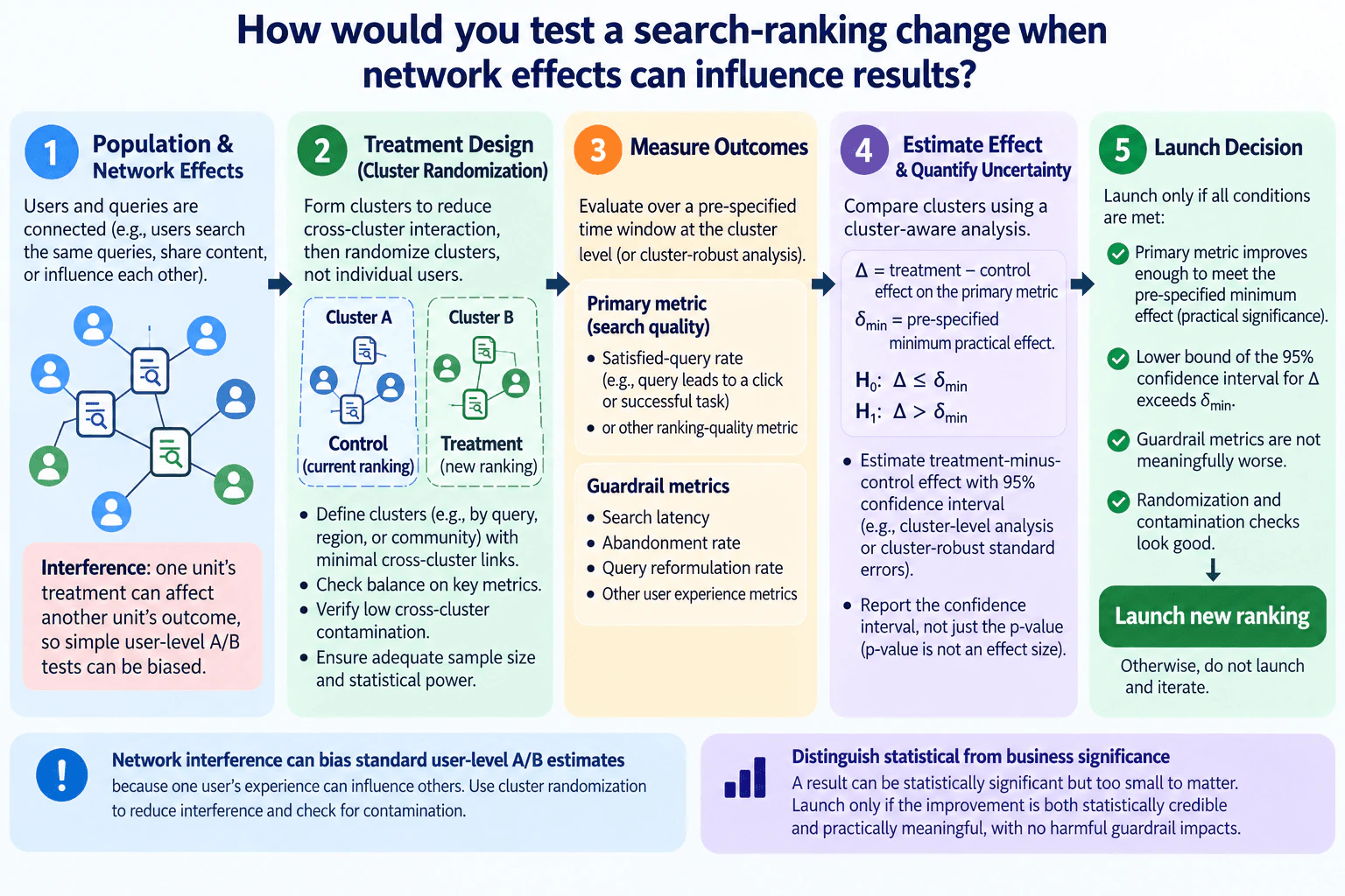
How would you test a search-ranking change when network effects can influence results? diagram
How to Explain It in an Interview
Test Setup
1. Define the population and interference risk

I would first define the eligible search population, the analysis grain, and a pre-specified experiment window. The key issue is interference: one experimental unit's treatment can affect another unit's outcome. For example, users may interact with the same queries or content, so treatment and control can influence each other. In that situation, a standard user-level A/B estimate can be biased.

2. Randomize clusters rather than individual users

I would create clusters with strong interaction inside each cluster and as little interaction as possible across clusters. Depending on how the network effect occurs, an appropriate clustering unit could be based on query, region, community, or another defensible grouping. I would then randomly assign entire clusters to control or treatment.

Control receives the current ranking and treatment receives the new ranking. Before reading any lift, I would verify balance on important pre-treatment characteristics and confirm that the design has enough clusters and observations for adequate statistical power.

Cluster randomization reduces interference, but it does not guarantee that interference disappears. I would therefore measure cross-cluster contamination and treat substantial remaining contamination as a validity risk.

3. Pre-specify the evaluation metrics

The primary metric should directly measure search quality. The diagram uses satisfied-query rate as an example, such as the share of queries that lead to a useful click or successful task under a pre-defined success rule. I would agree on the exact numerator and denominator before the test rather than defining them after seeing results.

I would also monitor guardrails for harmful side effects. The diagram includes search latency, abandonment rate, query reformulation rate, and other user-experience metrics. Their definitions and acceptable limits should also be specified before analyzing the experiment.

4. Define the estimand and hypotheses

Let Δ be the treatment-minus-control effect on the primary metric. Let δ_min be the pre-specified minimum practical effect required for launch.

The decision hypotheses are:

H0: Δ ≤ δ_min

H1: Δ > δ_min

This directly connects the statistical test to practical significance. A tiny positive effect is not enough merely because it is statistically detectable; the effect must be large enough to clear the launch threshold.

Statistical Checks
5. Estimate the effect with cluster-aware uncertainty

Because treatment is assigned at the cluster level, the analysis must respect clustering. I would estimate Δ using a cluster-level analysis or another appropriate method with cluster-robust standard errors. Treating every user-level observation as independent would generally understate uncertainty when observations inside the same cluster are correlated.

I would report the treatment-minus-control estimate with a 95% confidence interval. I would use the interval to communicate uncertainty and would not treat a p value as the magnitude of the effect.

6. Validate the experiment before trusting the result

Before making a launch decision, I would check:

  • Randomization balance between treatment and control clusters.
  • Whether the planned sample size and statistical power were achieved.
  • Cluster sizes and whether a few clusters dominate the estimate.
  • Missing data, attrition, logging changes, or exposure problems.
  • Cross-cluster contamination or spillovers.
  • Whether the primary and guardrail metrics used their pre-specified definitions.
  • Whether unplanned peeking or multiple testing could distort inference.

Selection bias or confounding can still enter if eligibility, exposure, logging, or analysis differs systematically between treatment and control. A narrow confidence interval around a biased estimate would still be misleading.

Result Meaning
7. Apply the launch rule

I would launch only if all required conditions pass:

  1. The primary metric improves enough to meet the pre-specified practical threshold.
  2. The lower bound of the 95% confidence interval for Δ exceeds δ_min.
  3. Guardrail metrics are not meaningfully worse according to their pre-defined limits.
  4. Randomization, data-quality, and contamination checks are acceptable.

If any condition fails, I would not launch from this experiment. I would investigate the failure, revise either the ranking change or the experimental design when appropriate, and test again.

8. Separate statistical significance from business significance

A result can be statistically credible but still too small to matter. The launch decision therefore needs both statistical evidence and practical significance. Conversely, a promising point estimate with a wide confidence interval is not enough because the evidence is still too uncertain to show that the practical threshold has been cleared.

9. Communicate the result at the strength the design supports

I would report the estimated effect, its 95% confidence interval, δ_min, guardrail behavior, and any remaining interference or measurement limitations. I would not claim that cluster randomization completely eliminates network effects. It reduces contamination when clusters are well designed, but meaningful cross-cluster interaction should remain an explicit limitation.

Technical Approach
  1. Define the eligible search population, analysis grain, primary metric, guardrails, fixed experiment window, and minimum practical effect δ_min before examining outcomes.
  2. Identify the mechanism of network interference and form clusters that minimize cross-cluster interaction.
  3. Randomly assign whole clusters to control using the current ranking or treatment using the new ranking.
  4. Check pre-treatment balance, cluster sizes, planned sample size, statistical power, and expected contamination before reading lift.
  5. Run the experiment for the pre-specified window and compute the primary and guardrail metrics using fixed definitions.
  6. Define Δ as the treatment-minus-control effect on the primary metric and evaluate H0: Δ ≤ δ_min against H1: Δ > δ_min.
  7. Estimate Δ using a cluster-aware analysis and report a 95% confidence interval.
  8. Validate randomization, missingness or attrition, metric logging, contamination, peeking, and any formal multiple-testing procedure.
  9. Launch only if the lower bound of the 95% confidence interval exceeds δ_min, guardrails are not meaningfully worse, and validity checks pass; otherwise do not launch and investigate.
Practical Insights

The main tradeoff is statistical efficiency. Cluster randomization usually creates fewer effectively independent experimental units than user-level randomization because observations inside a cluster can be correlated. That can require more traffic, more clusters, or a longer experiment to achieve the desired power. Larger clusters may reduce contamination between treatment and control but leave fewer randomized units. Smaller clusters provide more randomized units but may allow more spillover. The analysis is also more complex because uncertainty must account for clustering and the team must monitor contamination in addition to ordinary metric lift.

Why Interviewers Ask This

This tests whether the candidate recognizes that network interference can bias a standard user-level A/B estimate, chooses a treatment design that reduces contamination, defines appropriate primary and guardrail metrics, quantifies uncertainty at the correct experimental level, and separates statistical evidence from the practical improvement required for launch.

Common interview mistakes

Common mistakes include randomizing individual users even when treatment can spill across users; choosing clusters without checking cross-cluster interaction; reading lift before checking randomization balance, sample size, and power; treating correlated observations inside a cluster as independent; using a p value as an effect size; declaring success merely because an effect is above zero when it does not clear the practical threshold; changing the primary metric, threshold, or stopping rule after seeing results; ignoring latency, abandonment, reformulation, or other guardrails; overlooking contamination, attrition, selection bias, confounding, peeking, and multiple testing; and making a causal claim stronger than the experiment design supports.

Interview tip

Organize the answer as treatment design, metrics, statistical analysis, and launch rule. Start with interference as the reason a simple user-level A/B test may be biased. Then explain cluster randomization, one primary search-quality metric plus guardrails, cluster-aware confidence intervals, and the minimum practical effect. Finish with the exact rule: launch only when the 95% confidence interval's lower bound exceeds δ_min, guardrails remain acceptable, and randomization and contamination checks pass.

Interviewer may ask next
What would you do if treatment and control clusters still had substantial interaction?

I would not assume the cluster design has solved interference. I would quantify cross-cluster contamination and determine whether it is large enough to bias the estimand. If it is material, I would redesign the clusters so more interacting units stay together, change the experiment scope, or use another interference-aware design that better matches how exposure propagates. I would then recalculate power because changing cluster size or the number of clusters changes the effective sample size. If substantial interference remains, I would report it as a limitation and avoid interpreting the result as an uncontaminated treatment effect.

What if the new ranking is statistically better than control but the effect does not clear the minimum practical threshold?

I would not launch under the stated decision rule. Evidence that Δ is above zero is not enough because the launch criterion requires an improvement larger than δ_min. If the lower bound of the 95% confidence interval does not exceed δ_min, the experiment has not demonstrated that the ranking change clears the practical threshold. I would report the point estimate and confidence interval, confirm the guardrails and validity checks, and either stop, continue only under a pre-specified design that allows more data, or improve the ranking before testing again.

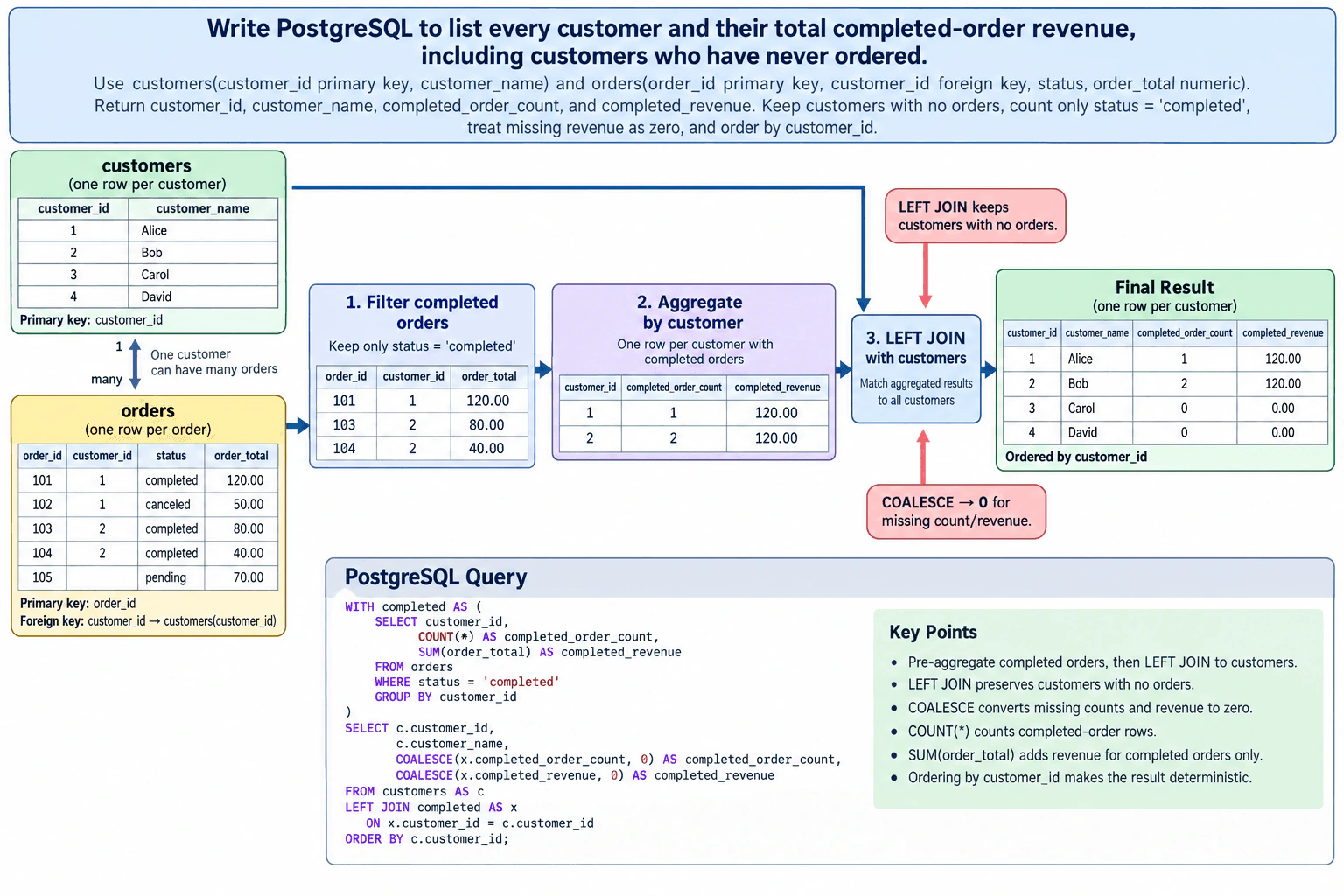
45. Write PostgreSQL to list every customer and their total completed-order revenue, including customers who have never ordered.Sql And DatabasesEasy

Question Details

Use customers(customer_id primary key, customer_name) and orders(order_id primary key, customer_id foreign key, status, order_total numeric). Return customer_id, customer_name, completed_order_count, and completed_revenue. Keep customers with no orders, count only status = 'completed', treat missing revenue as zero, and order by customer_id.

Short Interview Answer (30-60 seconds)

I would first aggregate only completed orders to one row per customer, then LEFT JOIN that result to customers. The LEFT JOIN keeps customers even when they have no matching orders. In the CTE, COUNT() gives the number of completed orders and SUM(order_total) gives completed revenue. After the join, customers without completed orders have NULL aggregate values, so I use COALESCE to return zero. Finally, I order the output by customer_id.

Detailed Explanation

See the Code while reading this explanation.

The goal is to return exactly one row for every customer, even when that customer has never ordered or has no completed orders. The customers table has one row per customer because customer_id is its primary key, while orders has one row per order and can contain many rows for the same customer. I first keep only completed orders and aggregate them to one row per customer. Then I LEFT JOIN those totals back to customers. This preserves the full customer population and avoids multiple final rows per customer. COALESCE turns missing aggregate values into zero, and ORDER BY customer_id gives the requested ordering.

Useful Questions to Ask the Interviewer
  1. Should only the exact status value 'completed' count, or are there other statuses that represent a completed order?
  2. Can order_total be NULL for a completed order, and if so, should that amount be treated as zero or flagged as a data-quality issue?
  3. Should the result remain one row per customer even when different customers have the same customer_name?
Write PostgreSQL to list every customer and their total completed-order revenue, including customers who have never ordered. diagram
How to Explain It in an Interview

Start with the grain. The customers table has one row per customer, identified by the customer_id primary key. The orders table has one row per order, so one customer can have many order rows through orders.customer_id. The required output grain is one row per customer.

The query follows the same flow as the diagram: filter completed orders, aggregate them by customer, then LEFT JOIN those aggregates to the complete customer list.

First, the completed CTE filters orders with WHERE status = 'completed'. That means pending, cancelled, and other statuses do not contribute to either the count or the revenue. GROUP BY customer_id then reduces those completed-order rows to one row per customer. COUNT() calculates completed_order_count, and SUM(order_total) calculates completed_revenue.

Next, the outer query starts from customers and LEFT JOINs the completed aggregate on customer_id. LEFT JOIN is the important choice because it keeps every row from customers, including customers with no orders and customers whose orders exist but none are completed. An INNER JOIN would incorrectly remove those customers.

Because the CTE already has at most one row per customer_id, joining it to customers does not multiply the final customer rows. For a customer with no matching completed aggregate, completed_order_count and completed_revenue are NULL after the join. COALESCE(x.completed_order_count, 0) and COALESCE(x.completed_revenue, 0) convert those missing values to the required zeros.

Finally, ORDER BY c.customer_id returns the output in customer_id order.

For validation, I would check that the result row count equals the row count of customers and that customer_id is unique in the result. I would also compare the sum of completed_order_count with a separate count of orders where status = 'completed', and compare total completed_revenue with a separate control sum over completed orders. If completed orders can contain NULL order_total values, I would inspect those separately because SUM ignores NULL inputs; whether a NULL amount should represent zero is a business and data-quality decision.

Technical Approach
  1. Confirm the grain: customers is one row per customer and orders is one row per order.
  2. Filter orders to status = 'completed'.
  3. GROUP BY customer_id and calculate COUNT() as completed_order_count and SUM(order_total) as completed_revenue.
  4. LEFT JOIN the one-row-per-customer aggregate to customers using customer_id.
  5. Use COALESCE to convert missing completed_order_count and completed_revenue values to zero.
  6. Return customer_id, customer_name, completed_order_count, and completed_revenue.
  7. ORDER BY customer_id.
  8. Validate customer row count, uniqueness, completed-order counts, and revenue control totals.
Practical Complexity & Trade-offs

The database must scan the relevant order rows, group completed orders by customer_id, and join those grouped rows to customers. The amount of work grows with the number of customers and orders. Pre-aggregating completed orders before the LEFT JOIN keeps the joined aggregate at one row per customer instead of carrying every order row into the final result. Actual speed depends on table size, data distribution, indexes, and the PostgreSQL execution plan, so no specific runtime should be assumed.

Example

The implementation uses a CTE to filter and pre-aggregate completed orders by customer_id. The outer query LEFT JOINs those per-customer aggregates to customers, applies COALESCE for customers with no matching completed orders, and orders the result by customer_id. This keeps the final grain at exactly one row per customer and matches the diagram's filter → aggregate → LEFT JOIN → zero-fill flow.

Code
WITH
  completed AS (
    SELECT
      customer_id,
      COUNT() AS completed_order_count,
      SUM(order_total) AS completed_revenue
    FROM
      orders
    WHERE
      status = 'completed'
    GROUP BY
      customer_id
  )
SELECT
  c.customer_id,
  c.customer_name,
  COALESCE(x.completed_order_count, 0) AS completed_order_count,
  COALESCE(x.completed_revenue, 0) AS completed_revenue
FROM
  customers AS c
  LEFT JOIN completed AS x ON x.customer_id = c.customer_id
ORDER BY
  c.customer_id;
Where it is used

This pattern is common in customer revenue reports, account summaries, operational dashboards, and other analysis where entities with zero related activity must still appear. The same approach can be used for products with no sales, employees with no assignments, or accounts with no qualifying transactions.

Why Interviewers Ask This

This tests whether the candidate understands table grain, one-to-many relationships, filtering before aggregation, LEFT JOIN behavior, aggregate functions, NULL handling, and deterministic ordering. The key judgment is preserving every customer while counting and summing only completed orders without multiplying customer rows.

Common interview mistakes

Using INNER JOIN and dropping customers with no completed orders; filtering status = 'completed' in a WHERE clause after a LEFT JOIN to raw orders and thereby removing unmatched customers; joining raw orders without grouping and producing multiple rows per customer; counting all statuses instead of completed orders only; forgetting COALESCE and returning NULL instead of zero; grouping at the wrong grain; or omitting the required ORDER BY customer_id.

Interview tip

Explain the grain before writing the SQL: orders starts at one row per order, the CTE reduces completed orders to one row per customer, and the LEFT JOIN preserves every customer. Then call out COALESCE because handling customers with no matching completed orders is the key edge case.

Interviewer may ask next
What would you check if completed orders can have a NULL order_total?

COUNT() would still count that completed order, while SUM(order_total) ignores NULL values. I would first confirm the business rule for a missing amount instead of automatically treating an actual NULL order_total as zero. I would inspect completed rows where order_total IS NULL and either keep the current behavior, substitute zero at the row level if that is the approved rule, or flag those rows as a data-quality problem.

How would the approach change if the orders table were very large?

I would keep the same correctness-first query shape and inspect PostgreSQL's execution plan before changing it. Pre-aggregating completed orders before the join already reduces the joined data to one row per customer. If performance is still a problem, I would evaluate the actual filter, aggregation, and join costs and then consider indexing or other physical-design changes based on the workload and data distribution rather than assuming one specific optimization is always best.

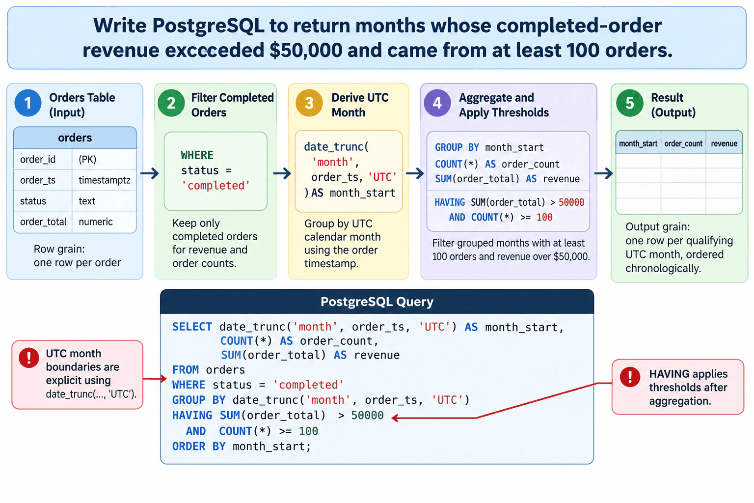
46. Write PostgreSQL to return months whose completed-order revenue exceeded $50,000 and came from at least 100 orders.Sql And DatabasesEasy

Question Details

Use orders(order_id primary key, order_ts timestamptz, status, order_total numeric). Return month_start, order_count, and revenue for status = 'completed'. Group in UTC calendar months, filter groups with HAVING, and order chronologically.

Short Interview Answer (30-60 seconds)

I would first filter to status = 'completed'. Then I would derive the UTC month start from order_ts, group by that month, count the completed orders, and sum order_total as revenue. The aggregate thresholds belong in HAVING: revenue must be greater than 50,000 and the order count must be at least 100. Finally, I would order by month_start so the qualifying UTC months are returned chronologically.

Detailed Explanation

Each row in orders represents one order because order_id is the primary key. The query first keeps only rows whose status is 'completed'. It then converts each order_ts into the start of its UTC calendar month. After grouping at that monthly grain, COUNT() returns the completed-order count and SUM(order_total) returns revenue. HAVING keeps only months with revenue greater than $50,000 and at least 100 orders. ORDER BY month_start finally returns the qualifying months in chronological order, with one output row per UTC month.

Useful Questions to Ask the Interviewer
  1. Can order_ts or order_total be NULL for completed orders?
  2. Should COUNT() include a completed order when its order_total is NULL?
  3. Is order_total already the exact revenue amount to sum, with no additional refund, tax, or currency rules?
Write PostgreSQL to return months whose completed-order revenue exceeded $50,000 and came from at least 100 orders. diagram
How to Explain It in an Interview

The input grain is one row per order. order_id is the primary key, and the query uses only the orders table, so no join is needed and there is no join-driven row multiplication.

First, WHERE status = 'completed' filters individual rows before aggregation. A NULL status does not satisfy this equality condition, so it is not treated as completed.

Next, date_trunc('month', order_ts, 'UTC') places each timestamptz value into its UTC calendar-month bucket and returns that bucket start as month_start. Explicitly using UTC is important because calendar-month boundaries can differ by time zone.

GROUP BY changes the grain from one row per order to one row per UTC month. COUNT() gives the number of completed-order rows in each month. SUM(order_total) gives monthly completed-order revenue.

HAVING is used for the thresholds because the conditions depend on aggregate values that exist only after grouping. The revenue rule is strictly greater than 50000, while the order-count rule is greater than or equal to 100, matching the question exactly.

Finally, ORDER BY month_start returns the qualifying months in chronological order.

For NULL handling, COUNT() still counts a completed-order row even if order_total is NULL. SUM(order_total) ignores individual NULL values; if every order_total in a month were NULL, SUM would be NULL and that month would not satisfy SUM(order_total) > 50000. A NULL order_ts produces a NULL month_start group, so I would confirm whether such rows can exist and whether they should be excluded rather than silently changing the requirement.

I would validate the query by comparing completed-order row counts and revenue totals for selected UTC months against an independent trusted control using the same status filter and UTC month boundaries.

The complete PostgreSQL is:

SELECT date_trunc('month', order_ts, 'UTC') AS month_start, COUNT() AS order_count, SUM(order_total) AS revenue FROM orders WHERE status = 'completed' GROUP BY date_trunc('month', order_ts, 'UTC') HAVING SUM(order_total) > 50000 AND COUNT() >= 100 ORDER BY month_start;

Technical Approach
  1. Start from orders at one row per order.
  2. Filter to status = 'completed'.
  3. Derive month_start with date_trunc('month', order_ts, 'UTC').
  4. Group by that UTC month.
  5. Compute COUNT() as order_count and SUM(order_total) as revenue.
  6. Use HAVING to keep groups where revenue > 50000 and order_count >= 100.
  7. Order by month_start chronologically.
  8. Validate selected monthly counts and revenue against a trusted control using the same UTC boundaries.
Practical Complexity & Trade-offs

The main work is reading the relevant orders and aggregating them by month. If n rows are scanned and g monthly groups are produced, filtering and aggregation are roughly O(n), while ordering the monthly results is roughly O(g log g). The grouping state is roughly O(g). In practice, actual PostgreSQL cost depends on the execution plan, table size, data distribution, and available indexes.

Where it is used

This pattern is common in monthly finance, sales, and operations reporting when analysts need to identify periods that satisfy both a revenue threshold and a minimum transaction-volume requirement while keeping time boundaries consistent.

Why Interviewers Ask This

The interviewer is checking whether I can preserve the order-level input grain, filter rows before aggregation, group timestamptz values into the requested UTC calendar months, calculate order count and revenue correctly, use HAVING for aggregate conditions, and return the qualifying months in chronological order without adding unnecessary joins or logic.

Common interview mistakes

Common mistakes are placing SUM or COUNT conditions in WHERE instead of HAVING, grouping by the session time zone instead of explicitly using UTC, using >= 50000 instead of the required > 50000, using > 100 instead of the required >= 100, counting a nullable revenue column instead of order rows, forgetting ORDER BY month_start, adding an unnecessary join that can multiply rows, or inventing result values that were not supplied.

Interview tip

State the grain first: one input row per order and one output row per qualifying UTC month. Then explain the flow as WHERE filters rows, date_trunc defines the UTC month, GROUP BY changes the grain, aggregate functions calculate the metrics, HAVING filters groups, and ORDER BY makes the result chronological.

Interviewer may ask next
What would you check if order_ts or order_total can be NULL?

A NULL status does not pass status = 'completed'. A NULL order_ts produces a NULL month_start group, so I would confirm whether those rows should be excluded. COUNT() still counts a completed row when order_total is NULL, while SUM(order_total) ignores that NULL value. If every order_total in a month is NULL, SUM returns NULL and the month does not pass the revenue condition. I would confirm that this matches the intended business rules before changing the query.

How would the query change if months had to follow a business time zone instead of UTC?

I would keep the same row filter, monthly aggregation, HAVING thresholds, and chronological ordering, but replace 'UTC' in date_trunc with the required business time zone. This matters for orders near month boundaries because the same instant can fall in different calendar months in different time zones. I would then validate timestamps around the beginning and end of a month in that zone.

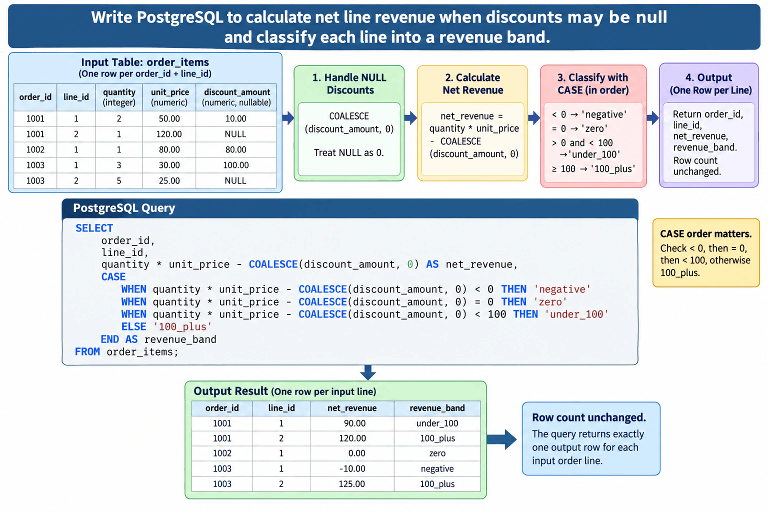
47. Write PostgreSQL to calculate net line revenue when discounts may be null and classify each line into a revenue band.Sql And DatabasesEasy

Question Details

Use order_items(order_id, line_id, quantity integer, unit_price numeric, discount_amount numeric null). Return order_id, line_id, net_revenue = quantity * unit_price - discount_amount with null discount treated as zero, and a CASE band of negative, zero, under_100, or 100_plus. Preserve one output row per input line.

Short Interview Answer (30-60 seconds)

I would keep the query at one row per order line, replace a NULL discount with zero using COALESCE, calculate net_revenue as quantity * unit_price - COALESCE(discount_amount, 0), and classify that result with CASE. I would check negative first, then zero, then values below 100, with everything else classified as 100_plus. Because there is no join, aggregation, or filter, every input line produces exactly one output row.

Detailed Explanation

See the Code while reading this explanation.

The task is to calculate revenue separately for every row in order_items without changing the table's grain. Each input row represents one order line identified by order_id and line_id. A missing discount must behave like zero, because subtracting NULL directly would produce NULL instead of a usable revenue value. After calculating net_revenue, the query assigns exactly one label based on its value: negative, zero, under_100, or 100_plus. No join, grouping, filtering, or window function is needed, so the output stays one row per input line.

Useful Questions to Ask the Interviewer
  1. Should a NULL discount always mean no discount, or can it mean unknown data?
  2. Are quantity and unit_price guaranteed to be non-NULL and valid for every line?
  3. Should exactly 100 belong to 100_plus, as specified?
  4. Is (order_id, line_id) expected to identify one unique input line?
Write PostgreSQL to calculate net line revenue when discounts may be null and classify each line into a revenue band. diagram
How to Explain It in an Interview

Start with the grain: the input is already at one row per order line, and the required output has the same grain. There is no need to join, aggregate, group, rank, or deduplicate rows.

First, handle the nullable discount. In PostgreSQL, arithmetic with a NULL operand produces NULL, so subtracting discount_amount directly can make net_revenue NULL. Use COALESCE(discount_amount, 0) to substitute zero when discount_amount is NULL.

The row-level calculation is: net_revenue = quantity * unit_price - COALESCE(discount_amount, 0)

Next, classify that same value with an ordered CASE expression. The boundaries match the requested bands exactly:

  • net_revenue < 0 -> negative
  • net_revenue = 0 -> zero
  • net_revenue > 0 and net_revenue < 100 -> under_100
  • net_revenue >= 100 -> 100_plus

The CASE order matters. After checking negative and zero, a remaining value below 100 must be positive, so the third WHEN can simply test net_revenue < 100. The ELSE branch then covers values of 100 or more.

A direct PostgreSQL solution is:

SELECT order_id, line_id, quantity * unit_price - COALESCE(discount_amount, 0) AS net_revenue, CASE WHEN quantity * unit_price - COALESCE(discount_amount, 0) < 0 THEN 'negative' WHEN quantity * unit_price - COALESCE(discount_amount, 0) = 0 THEN 'zero' WHEN quantity * unit_price - COALESCE(discount_amount, 0) < 100 THEN 'under_100' ELSE '100_plus' END AS revenue_band FROM order_items;

This matches the approved diagram's flow: handle NULL discounts, calculate net revenue, classify with CASE, and return one row per input line. The diagram's examples are also consistent with the logic: 90 is under_100, 120 is 100_plus, 0 is zero, -10 is negative, and 125 is 100_plus.

For validation, compare the input row count with the output row count; they should be identical because the query performs only row-level expressions and does not filter or join. Also test the important boundaries: a NULL discount, a negative result, exactly zero, a value just below 100, and exactly 100. If NULL means 'unknown discount' instead of 'no discount,' then replacing it with zero would change the meaning of the data, so that business rule should be confirmed.

Technical Approach
  1. Keep the input grain at one row per order line identified by order_id and line_id.
  2. Replace NULL discount_amount with 0 using COALESCE.
  3. Calculate net_revenue as quantity * unit_price - COALESCE(discount_amount, 0).
  4. Classify net_revenue in order: values below 0 as negative, exactly 0 as zero, values below 100 as under_100, and all remaining values as 100_plus.
  5. Return order_id, line_id, net_revenue, and revenue_band without joins, aggregation, or filtering.
  6. Validate that the output row count equals the input row count and test all classification boundaries.
Practical Complexity & Trade-offs

The query performs a constant amount of arithmetic and comparison work for each input row, so the row-processing work grows roughly in proportion to the number of order_items rows. It does not require a join, grouping, sorting, or window function. The direct version repeats the net-revenue expression inside CASE, which is simple for this short calculation; a subquery can calculate it once if the expression becomes longer or harder to maintain.

Example

A subquery can calculate net_revenue once and let the outer SELECT classify that value. This avoids repeating the arithmetic while preserving the same one-row-per-input-line grain and the same band boundaries.

Code
SELECT
  order_id,
  line_id,
  net_revenue,
  CASE
    WHEN net_revenue < 0 THEN 'negative'
    WHEN net_revenue = 0 THEN 'zero'
    WHEN net_revenue < 100 THEN 'under_100'
    ELSE '100_plus'
  END AS revenue_band
FROM
  (
    SELECT
      order_id,
      line_id,
      quantity * unit_price - COALESCE(discount_amount, 0) AS net_revenue
    FROM
      order_items
  ) AS line_revenue;
Where it is used

This pattern is common in order-line reporting, invoice analysis, transaction detail reports, revenue checks, and data-quality workflows where an analyst needs a calculated amount and a category while preserving one output row per source line.

Why Interviewers Ask This

This tests whether you can write correct row-level PostgreSQL, handle NULL values safely, preserve the required data grain, calculate a derived numeric value, and use an ordered CASE expression with exact boundary conditions.

Common interview mistakes

Common mistakes are subtracting discount_amount without COALESCE and producing NULL net revenue; checking only net_revenue < 100 before handling negative and zero values; using <= 100 and incorrectly putting exactly 100 into under_100; classifying gross revenue instead of net revenue; adding GROUP BY or DISTINCT even though the required grain is already one row per input line; or adding an unnecessary join that could multiply rows.

Interview tip

State the row grain and NULL rule first, then walk through the CASE boundaries in order. Call out that exactly 100 belongs to 100_plus, and finish by saying you would verify that the output row count matches the input row count.

Interviewer may ask next
What would you change if NULL discount_amount meant 'discount unknown' instead of 'no discount'?

I would not automatically replace NULL with zero, because that would convert missing information into a known zero discount. I would first confirm the required business rule. If NULL must remain unknown, net_revenue could remain NULL or the output could use a separate status if the specification allows it. COALESCE(discount_amount, 0) is correct only when NULL is explicitly defined to mean no discount.

What would you change if the revenue calculation became more complex and you wanted to avoid repeating it inside CASE?

I would calculate net_revenue once in a subquery or CTE and classify it in the outer SELECT. That gives the calculation one definition, reduces duplication, and keeps the same one-row-per-input-line result. For this short expression, the direct query remains simple and correct, while the subquery approach is easier to maintain as the calculation grows.

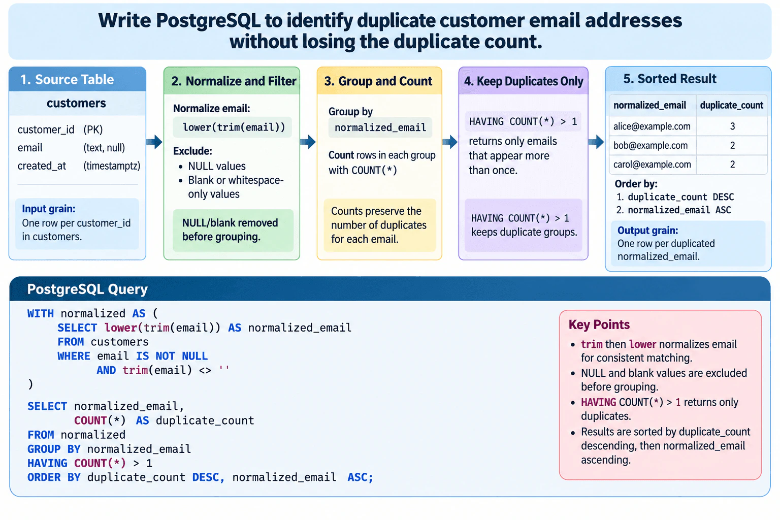
48. Write PostgreSQL to identify duplicate customer email addresses without losing the duplicate count.Sql And DatabasesEasy

Question Details

Use customers(customer_id primary key, email text null, created_at timestamptz). Normalize email with trim and lower, exclude null and blank values, and return normalized_email and duplicate_count only where the count exceeds one. Sort by duplicate_count descending and normalized_email ascending.

Short Interview Answer (30-60 seconds)

I would normalize each usable email with lower(trim(email)), excluding NULL and blank values first. Then I would group by the normalized email and use COUNT() to preserve how many customer rows belong to each group. HAVING COUNT() > 1 keeps only duplicate groups. Finally, I would return normalized_email and duplicate_count, sorted by duplicate_count descending and normalized_email ascending. A CTE makes the normalization and filtering step explicit before aggregation.

Detailed Explanation

See the Code while reading this explanation.

The task is to find email addresses that belong to more than one customer after ignoring differences in letter case and surrounding spaces. The input grain is one row per customer_id in customers because customer_id is the primary key. First, exclude rows where email is NULL or becomes blank after trimming. Then normalize each remaining email with lower(trim(email)). Group those normalized values and count the customer rows in each group. Keep only groups with a count greater than one. The final grain is one row per duplicated normalized email, with its duplicate count, sorted exactly as requested.

Useful Questions to Ask the Interviewer
  1. Should case and leading or trailing spaces be the only email differences treated as equivalent?
  2. Should NULL and whitespace-only email values be excluded completely? The requirement says yes.
  3. Is the duplicate definition based on all customer rows regardless of created_at? The requirement provides no date filter, so this query uses all rows.
  4. Do you want only the grouped duplicate summary, or also the individual customer_id values? This question asks only for normalized_email and duplicate_count.
Write PostgreSQL to identify duplicate customer email addresses without losing the duplicate count. diagram
How to Explain It in an Interview

The customers table has one row per customer_id because customer_id is the primary key. There is no JOIN in this solution, so there is no risk of multiplying rows through a one-to-many relationship.

The first step is normalization. Here, normalization means converting email text into the comparison form required by the question. lower(trim(email)) removes surrounding spaces and converts letters to lowercase. Values that differ only by surrounding whitespace or letter case therefore fall into the same group. This is intentionally limited to the normalization rule given in the question; it does not add provider-specific email rewriting rules.

Before grouping, the query excludes email IS NULL. In SQL, NULL represents an unknown or missing value, and comparisons involving NULL do not evaluate to TRUE. Handling it explicitly makes the intended population clear. The condition trim(email) <> '' also removes empty strings and whitespace-only strings before they can become a meaningless grouped value.

The CTE named normalized produces one normalized_email value for every valid customer row. The outer query then changes the grain from one row per customer to one row per normalized email by using GROUP BY normalized_email.

COUNT() preserves the number of customer rows in each normalized-email group. HAVING COUNT() > 1 is used because the duplicate condition applies after aggregation. WHERE filters source rows before grouping, while HAVING filters the grouped result after COUNT() has been calculated.

The final SELECT returns only normalized_email and COUNT() AS duplicate_count, matching the requested output. ORDER BY duplicate_count DESC places the largest duplicate groups first. normalized_email ASC provides the required secondary ordering when two groups have the same duplicate count.

A concrete validation is to select a returned normalized_email and count matching source rows using the same lower(trim(email)) expression and the same NULL and blank filters. That source count should equal duplicate_count. I would also confirm that every returned duplicate_count is greater than one and that no NULL or blank normalized_email appears.

created_at is not used because the question specifies no date boundary. Adding a created_at filter would change the population and could change duplicate counts, so I would not introduce one without an explicit requirement.

The main tradeoff is the definition of normalization. lower(trim(email)) is exactly what the question asks for and is easy to explain, but it does not guarantee that every address pointing to the same real mailbox will be merged. More aggressive canonicalization would require additional business rules and could incorrectly combine distinct addresses.

Technical Approach
  1. Start from customers at one row per customer_id.
  2. Exclude rows where email IS NULL.
  3. Exclude blank or whitespace-only emails with trim(email) <> ''.
  4. Normalize each remaining email with lower(trim(email)).
  5. Group rows by normalized_email.
  6. Count rows in each group with COUNT().
  7. Keep only groups where COUNT() > 1 using HAVING.
  8. Return normalized_email and duplicate_count.
  9. Sort by duplicate_count DESC, then normalized_email ASC.
  10. Validate selected groups against the source rows using the same normalization and filtering rules.
Practical Complexity & Trade-offs

PostgreSQL must read the qualifying customer rows and group them by normalized email. For n source rows, the scan work grows with n. The exact grouping cost depends on the execution plan, such as hash aggregation or sorting, so it should not be described as one guaranteed complexity. If d duplicate groups are returned, the final requested ordering sorts those d groups, which is conceptually about d log d work. Correctness comes first; indexing or other optimization should be considered only after checking the real data size and query plan.

Example

Use a CTE to normalize and filter source rows once. Then aggregate by normalized_email, preserve each group's size with COUNT(), keep only groups whose count exceeds one with HAVING, and apply the required ordering.

Code
WITH
  normalized AS (
    SELECT
      lower(trim(email)) AS normalized_email
    FROM
      customers
    WHERE
      email IS NOT NULL
      AND trim(email) <> ''
  )
SELECT
  normalized_email,
  COUNT() AS duplicate_count
FROM
  normalized
GROUP BY
  normalized_email
HAVING
  COUNT() > 1
ORDER BY
  duplicate_count DESC,
  normalized_email ASC;
Where it is used

This pattern is useful for customer-data cleanup, CRM deduplication, account-quality checks, mailing-list audits, migration validation, and reports that need both the duplicated value and the number of source records sharing it.

Why Interviewers Ask This

This checks whether the candidate can normalize messy text, handle NULL and blank values correctly, aggregate at the right grain, preserve the duplicate count, filter aggregate groups with HAVING, and produce deterministic ordered output in PostgreSQL.

Common interview mistakes

Common mistakes are grouping by the original email instead of the normalized value; using DISTINCT and losing the duplicate count; counting before applying the required normalization; allowing NULL, empty, or whitespace-only emails into the groups; putting COUNT() > 1 in WHERE instead of HAVING; returning customer-level rows when the required output grain is one row per duplicated normalized email; adding an unsupported created_at filter; or forgetting the secondary normalized_email ascending sort.

Interview tip

State the grains first: one row per customer in the input and one row per duplicated normalized email in the output. Then explain the query in four steps: normalize, filter, group and count, then keep duplicates. Mention that HAVING is required because the duplicate condition is evaluated after aggregation.

Interviewer may ask next
What if the interviewer asks you to verify that a reported duplicate_count is correct?

Take a returned normalized_email and query customers again using the same lower(trim(email)) expression while applying the same NULL and blank filters. Count those matching customer rows and compare that count with duplicate_count. I would also confirm that every final group has a count greater than one and that no NULL or blank normalized value appears.

What changes if the business later wants duplicates only among customers created during a specific period?

Add an explicit created_at boundary to the source-row filter before aggregation because the date condition changes which customer rows contribute to each count. Since created_at is timestamptz, the intended time zone and interval boundaries should be defined. A half-open range such as created_at >= start_time AND created_at < end_time avoids overlap between adjacent reporting periods.

49. Write PostgreSQL to summarize completed revenue by week for the previous eight complete weeks.Sql And DatabasesEasy

Question Details

Use orders(order_id primary key, order_ts timestamptz, status, order_total numeric). Weeks start Monday in UTC. Exclude the current partial week, return week_start, order_count, and revenue, include only completed orders, and order oldest to newest.

Short Interview Answer (30-60 seconds)

I would find the start of the current UTC week and use it as the exclusive upper boundary. The lower boundary is exactly eight weeks earlier. Then I would keep only completed orders in that half-open range, group them by Monday UTC week_start, count the orders, sum order_total as revenue, and sort by week_start ascending. No JOIN is needed because all required fields are already in orders.

Detailed Explanation

The source table has one row per order, identified by the primary key order_id. The task is to turn those order-level rows into weekly totals for the previous eight complete UTC weeks. I first calculate the Monday start of the current UTC week and exclude everything from that boundary forward, so the current partial week is not included. I then go back eight weeks for the inclusive lower boundary. After filtering to completed orders, I group by UTC week start, count rows for order_count, sum order_total for revenue, and sort from oldest to newest.

Useful Questions to Ask the Interviewer
  1. Should weeks with zero completed orders appear as rows with zero values, or should the query return only weeks that have completed orders?
  2. Can order_total be NULL, and if so, should NULL amounts be ignored by SUM or treated as zero?
  3. Is the exact status value always lowercase 'completed'?
Write PostgreSQL to summarize completed revenue by week for the previous eight complete weeks. diagram
How to Explain It in an Interview

The input grain is one row per order. All required columns are already in orders, so there is no JOIN. That means there is also no one-to-many join that could multiply rows before aggregation.

The first important step is defining the UTC week boundary. The query uses date_trunc('week', ..., 'UTC') so the weekly bucket follows Monday-starting UTC weeks.

The current UTC week start is the exclusive upper bound:

order_ts < date_trunc('week', current_timestamp, 'UTC')

This removes every order in the current partial week.

The inclusive lower bound is eight weeks earlier:

order_ts >= date_trunc('week', current_timestamp, 'UTC') - interval '8 weeks'

Together, these predicates create the half-open interval [current_week_start - 8 weeks, current_week_start). That covers the previous eight complete Monday-to-Monday UTC weeks and avoids double-counting a boundary timestamp.

The status predicate keeps only completed orders:

status = 'completed'

If status is NULL, that row does not pass the predicate because a comparison with NULL is not true. A NULL order_ts also does not pass the date-range comparisons.

For the remaining rows, date_trunc('week', order_ts, 'UTC') produces week_start. GROUP BY 1 changes the grain from one row per order to one row per non-empty week. COUNT() becomes order_count, and SUM(order_total) becomes revenue. SUM ignores NULL order_total values; if all order_total values in a group are NULL, the revenue result for that group is NULL, so the business rule for NULL amounts should be confirmed if that case is possible.

ORDER BY 1 sorts week_start ascending, giving the requested oldest-to-newest order. Because there is only one grouped row for each week_start, there is no tie-ordering problem.

A useful validation is to run a control query with the same status and time filters but without GROUP BY, then compare its total COUNT() and SUM(order_total) with the sums of the grouped result. I would also test an order exactly at the lower boundary, an order exactly at the current-week boundary, and orders around a Monday UTC transition.

This query returns only weeks that contain at least one completed order, which matches the diagram's one-row-per-week-with-completed-orders result. If the requirement changes to always return all eight calendar weeks, including empty weeks, I would generate the eight week_start values and LEFT JOIN the weekly aggregates onto them.

Technical Approach
  1. Confirm the source grain is one row per order and that no JOIN is required.
  2. Compute the Monday start of the current week in UTC.
  3. Set the inclusive lower boundary to current UTC week start minus eight weeks.
  4. Set the exclusive upper boundary to the current UTC week start.
  5. Filter to status = 'completed' and order_ts inside that half-open range.
  6. Group by date_trunc('week', order_ts, 'UTC').
  7. Calculate COUNT() as order_count and SUM(order_total) as revenue.
  8. Sort by week_start ascending.
  9. Validate grouped counts and revenue against an ungrouped control query using the same filters.
Practical Complexity & Trade-offs

PostgreSQL filters the relevant order rows and then groups the matches into weekly buckets. If N rows are examined, the main work grows with the number of rows that must be scanned, while the aggregation itself needs only a small number of week groups. The output has at most eight non-empty weekly rows. Performance can improve with suitable indexing on a large table, but the query's correctness does not depend on assuming any specific index.

Where it is used

This pattern is common in weekly revenue reporting, finance summaries, sales dashboards, operational KPI reports, and scheduled analytics jobs where only fully completed reporting periods should be compared.

Why Interviewers Ask This

The interviewer is checking whether you can translate a reporting requirement into correct PostgreSQL while preserving row grain, UTC week boundaries, filtering, aggregation, and ordering. The key judgment is whether you exclude the current partial week and select exactly the previous eight complete Monday-to-Monday UTC weeks without adding unnecessary joins or changing the one-row-per-order source grain before aggregation.

Common interview mistakes

Common mistakes are including the current partial week, using the session time zone instead of explicit UTC week boundaries, subtracting eight weeks from the current timestamp instead of from the current week start, using an inclusive upper boundary, forgetting status = 'completed', grouping with a different time-zone rule from the filter, assuming the query always returns eight rows when an empty week has no matching orders, and assuming SUM(order_total) converts NULL values to zero.

Interview tip

Explain the query in the same order as the diagram: start with one row per order and no JOIN, filter to completed orders, restrict the data to the eight complete UTC weeks using an inclusive lower and exclusive upper boundary, group by Monday week_start, aggregate count and revenue, then sort oldest to newest.

Interviewer may ask next
What happens if one of the eight weeks has no completed orders?

This query returns no row for that week because GROUP BY can only create a group when matching rows exist. If the requirement is to always show all eight weeks, I would generate the eight Monday UTC week_start values, aggregate orders separately, LEFT JOIN the aggregates onto those weeks, and use COALESCE where the business rule calls for zero counts or revenue.

How would the query change if weeks should use a business time zone instead of UTC?

I would replace 'UTC' consistently with the required named business time zone when computing both the current-week boundaries and each order's week_start. Filtering and grouping must use the same time-zone definition so an order near a week boundary cannot be filtered according to one week definition and grouped according to another.

50. When combining current and archived customer leads, when should a Data Analyst use UNION instead of UNION ALL?Sql And DatabasesEasy

Question Details

Compare UNION and UNION ALL using current_leads(email, source, captured_at) and archived_leads(email, source, captured_at). Explain duplicate behavior and performance, then write PostgreSQL that preserves every source record and a second query that returns unique normalized email addresses.

Short Interview Answer (30-60 seconds)

I would use UNION only when duplicate output rows should be collapsed. UNION compares the complete selected rows, so two lead rows are duplicates only when all selected values match. If I need every current and archived source record, I would use UNION ALL because it keeps every row and avoids duplicate-elimination work. For a unique email list, I would combine the emails with UNION ALL, normalize them with lower(trim(email)), remove NULL emails, and then use DISTINCT.

Detailed Explanation

See the Code while reading this explanation.

The two tables have the same three fields: email, source, and captured_at, and each row represents one captured lead record. The key decision is the required output grain. If the analyst needs every source record from both tables, duplicates must remain, so UNION ALL is correct. If exact duplicate selected rows should collapse, use UNION. For a separate customer-email list, change the grain to one normalized email per row, normalize with lower(trim(email)), exclude NULL emails, and then deduplicate those normalized values.

Useful Questions to Ask the Interviewer
  1. Should the combined history preserve every captured lead record, even when two rows are identical?
  2. What defines a duplicate for the requested output: the full row or only the email address?
  3. Should email matching ignore case and surrounding spaces?
  4. Should NULL email values be excluded from the unique-email result?
  5. Are email, source, and captured_at compatible data types in both tables?
When combining current and archived customer leads, when should a Data Analyst use UNION instead of UNION ALL? diagram
How to Explain It in an Interview

Start with the input grain. In both current_leads and archived_leads, one row represents one captured lead record. There is no join here, and no date filter or boundary is requested. The captured_at values should therefore pass through unchanged.

If the requirement is to preserve every current and archived source record, use UNION ALL:

SELECT email, source, captured_at FROM current_leads UNION ALL SELECT email, source, captured_at FROM archived_leads;

UNION ALL appends both result sets and keeps duplicate rows. It also keeps rows containing NULL values. Assuming these are the only two inputs and no filters are added, a useful control check is that the output row count equals the row count of current_leads plus the row count of archived_leads.

Use UNION when duplicate selected rows should be removed:

SELECT email, source, captured_at FROM current_leads UNION SELECT email, source, captured_at FROM archived_leads;

The important detail is that UNION removes duplicates based on the complete selected row. With email, source, and captured_at selected, two rows with the same email but different source or captured_at values are not duplicates and both remain. Under SQL set-operation semantics, duplicate elimination also treats matching NULL-containing rows as duplicates when all selected values are otherwise equivalent for the set comparison.

UNION usually requires more work than UNION ALL because PostgreSQL must eliminate duplicates, commonly with a sort- or hash-based plan. UNION ALL does not perform that duplicate-elimination step. The semantic requirement should come first, though: use UNION ALL when preserving every row is correct, and use UNION only when deduplication is part of the required result.

The second requested output has a different grain: one row per unique normalized non-null email address. A clear PostgreSQL query is:

SELECT DISTINCT lower(trim(email)) AS normalized_email FROM ( SELECT email FROM current_leads UNION ALL SELECT email FROM archived_leads ) AS leads WHERE email IS NOT NULL;

This first preserves every email input with UNION ALL. The outer query then removes NULL emails, normalizes case and surrounding spaces with lower(trim(email)), and applies DISTINCT to return one row per normalized email. Multiple lead records can therefore become one email-level output row.

For validation, check that both sides of each set operation return the same number of columns with compatible data types. Confirm that the history query's row count equals the sum of both source-table row counts. For the email result, confirm there are no NULL normalized_email values and no duplicate normalized_email values. A common mistake is using UNION on the three-column history query and expecting it to produce one row per email; that does not happen when source or captured_at differs.

Technical Approach
  1. Define the input grain as one captured lead record per row in current_leads and archived_leads.
  2. Confirm each side of the set operation returns the same number of columns with compatible PostgreSQL data types.
  3. Use UNION ALL when every source record must remain.
  4. Use UNION only when exact duplicate selected rows should collapse.
  5. For the unique-email result, select email from both tables with UNION ALL.
  6. Exclude NULL emails.
  7. Normalize each email with lower(trim(email)).
  8. Apply DISTINCT to return one row per normalized email.
  9. Validate the history row count and the uniqueness of the normalized-email result.
Practical Complexity & Trade-offs

UNION ALL generally does less work because PostgreSQL can append the two result sets without removing duplicates. UNION must additionally identify and eliminate duplicate result rows, which can require sorting, hashing, or another duplicate-elimination step and may use more CPU and memory. DISTINCT in the normalized-email query also has a deduplication cost, but that cost is required because the requested output is one row per normalized email. Correct output grain should determine the SQL choice before performance optimization.

Example

The first query preserves every lead record by using UNION ALL across all three columns. The second query changes the grain to one normalized email address: it combines all email values with UNION ALL, excludes NULL emails, normalizes with lower(trim(email)), and applies DISTINCT. Keeping the two queries separate makes their different goals explicit: complete source history versus unique normalized email addresses.

Code
-- Preserve every source record
SELECT
  email,
  source,
  captured_at
FROM
  current_leads
UNION ALL
SELECT
  email,
  source,
  captured_at
FROM
  archived_leads;


-- Return one row per unique normalized non-null email
SELECT DISTINCT
  lower(trim(email)) AS normalized_email
FROM
  (
    SELECT
      email
    FROM
      current_leads
    UNION ALL
    SELECT
      email
    FROM
      archived_leads
  ) AS leads
WHERE
  email IS NOT NULL;
Where it is used

This pattern is common when combining active and archived tables, current and historical events, partitions, import batches, or other datasets with compatible columns. UNION ALL fits audit-style or historical outputs where every record matters. UNION or DISTINCT fits outputs that intentionally require unique rows or unique normalized values.

Why Interviewers Ask This

The interviewer is testing whether the candidate understands SQL set operations, row grain, duplicate semantics, normalization, NULL handling, validation, and the correctness-versus-performance tradeoff between UNION and UNION ALL.

Common interview mistakes

Using UNION automatically because duplicates sound undesirable; forgetting that UNION compares the complete selected row rather than only email; using UNION on email, source, and captured_at and expecting one row per customer; removing legitimate repeated source records from the history result; deduplicating emails before normalizing case and surrounding spaces; forgetting to decide how NULL emails should be handled; combining queries with different column counts or incompatible data types; and failing to validate the UNION ALL result against the two source-table row counts.

Interview tip

State the grain first: one captured lead record for the history query and one normalized email for the deduplicated query. Then explain the rule simply: UNION ALL preserves rows; UNION removes duplicate selected rows. That makes both the correctness decision and the performance tradeoff easy to defend.

Interviewer may ask next
What if the same email appears in both tables with different source or captured_at values?

If the query selects email, source, and captured_at, UNION will keep both rows because the complete selected rows are different. If the requirement is one row per customer email, change the output grain by selecting the email values, normalizing them with lower(trim(email)), excluding NULL values, and deduplicating the normalized result.

What would you change if every source record must remain, but the analyst also needs to flag emails that occur more than once?

Keep UNION ALL for the base dataset so no source records are lost. Then compute a normalized email and add a window count such as COUNT(*) OVER (PARTITION BY lower(trim(email))) to show how many records share that normalized email. This preserves source-record grain while identifying repeated emails instead of deleting rows.

More questions load as you scroll

Disclaimer: This interview guide is for educational and informational purposes only. It is designed to help readers prepare, but it does not guarantee any interview result, hiring decision, offer, or outcome. Interview questions, hiring criteria, and preferred answers can vary by employer, interviewer, industry, location, and time. All answers, examples, and explanations in this guide are suggested examples for interview preparation, not definitive answers or instructions for professional practice. They are based on research and judgment, are provided without warranties of any kind, and should be adapted to the question, role, and applicable laws and professional requirements. Diagrams are simplified illustrations intended to highlight the main concepts and their relationships; actual situations, systems, and practices may be more complex. Alternative approaches may be equally valid or better suited to a particular question, context, or interviewer. To the fullest extent permitted by applicable law, the contributors and publisher are not liable for decisions made, actions taken, or losses incurred based on this guide.

State Laws and Professional Responsibilities: Laws and requirements governing an occupation vary by state and jurisdiction. You are responsible for checking the current laws, licensing requirements, and scope-of-practice rules that apply to your location and role, and for ensuring that your answers and actions comply with them. Adapt examples in this guide to those requirements. This guide is not legal advice.

Content Accuracy and Verification: To the fullest extent permitted by applicable law, we do not represent or warrant that interview guides, questions, answers, examples, or diagrams are accurate, complete, current, error-free, or suitable for any particular purpose. You are responsible for independently reviewing and verifying the information before relying on it.