This interview guide is for educational and informational purposes only. It is designed to help readers prepare, but it does not guarantee any interview result, hiring decision, offer, or outcome. Interview questions, hiring criteria, and preferred answers can vary by employer, interviewer, industry, location, and time. All answers, examples, and explanations in this guide are suggested examples for interview preparation, not definitive answers or instructions for professional practice. They are based on research and judgment, are provided without warranties of any kind, and should be adapted to the question, role, and applicable laws and professional requirements. Diagrams are simplified illustrations intended to highlight the main concepts and their relationships; actual situations, systems, and practices may be more complex. Alternative approaches may be equally valid or better suited to a particular question, context, or interviewer. To the fullest extent permitted by applicable law, the contributors and publisher are not liable for decisions made, actions taken, or losses incurred based on this guide.
State Laws and Professional Responsibilities
Laws and requirements governing an occupation vary by state and jurisdiction. You are responsible for checking the current laws, licensing requirements, and scope-of-practice rules that apply to your location and role, and for ensuring that your answers and actions comply with them. Adapt examples in this guide to those requirements. This guide is not legal advice.
Identity, Image, and Privacy Notice
To respect individual privacy, some names, profile photographs, avatars, biographical details, and other identifying information displayed in this guide may be replaced with pseudonyms, licensed stock images, illustrative avatars, composite images, or representative descriptions. Unless a person is expressly identified as an actual contributor, a displayed name, image, or profile should not be understood as depicting or identifying a specific candidate, interviewer, employee, or other real individual. These representations are provided for editorial and illustrative purposes only and do not imply endorsement, employment, participation, or affiliation with this guide or any company mentioned in it. Any resemblance to an actual person is coincidental.
Company Notice
This guide is an independent educational resource and is not affiliated with, endorsed by, sponsored by, or approved by the company named in this guide. Company names identify reported interview experiences or the employer context of clearly labeled original practice exercises. Interview practices can change without notice, and inclusion of company-specific content does not mean these questions are official, complete, or guaranteed to be asked. To the fullest extent permitted by law, the author, contributors, and publisher are not responsible for outcomes related to use of this material.
Content Accuracy and Verification
To the fullest extent permitted by applicable law, we do not represent or warrant that interview guides, questions, answers, examples, or diagrams are accurate, complete, current, error-free, or suitable for any particular purpose. You are responsible for independently reviewing and verifying the information before relying on it.
Questions or comments?
Contact us for general questions, or share feedback, technical corrections, and comments with the community.
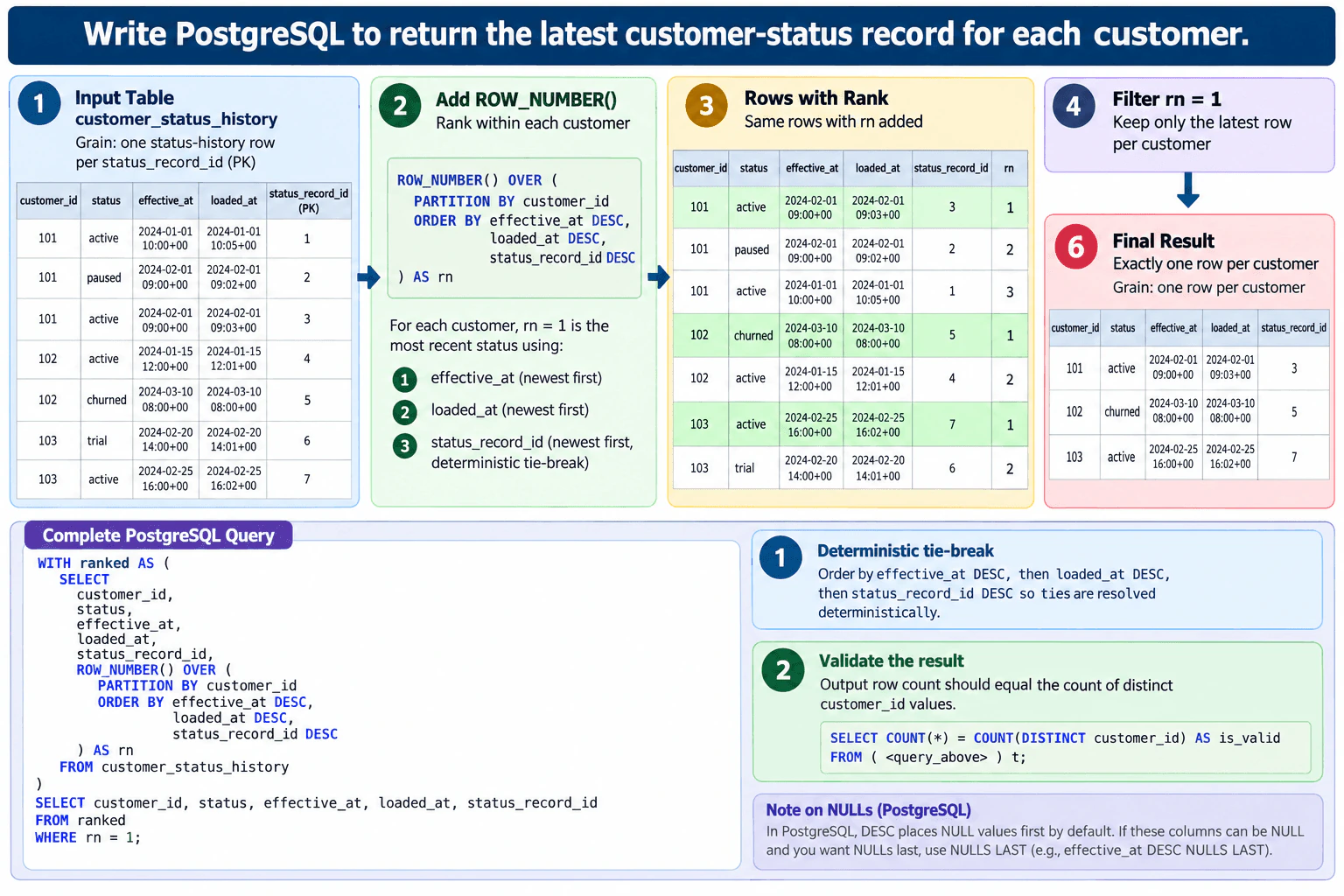
51. Write PostgreSQL to return the latest customer-status record for each customer.Sql And DatabasesMedium
i Question Details
Use customer_status_history(customer_id, status, effective_at timestamptz, loaded_at timestamptz, status_record_id primary key). Return exactly one row per customer using ROW_NUMBER. Rank by effective_at descending, then loaded_at descending, then status_record_id descending so ties are deterministic.
Short Interview Answer (30-60 seconds)
I would use ROW_NUMBER() because the requirement is exactly one row per customer. I partition by customer_id so each customer's history is ranked separately. Then I order by effective_at descending, loaded_at descending, and status_record_id descending. The newest effective record gets rn = 1; loaded_at resolves equal effective times, and the primary key is the final deterministic tie-breaker. I put that ranking in a CTE and filter to rn = 1.
Detailed Explanation
The table contains status history, so one customer may have several rows. The task is to return only the single row that represents each customer's latest status. I keep the input grain as one status-history record per row, then use ROW_NUMBER() to rank records separately inside each customer. The ranking checks effective_at first, loaded_at second, and status_record_id last. Finally, I keep only rn = 1. That changes the result grain to exactly one latest status record per customer while making ties deterministic.
Useful Questions to Ask the Interviewer
Can effective_at or loaded_at be NULL, and if so, should NULL timestamps be treated as older than known timestamps?
Does effective_at represent when the status became valid, while loaded_at represents when the record arrived in the database?
Should the output contain only the five supplied columns, or are additional history-table columns required?
How to Explain It in an Interview
The input table is customer_status_history(customer_id, status, effective_at, loaded_at, status_record_id). Its grain is one historical status record per row. There is no join in this problem, so there is no join-related row multiplication to manage.
A window function calculates a value across related rows without collapsing the rows. ROW_NUMBER() gives each row a unique sequential number inside its partition.
The partition is: PARTITION BY customer_id
This restarts numbering for each customer.
The required ordering is: ORDER BY effective_at DESC, loaded_at DESC, status_record_id DESC
The ordering has three levels. effective_at DESC puts the most recently effective record first. If two rows have the same effective_at, loaded_at DESC prefers the record loaded later. If both timestamps are equal, status_record_id DESC is the final tie-breaker. Because status_record_id is the primary key, it is unique, so the full ordering produces one deterministic winner.
The CTE named ranked keeps every source row and adds rn. The outer query then filters with WHERE rn = 1. The output grain is therefore one row per customer.
The PostgreSQL query is:
WITH ranked AS ( SELECT customer_id, status, effective_at, loaded_at, status_record_id, ROW_NUMBER() OVER ( PARTITION BY customer_id ORDER BY effective_at DESC, loaded_at DESC, status_record_id DESC ) AS rn FROM customer_status_history ) SELECT customer_id, status, effective_at, loaded_at, status_record_id FROM ranked WHERE rn = 1;
A concrete validation is to confirm that the output row count equals the number of distinct customer_id values in the source. I would also check that no customer_id appears more than once in the output.
NULL handling is an important edge case. In PostgreSQL, DESC places NULL values first by default. If effective_at or loaded_at can be NULL and NULL means unknown or older, I would explicitly use DESC NULLS LAST for those timestamp columns after confirming that business rule. I would not silently change the required ordering without that confirmation.
Because effective_at and loaded_at are timestamptz values, PostgreSQL compares their represented instants correctly even when display time zones differ. This query does not truncate dates or apply date boundaries, so no date function is needed.
ROW_NUMBER() is appropriate because the requirement is exactly one row per customer. RANK() is not the best fit because tied rows can share the same rank. The unique primary-key tie-breaker makes the ROW_NUMBER() result deterministic.
Technical Approach
1. Start from customer_status_history at one status-history record per row. 2. Partition records by customer_id. 3. Apply ROW_NUMBER() within each customer. 4. Order by effective_at DESC, then loaded_at DESC, then status_record_id DESC. 5. Store the ranking in a CTE. 6. Filter to rn = 1. 7. Validate that the output row count equals COUNT(DISTINCT customer_id) and that no customer appears more than once.
Practical Complexity & Trade-offs
The database must order records within each customer to assign ROW_NUMBER(). Without an already useful ordering path, processing the rows can require sorting, which is commonly about O(n log n) for n history rows. The actual PostgreSQL plan depends on the data and available indexes. Correctness comes from the complete three-column ordering; indexing is a separate performance decision that should be based on the real workload and execution plan.
Where it is used
This pattern is common when analysts need the current record from an append-only or historical table, such as the latest customer status, current account state, newest subscription state, latest workflow stage, or most recent value in a change-history table.
Why Interviewers Ask This
The interviewer is checking whether you understand data grain, PostgreSQL window functions, deterministic ordering, timestamp semantics, tie-breaking, and how to validate that a latest-record query returns exactly one row per customer.
Common interview mistakes
Common mistakes are using MAX(effective_at) alone and losing the rest of the selected row, assuming effective_at is always unique, omitting loaded_at or status_record_id from the tie-break order, using RANK() and potentially keeping multiple tied rows, filtering records before ranking when that changes what counts as latest, ignoring PostgreSQL's NULL ordering for DESC, or failing to verify that the result contains exactly one row per customer.
Interview tip
State the input and output grain first, then explain the three-level ordering before writing the SQL. Emphasize that status_record_id is the final deterministic tie-breaker, and finish with the validation check that output rows should equal distinct customers.
Interviewer may ask next
What would you change if effective_at or loaded_at can be NULL and NULL means the timestamp is unknown rather than newest?
I would make the NULL behavior explicit by using NULLS LAST for the nullable timestamp columns, for example ORDER BY effective_at DESC NULLS LAST, loaded_at DESC NULLS LAST, status_record_id DESC. I would first confirm that this matches the business meaning of NULL because PostgreSQL's default for DESC places NULL values first.
What would you do if this latest-per-customer query became slow on a very large history table?
I would keep the deterministic ranking logic unchanged and inspect the PostgreSQL execution plan. If this lookup is frequent, I would evaluate an index beginning with customer_id followed by the ordering columns, such as customer_id, effective_at DESC, loaded_at DESC, status_record_id DESC. Whether that index is worthwhile depends on table size, write volume, existing indexes, selectivity, and the observed plan, so performance tuning should not replace the correctness rules.
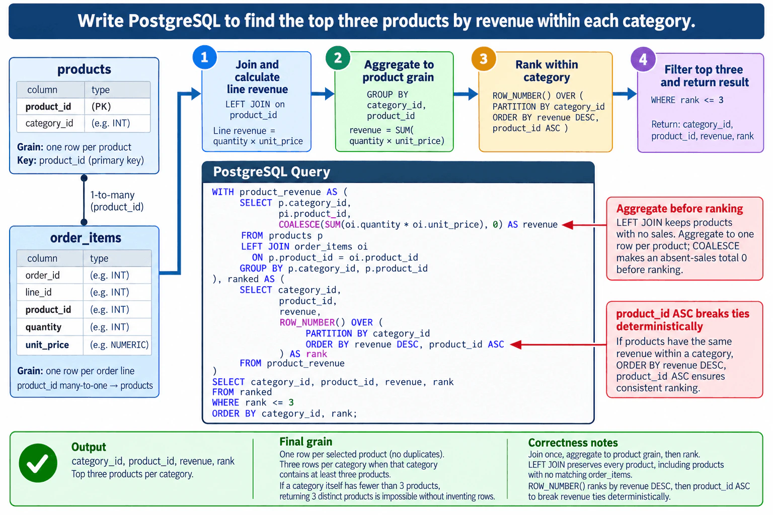
52. Write PostgreSQL to find the top three products by revenue within each category.Sql And DatabasesMedium
i Question Details
Use products(product_id primary key, category_id) and order_items(order_id, line_id, product_id, quantity, unit_price). Aggregate revenue to product grain before ranking. Return category_id, product_id, revenue, and rank; return exactly three products per category and break revenue ties by product_id ascending.
Short Interview Answer (30-60 seconds)
I would start from products, LEFT JOIN order_items on product_id, and aggregate quantity times unit_price to one row per product. COALESCE converts a missing sales total to zero so products without order rows can still be ranked. Then I would use ROW_NUMBER() partitioned by category_id and ordered by revenue descending, with product_id ascending as the deterministic tie-breaker. Finally, I would keep ranks 1 through 3. A category can return three distinct products only when it contains at least three products.
The key is to rank only after revenue is reduced to one row per product. The products table has one row per product, while order_items can contain many order lines for the same product. I start from products, LEFT JOIN the matching order lines, calculate line revenue as quantity times unit_price, and sum it by category and product. COALESCE gives a zero total to a product with no matching sales. Then ROW_NUMBER() ranks products separately inside each category, using product_id ascending to break equal-revenue ties consistently.
Useful Questions to Ask the Interviewer
Should products with no matching order_items remain eligible with zero revenue? The approved design does, so the query uses LEFT JOIN and COALESCE.
Can quantity or unit_price be NULL, and what business rule should apply to those incomplete order lines?
Should a category with fewer than three products simply return all products it has? Three distinct real products cannot be returned if fewer than three exist.
Is the supplied product_id relationship enforced so each order item maps to at most one product row? products.product_id is given as the primary key, which prevents multiple product matches for the same product_id.
How to Explain It in an Interview
First, define the grain. products is at product grain: one row per product because product_id is the primary key. order_items is at order-line grain, so the same product can appear on multiple rows. A join therefore creates one joined row for each matching order line. That row multiplication is expected, but ranking at that stage would be wrong because one product could appear several times.
The first CTE, product_revenue, changes the data back to product grain. It begins with products and LEFT JOINs order_items on product_id. Keeping products on the left preserves a product even when it has no matching order lines. Revenue is calculated as quantity * unit_price and summed for each category_id and product_id. COALESCE(SUM(...), 0) converts the absent-sales aggregate to zero. GROUP BY p.category_id, p.product_id therefore produces one ranking row per product.
The second CTE applies ROW_NUMBER(). A window function calculates a value across related rows while keeping each product row. PARTITION BY category_id creates a separate ranking for every category. ORDER BY revenue DESC puts the highest-revenue product first. product_id ASC is the secondary ordering rule, so equal-revenue products receive positions in a deterministic product_id order.
ROW_NUMBER() is the right choice for the stated requirement because it gives each product one unique position: 1, 2, 3, and so on. Using RANK() instead could assign the same rank to multiple tied products and could make a rank-based top-three filter return a different number of products. The required product_id tie-breaker also means equal revenue does not remain a ranking peer tie in this solution.
The outer query filters WHERE rank <= 3 and returns category_id, product_id, revenue, and rank. ORDER BY category_id, rank makes the displayed result easy to read. For every category that contains at least three products, the query returns exactly three product rows. If a category itself contains fewer than three products, returning three distinct real products is impossible without inventing rows.
For validation, I would confirm that product_revenue contains one row per product_id and no duplicate product rows. I would compare the aggregated revenue with an independently calculated order-line revenue control total, using the same NULL policy. I would test two products with equal revenue to confirm the lower product_id gets the earlier rank, test a product with no order_items to confirm zero revenue, and verify that every category with at least three products has ranks 1, 2, and 3. No date-boundary logic is needed because the supplied schema and question contain no date field or reporting window.
Technical Approach
1. Start from products so every product remains in the ranking population. 2. LEFT JOIN order_items on product_id. 3. Calculate line revenue as quantity * unit_price. 4. GROUP BY category_id and product_id and SUM line revenue to reach one row per product. 5. Use COALESCE on the aggregate so a product with no matching order_items has revenue 0. 6. Apply ROW_NUMBER() OVER (PARTITION BY category_id ORDER BY revenue DESC, product_id ASC). 7. Filter to rank <= 3. 8. Return category_id, product_id, revenue, and rank, ordered by category_id and rank. 9. Validate product grain, revenue totals, zero-sales behavior, tie-breaking, and per-category row counts.
Practical Complexity & Trade-offs
The query must read the relevant product and order-item rows, join them, aggregate the order lines to product grain, and then sort products within categories for ROW_NUMBER(). If N is the number of order-item rows and P is the number of products, the aggregation work grows roughly with the rows processed, while ranking requires sorting the P product-level rows, commonly about O(P log P) for the sorting work. Real PostgreSQL performance depends on data size, statistics, indexes, memory, and the execution plan, so correctness should be verified before performance tuning.
Example
The implementation uses two CTEs. product_revenue preserves all products with a LEFT JOIN and aggregates revenue to one row per product. ranked then uses ROW_NUMBER() to assign a unique position within each category, ordered by revenue descending and product_id ascending. The outer query keeps positions 1 through 3.
Code
WITH
product_revenue AS (
SELECT
p.category_id,
p.product_id,
COALESCE(SUM(oi.quantity * oi.unit_price), 0) AS revenue
FROM
products p
LEFTJOIN order_items oi ON p.product_id = oi.product_id
GROUPBY
p.category_id,
p.product_id
),
ranked AS (
SELECT
category_id,
product_id,
revenue,
ROW_NUMBER() OVER (
PARTITIONBY
category_id
ORDERBY
revenue DESC,
product_id ASC
) AS rank
FROM
product_revenue
)
SELECT
category_id,
product_id,
revenue,
rank
FROM
ranked
WHERE
rank <=3ORDERBY
category_id,
rank;
Where it is used
This pattern is common in sales reporting, category dashboards, merchandising analysis, marketplace analytics, and other top-N-per-group reports where transaction-level rows must first be aggregated to an entity such as a product before ranking.
Why Interviewers Ask This
This tests whether the candidate understands data grain, one-to-many joins, aggregation before ranking, window functions, deterministic tie-breaking, NULL handling, and validation. The key judgment is recognizing that order_items is lower-grain data than the requested product-level result, so revenue must be aggregated to one row per product before products are ranked inside each category.
Common interview mistakes
Ranking order_items before aggregating to product grain; using RANK() when the requirement calls for a unique deterministic top-three selection; omitting product_id ASC and leaving equal-revenue ordering nondeterministic; using an INNER JOIN when products without sales must remain eligible; forgetting COALESCE for a product with no matching order rows; grouping at the wrong grain; assuming rank <= 3 can manufacture three products when a category contains fewer than three products; and failing to validate totals after the one-to-many join.
Interview tip
Explain the grain before the SQL: order_items is order-line grain, but ranking must happen at product grain. Then describe the query as join, aggregate, rank, and filter. Explicitly mention why ROW_NUMBER() and product_id ASC make the top three deterministic, and call out the fewer-than-three-products boundary.
Interviewer may ask next
What changes if quantity or unit_price can be NULL?
In PostgreSQL, quantity * unit_price becomes NULL when either value is NULL, and SUM ignores NULL inputs. I would not automatically replace those source values with zero unless that matches the business rule. I would first clarify whether incomplete order lines should be excluded, rejected as data-quality errors, or treated as zero. After applying that agreed rule, I would validate the product totals against an independent revenue control total using the same NULL treatment.
What would you change if the business wanted every product tied at the third-highest revenue instead of exactly three products?
I would change the ranking semantics. The current ROW_NUMBER() intentionally assigns unique positions and returns at most three products. If every product tied at the third revenue level must be included, I would rank by revenue alone with DENSE_RANK() or RANK(), depending on the desired gap behavior, and filter that revenue rank to <= 3. I would not put product_id inside that ranking ORDER BY because it would split equal-revenue products into different peer groups; product_id could instead be used only in the final display ORDER BY for deterministic presentation.
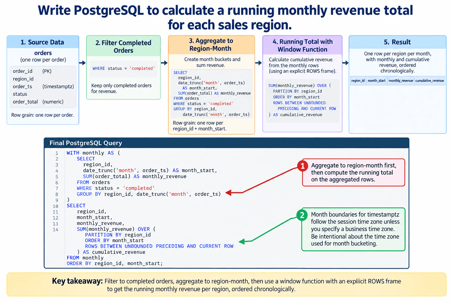
53. Write PostgreSQL to calculate a running monthly revenue total for each sales region.Sql And DatabasesMedium
i Question Details
Use orders(order_id primary key, region_id, order_ts timestamptz, status, order_total numeric). Aggregate completed revenue to region-month grain first. Return region_id, month_start, monthly_revenue, and cumulative_revenue using an explicit ROWS window frame, ordered chronologically within each region.
Short Interview Answer (30-60 seconds)
I would first filter to completed orders and aggregate revenue to one row per region and month. Then I would apply a windowed SUM over those monthly rows, partitioned by region and ordered by month. I would use an explicit ROWS BETWEEN UNBOUNDED PRECEDING AND CURRENT ROW frame so the cumulative total clearly means all monthly rows from the first month through the current month. Because order_ts is timestamptz, I would also confirm which time zone defines the business month boundaries.
The safest approach is to solve this in two stages. First, keep only completed orders and reduce the order-level data to one row per sales region and month. That produces monthly_revenue at the correct reporting grain. Second, calculate cumulative_revenue from those monthly rows with a window function. The window restarts for each region and moves chronologically by month. An explicit ROWS frame makes the running-total boundary clear. Because order_ts is timestamptz, the month boundary also depends on the intended time zone, so that setting should be confirmed before production use.
Useful Questions to Ask the Interviewer
Which business time zone should define the start and end of a month?
Should a NULL order_total be ignored, treated as zero, or rejected as bad data?
Should months with no completed orders appear as zero-revenue rows, or can they be absent?
How to Explain It in an Interview
The input grain is one row per order because order_id is the primary key. The required output grain is one row per region and month. There are no joins in this problem, so there is no join-driven row multiplication to manage.
Start by filtering with status = 'completed'. In SQL three-valued logic, a row whose status is NULL does not satisfy that equality predicate, so it is excluded.
Next, use date_trunc('month', order_ts) to derive month_start and GROUP BY region_id plus that month expression. SUM(order_total) then produces monthly_revenue at exactly the required region-month grain. This aggregation must happen before the running calculation. If the window were applied directly to the order rows, the result would be an order-level cumulative total instead of the requested monthly cumulative total.
Then use SUM(monthly_revenue) OVER (...). PARTITION BY region_id creates a separate running sequence for each region. ORDER BY month_start processes the monthly rows chronologically. ROWS BETWEEN UNBOUNDED PRECEDING AND CURRENT ROW explicitly says to include every monthly row from the first row in that region's partition through the current row.
The final ORDER BY region_id, month_start controls the displayed result order so each region's rows appear chronologically.
There are several important data checks. Because order_ts is timestamptz, date_trunc('month', order_ts) uses the applicable session time-zone interpretation for month boundaries unless the query explicitly converts to an agreed business time zone first. SUM ignores NULL order_total values. If every qualifying order_total in a region-month group is NULL, monthly_revenue is NULL. I would only use COALESCE if the business rule explicitly says that a missing amount should mean zero.
This query also does not create missing calendar months. If a region has no completed orders in a month, there is no row for that region-month. If zero-revenue months must be shown, I would build a complete region-month calendar, LEFT JOIN the monthly aggregate to it, convert the missing monthly revenue to zero according to that business rule, and then calculate the running total.
For validation, I would compare the sum of monthly_revenue with an independent SUM(order_total) over the same completed-order population and the same month-boundary definition. I would also verify that the monthly CTE has exactly one row for each returned region_id and month_start combination. Finally, for each region, the final non-NULL cumulative_revenue should reconcile with the cumulative sum of that region's monthly revenue values under the same NULL-handling rules.
Technical Approach
Read orders at one-row-per-order grain.
Filter to status = 'completed'.
Derive month_start with date_trunc('month', order_ts), using the intended business time-zone convention.
GROUP BY region_id and month_start and calculate SUM(order_total) AS monthly_revenue.
Apply SUM(monthly_revenue) OVER (PARTITION BY region_id ORDER BY month_start ROWS BETWEEN UNBOUNDED PRECEDING AND CURRENT ROW).
Return region_id, month_start, monthly_revenue, and cumulative_revenue.
Order the final output by region_id and month_start.
Validate the region-month totals and final cumulative totals against the completed-order source population.
Practical Complexity & Trade-offs
The database must read the qualifying orders, group them into region-month rows, and order those monthly rows within each region for the window calculation. The exact runtime depends on data size, indexes, memory, and PostgreSQL's execution plan. Conceptually, grouping and sorting are the main costs. The window calculation itself operates on the much smaller region-month result rather than directly on every order row.
Example
Use a CTE to make the grain change explicit. The CTE filters completed orders and produces exactly one row per returned region and month with monthly_revenue. The outer query then applies the running SUM to those aggregated monthly rows. This keeps the aggregation stage separate from the window-function stage and matches the approved diagram.
Code
WITH
monthly AS (
SELECT
region_id,
date_trunc ('month', order_ts) AS month_start,
SUM(order_total) AS monthly_revenue
FROM
orders
WHERE
status ='completed'GROUPBY
region_id,
date_trunc ('month', order_ts)
)
SELECT
region_id,
month_start,
monthly_revenue,
SUM(monthly_revenue) OVER (
PARTITIONBY
region_id
ORDERBY
month_start ROWSBETWEEN UNBOUNDED PRECEDING
ANDCURRENTROW
) AS cumulative_revenue
FROM
monthly
ORDERBY
region_id,
month_start;
Where it is used
This pattern is common in finance and analytics reporting for cumulative revenue, cumulative sales, running costs, and other metrics that must first be summarized to a reporting period before a running total is calculated.
Why Interviewers Ask This
The interviewer is checking whether you understand data grain, filtering, PostgreSQL date handling, aggregation, and window functions well enough to calculate a running monthly metric without applying the cumulative sum at the wrong grain.
Common interview mistakes
Common mistakes are calculating the running SUM directly on order-level rows instead of aggregating to region-month first; forgetting PARTITION BY region_id and mixing regions together; omitting ORDER BY month_start; relying on an implicit window frame instead of the requested explicit ROWS frame; assuming timestamptz month boundaries are independent of time zone; assuming missing months automatically appear; and using COALESCE on NULL revenue without confirming that NULL should mean zero.
Interview tip
State the grain change before writing the SQL: 'The source is one row per order, but the running total must operate on one row per region-month.' Then write the monthly CTE first and the window calculation second. Mention the timestamptz month-boundary question as an important production data check.
Interviewer may ask next
What changes if months with no completed orders must still appear with zero monthly revenue?
The current query returns only region-month combinations that have at least one completed order. To include missing months, create or use a calendar of month_start values, combine it with the required regions, LEFT JOIN the aggregated monthly revenue, and use COALESCE(monthly_revenue, 0) only because the requirement explicitly defines a missing month as zero revenue. Then calculate the same running SUM over that complete region-month series.
What if the business defines months in a specific time zone instead of the PostgreSQL session time zone?
Convert order_ts to the agreed business time-zone interpretation before deriving month_start, and use that same convention everywhere the month boundary matters. This prevents orders near UTC offsets or daylight-saving transitions from being assigned to a different business month than intended. The filtering, aggregation, validation, and reporting logic should all use the same explicit time-zone definition.
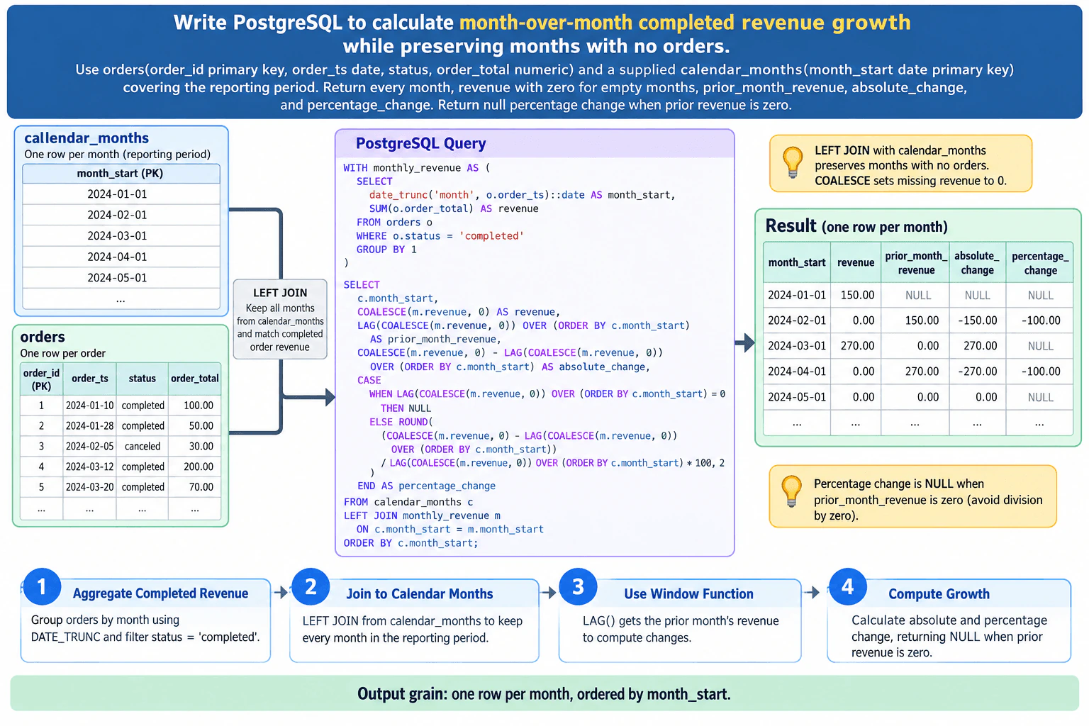
54. Write PostgreSQL to calculate month-over-month completed revenue growth while preserving months with no orders.Sql And DatabasesMedium
i Question Details
Use orders(order_id primary key, order_ts date, status, order_total numeric) and a supplied calendar_months(month_start date primary key) covering the reporting period. Return every month, revenue with zero for empty months, prior_month_revenue, absolute_change, and percentage_change. Return null percentage change when prior revenue is zero.
Short Interview Answer (30-60 seconds)
I would first aggregate completed orders to one row per month. Then I would start from calendar_months and LEFT JOIN that monthly revenue so every reporting month survives, using COALESCE to turn missing revenue into zero. After the join is at one-row-per-month grain, I would use LAG ordered by month_start to get prior_month_revenue. Absolute change is current revenue minus prior revenue. Percentage change is that difference divided by prior revenue, but I return NULL when the prior revenue is zero. Finally, I order by month_start.
The goal is to return one row for every supplied reporting month, even when that month has no completed orders. The orders table starts at one row per order, so I first filter to completed orders and aggregate order_total to month level. Then I use calendar_months as the left side of a LEFT JOIN. This keeps every calendar month and lets COALESCE turn missing monthly revenue into zero. Once the data is one row per month, LAG can safely read the previous month's revenue. Growth percentage is NULL when the previous revenue is zero.
Useful Questions to Ask the Interviewer
Should only rows with status = 'completed' contribute to revenue, with all other statuses excluded?
Does calendar_months already contain exactly the reporting months that should appear in the output?
Can order_total be NULL, and if so, should NULL amounts be ignored by SUM or treated as zero?
Should percentage_change be returned as a percentage value such as 25.00 for 25%?
Is order_ts already expressed in the reporting calendar, with no time-zone conversion needed?
How to Explain It in an Interview
The important part is the grain. orders has one row per order, while the final result must have one row per calendar month. If I join raw orders directly to calendar_months and then calculate LAG, a month could have many order rows and the previous-row value would not mean previous-month revenue. So I aggregate first.
The first CTE filters orders to status = 'completed', converts order_ts to the first day of its month with date_trunc('month', order_ts)::date, and SUMs order_total. That produces at most one revenue row for each month that has completed orders.
Next, I start from calendar_months and LEFT JOIN the monthly aggregation on month_start. calendar_months is the preserved side because the requirement is to return every supplied month. A month with no matching completed orders receives NULL from the joined revenue column, so COALESCE(m.revenue, 0) converts that missing value to zero.
After that join, the row grain is exactly one row per supplied month because calendar_months.month_start is a primary key and the monthly aggregation has one row per month. This prevents row multiplication and makes the window calculation reliable.
LAG(COALESCE(m.revenue, 0)) OVER (ORDER BY c.month_start) returns the revenue from the immediately preceding supplied calendar row. The first month has no preceding row, so prior_month_revenue is NULL. The absolute change is current revenue minus that prior value, so it is also NULL for the first month.
For percentage change, dividing by zero is not meaningful. I use a CASE expression: when prior_month_revenue is zero, return NULL; otherwise calculate ((current revenue - prior revenue) / prior revenue) * 100. If there is no prior month, LAG returns NULL and the arithmetic also returns NULL.
A useful validation is to confirm that the final row count equals the number of rows in calendar_months for the reporting period. I would also compare the sum of returned monthly revenue with an independent SUM(order_total) over completed orders restricted to the same reporting period. Finally, I would test the first month, an empty month, a month following zero revenue, and consecutive zero-revenue months.
Technical Approach
1. Treat calendar_months as the required output population: one row per reporting month. 2. Filter orders to status = 'completed'. 3. Convert each completed order date to its month start with date_trunc('month', order_ts)::date. 4. GROUP BY that month and SUM(order_total), producing at most one revenue row per month. 5. LEFT JOIN the monthly aggregation to calendar_months so months without orders remain present. 6. Use COALESCE on joined revenue so an empty month has revenue = 0. 7. Use LAG over ORDER BY month_start to obtain prior_month_revenue. 8. Calculate absolute_change as revenue - prior_month_revenue. 9. Calculate percentage_change as 100 * absolute_change / prior_month_revenue, returning NULL when prior revenue is zero. 10. ORDER BY month_start and validate row counts and revenue totals.
Practical Complexity & Trade-offs
The query reads the completed-order rows, groups them by month, joins that monthly result to the supplied calendar, and then processes the monthly rows in month_start order for LAG. The main cost is usually scanning and grouping orders. The window calculation operates only after the data has been reduced to monthly grain. An index may help in a real workload, but the best index depends on table size, data distribution, filters, and the execution plan; no particular index is required for correctness.
Example
Aggregate completed orders to monthly grain first, then LEFT JOIN that result to the supplied calendar. COALESCE converts missing monthly revenue to zero. Apply LAG only after the join has produced one row per month, so the previous row represents the previous supplied calendar month. The query repeats the LAG expression to stay consistent with the approved diagram; an additional CTE could calculate prior_month_revenue once if maintainability were more important than matching that presentation exactly.
Code
WITH
monthly_revenue AS (
SELECTCAST(date_trunc ('month', o.order_ts) ASdate) AS month_start,
SUM(o.order_total) AS revenue
FROM
orders AS o
WHERE
o.status ='completed'GROUPBY1
)
SELECT
c.month_start,
COALESCE(m.revenue, 0) AS revenue,
LAG (COALESCE(m.revenue, 0)) OVER (
ORDERBY
c.month_start
) AS prior_month_revenue,
COALESCE(m.revenue, 0) -LAG (COALESCE(m.revenue, 0)) OVER (
ORDERBY
c.month_start
) AS absolute_change,
CASEWHENLAG (COALESCE(m.revenue, 0)) OVER (
ORDERBY
c.month_start
) =0THENNULLELSE ROUND(
(
COALESCE(m.revenue, 0) -LAG (COALESCE(m.revenue, 0)) OVER (
ORDERBY
c.month_start
)
) /LAG (COALESCE(m.revenue, 0)) OVER (
ORDERBY
c.month_start
) *100,
2
)
ENDAS percentage_change
FROM
calendar_months AS c
LEFTJOIN monthly_revenue AS m ON c.month_start = m.month_start
ORDERBY
c.month_start;
Where it is used
This pattern is common in monthly revenue reporting, finance dashboards, subscription reporting, sales trend analysis, and other time-series reports where periods with no activity must still appear instead of disappearing from the result.
Why Interviewers Ask This
The interviewer is testing whether you can control SQL grain, preserve missing time periods, aggregate only the required population, use a window function at the correct grain, and handle zero or missing prior-month values without producing incorrect growth percentages.
Common interview mistakes
Common mistakes are starting from orders instead of calendar_months, which drops empty months; joining raw order rows before reducing them to monthly grain, which can create multiple rows per month; using an INNER JOIN, which removes months without orders; applying LAG before missing months have been restored; leaving empty-month revenue as NULL instead of zero; dividing by prior revenue without handling zero; forgetting that the first month has no prior value; and omitting ORDER BY month_start from the window definition.
Interview tip
State the grain before writing SQL: orders is one row per order, monthly_revenue is one row per month with completed orders, and the final result is one row per supplied calendar month. Then explain why calendar_months must drive the LEFT JOIN and why LAG belongs after the data has reached monthly grain.
Interviewer may ask next
What happens when a month has zero revenue and the following month has positive revenue?
The zero-revenue month is preserved because calendar_months drives the LEFT JOIN and its revenue is COALESCEd to 0. In the following month, prior_month_revenue is therefore 0. absolute_change is current revenue minus 0, but percentage_change is NULL because a percentage growth calculation cannot use zero as the prior-revenue denominator.
How would you change the query if calendar_months could contain gaps and the business required comparison with the immediately previous chronological month, even when that month was missing from the supplied calendar?
LAG compares adjacent rows in the supplied result, so the current query assumes calendar_months contains each reporting month in sequence. If that assumption changes, I would first use a complete monthly calendar covering the required date range, join revenue to that complete series, and then apply LAG. That prevents two non-adjacent calendar months from being treated as consecutive months.
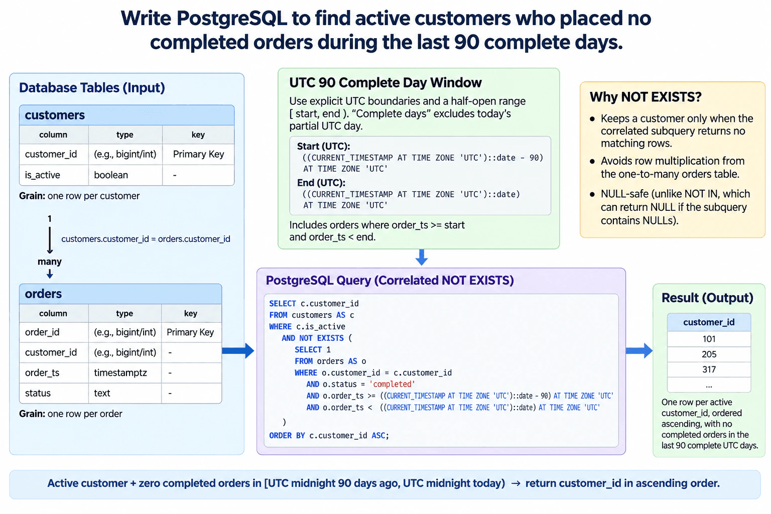
55. Write PostgreSQL to find active customers who placed no completed orders during the last 90 complete days.Sql And DatabasesMedium
i Question Details
Use customers(customer_id primary key, is_active boolean) and orders(order_id primary key, customer_id, order_ts timestamptz, status). Use an anti-join or NOT EXISTS, define the UTC date boundary explicitly, avoid null-sensitive NOT IN behavior, and return customer_id ordered ascending.
Short Interview Answer (30-60 seconds)
I would start from active customers and use a correlated NOT EXISTS against orders. The subquery looks only for status = 'completed' and order timestamps from UTC midnight 90 days ago, inclusive, up to UTC midnight today, exclusive. If no such order exists, the customer is returned. NOT EXISTS avoids row multiplication and avoids the NULL-sensitive behavior of NOT IN. Then I sort customer_id ascending.
The task is to return active customers who had zero completed orders during the last 90 full UTC days. The customers table has one row per customer, while orders has one row per order, so one customer can have many orders. The output must stay at one row per customer. A correlated NOT EXISTS is a good fit because it tests for qualifying orders without multiplying customer rows. The time window starts at UTC midnight 90 days ago and ends at UTC midnight today, so today's incomplete UTC day is excluded. The final output is customer_id in ascending order.
Useful Questions to Ask the Interviewer
Should the order status match the exact value 'completed', including case?
Is "last 90 complete days" defined exactly as the 90 full UTC calendar days before today?
Can orders.customer_id be NULL or contain values that do not match a current customer?
Should an active customer with no orders at all be included? Under this requirement, yes.
How to Explain It in an Interview
First, define the grain. customers has one row per customer because customer_id is its primary key. orders has one row per order because order_id is its primary key. The relationship is one customer to many orders through customers.customer_id = orders.customer_id.
The required result must remain at one row per customer. A normal one-to-many join can create several rows for the same customer when multiple orders match. A correlated NOT EXISTS avoids that row multiplication. For each active customer, the subquery asks whether any completed order exists inside the required UTC window. NOT EXISTS keeps the customer only when the subquery finds no qualifying row.
The date range is a half-open interval: [start, end). The start is UTC midnight 90 days ago and is inclusive. The end is UTC midnight today and is exclusive. Therefore an order exactly at the start boundary is inside the window, while an order exactly at today's UTC midnight is outside it. This represents exactly the 90 complete UTC calendar days before today and excludes today's partial day.
The boundary expressions explicitly use UTC. (CURRENT_TIMESTAMP AT TIME ZONE 'UTC')::date derives today's UTC calendar date. Subtracting 90 gives the start date. Applying AT TIME ZONE 'UTC' to those midnight timestamp values produces timestamptz boundaries suitable for comparison with orders.order_ts, which is also timestamptz.
Inside the correlated subquery, three conditions define a disqualifying order: the order belongs to the current customer, its status is exactly 'completed', and its order_ts is greater than or equal to the start boundary and less than the end boundary. If at least one row satisfies all three, EXISTS is true, so NOT EXISTS is false and that customer is excluded.
NOT EXISTS is preferable here to customer_id NOT IN (subquery) because NOT IN follows SQL three-valued logic. If a NOT IN subquery produces a NULL value, the comparison can become unknown and lead to unexpected filtering. The correlated NOT EXISTS test does not have that NULL-sensitive membership behavior.
There is no need for GROUP BY, HAVING, DISTINCT, or a window function. NOT EXISTS keeps the customer-level grain even when a customer has many orders. ORDER BY c.customer_id ASC then returns the qualifying customer IDs in the required ascending order.
For validation, test an active customer with no orders, one with only non-completed orders, one with a completed order just before the start boundary, one exactly at the start boundary, one just before today's UTC midnight, and one exactly at today's UTC midnight. Also verify that every returned customer is active, no returned customer has a completed order in the target window, and the final customer_id values contain no duplicates.
Technical Approach
Start from customers at one row per customer.
Filter to active customers.
Define the start boundary as UTC midnight 90 days ago and the end boundary as UTC midnight today.
Use a correlated NOT EXISTS against orders for the same customer_id.
In the subquery, require status = 'completed', order_ts >= start, and order_ts < end.
Keep only customers for whom no qualifying order exists.
Return customer_id ordered ascending.
Validate activity status, uniqueness, NULL behavior, and both UTC boundaries.
Practical Complexity & Trade-offs
The query logically compares active customers with qualifying orders. The real execution cost depends on table sizes, data distribution, statistics, and available indexes. NOT EXISTS avoids creating duplicate customer rows, which keeps the result grain simple. On large tables, an index that supports the customer, status, and timestamp predicates may improve performance, but the best index should be confirmed with the actual workload and PostgreSQL execution plan rather than assumed from the question alone.
Example
PostgreSQL implementation using a correlated NOT EXISTS anti-join and explicit UTC midnight boundaries. The half-open interval includes UTC midnight 90 days ago and excludes UTC midnight today.
Code
SELECT
c.customer_id
FROM
customers AS c
WHERE
c.is_active
ANDNOTEXISTS (
SELECT1FROM
orders AS o
WHERE
o.customer_id = c.customer_id
AND o.status ='completed'AND o.order_ts >= (
CAST(CURRENT_TIMESTAMPATTIME ZONE 'UTC'ASdate) -90
) ATTIME ZONE 'UTC'AND o.order_ts <CAST(CURRENT_TIMESTAMPATTIME ZONE 'UTC'ASdate) ATTIME ZONE 'UTC'
)
ORDERBY
c.customer_id ASC;
Where it is used
This anti-join pattern is useful for finding customers with no recent completed purchases, subscribers with no successful payments, users with no qualifying activity in a reporting window, or any situation where a parent row should be returned only when no matching child row exists.
Why Interviewers Ask This
This tests whether the candidate can reason correctly about one-to-many relational data, anti-joins, UTC date boundaries, NULL behavior, row grain, and deterministic ordering, rather than only writing syntactically valid SQL.
Common interview mistakes
Using NOT IN without considering NULLs; using a rolling 90-day timestamp interval instead of 90 complete UTC calendar days; including today's partial day; using an inclusive end boundary instead of a half-open range; joining orders directly and accidentally duplicating customers; forgetting the status = 'completed' filter; or omitting the required ascending ordering.
Interview tip
State the customer and order row grain first, then define the UTC half-open interval. After that, explain why NOT EXISTS preserves one row per customer and avoids the NULL-sensitive behavior of NOT IN.
Interviewer may ask next
What happens to an active customer who has no orders at all, or only non-completed orders?
The customer is returned. For that customer, the correlated subquery finds no row satisfying all required conditions: matching customer_id, status = 'completed', and order_ts inside the 90-complete-day UTC window. Therefore NOT EXISTS evaluates to true.
How would you change the query if the requirement became the last 90 rolling 24-hour periods instead of 90 complete UTC calendar days?
Replace the UTC calendar-midnight boundaries with an instant-based window from CURRENT_TIMESTAMP - INTERVAL '90 days' up to CURRENT_TIMESTAMP. That changes the meaning from 90 complete UTC dates to the immediately preceding 90 times 24 hours, so the current partial day is included.
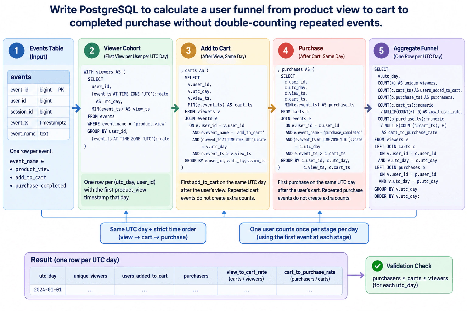
56. Write PostgreSQL to calculate a user funnel from product view to cart to completed purchase without double-counting repeated events.Sql And DatabasesMedium
i Question Details
Use events(user_id, session_id, event_id primary key, event_ts timestamptz, event_name) with event_name values product_view, add_to_cart, and purchase_completed. For each UTC day, return unique viewers, users who added to cart after viewing that day, purchasers after adding to cart that day, view_to_cart_rate, and cart_to_purchase_rate. Each user contributes at most once per stage per day.
Short Interview Answer (30-60 seconds)
I would build the funnel at one row per user per UTC day. First, I take each user's earliest product_view that day. Then I find that user's earliest add_to_cart on the same UTC day strictly after the view, and finally the earliest purchase_completed strictly after that cart. Because each CTE has at most one row per user-day, repeated events cannot double-count the user. I LEFT JOIN the stages back to viewers, aggregate by UTC day, and calculate view-to-cart as carts divided by viewers and cart-to-purchase as purchasers divided by carts, using NULLIF to avoid division by zero.
The task is to build a daily funnel that counts people, not raw events. The source table has one row per event, so one user may view, add to cart, or purchase several times. For each UTC day, we first keep one qualifying product view per user. Then we keep one cart event that occurs later that same day, followed by one purchase that occurs later than the cart. This gives one row per user per stage per day. Finally, we group by UTC day and calculate counts and conversion rates without repeated events increasing the totals.
Useful Questions to Ask the Interviewer
Should a cart and purchase count only when they happen on the same UTC day as the user's qualifying view?
Does "after" mean strictly later timestamps, so events with identical timestamps should not qualify as the next stage?
Should the funnel be user-based across sessions, or must all three events occur in the same session_id?
Are user_id and event_ts guaranteed to be non-NULL for these funnel events, or should invalid rows be excluded explicitly?
How to Explain It in an Interview
The important idea is data grain. The input grain is one event row, identified by event_id as the primary key. The intermediate grain should become one row per (utc_day, user_id), so repeated events cannot multiply a user. The final output grain is one row per UTC day.
I would use three CTEs that match the diagram's flow: viewers, carts, and purchases.
Viewer cohort: For every user and UTC date, select MIN(event_ts) for product_view. (event_ts AT TIME ZONE 'UTC')::date creates the requested UTC calendar day from the timestamptz value. The result has one row per user-day and the first view timestamp for that day.
Add to cart: Join each viewer row to events for the same user. Restrict event_name to add_to_cart, require the event's UTC date to equal the viewer's utc_day, and require event_ts > view_ts. Taking MIN(event_ts) produces the first qualifying cart after the user's first view. Grouping at the viewer user-day grain prevents repeated cart events from creating extra users.
Purchase: Join each cart row to events for the same user and UTC day. Keep purchase_completed events with event_ts > cart_ts, then take MIN(event_ts). That gives the first qualifying purchase after the cart while ignoring repeated purchases.
Aggregate funnel: Start from viewers because every reported funnel row is defined by a viewing cohort. LEFT JOIN carts and purchases on both user_id and utc_day. COUNT(*) gives unique viewers because viewers already has one row per user-day. COUNT(c.cart_ts) gives users who reached cart, and COUNT(p.purchase_ts) gives purchasers.
Rates: view_to_cart_rate = carts / viewers and cart_to_purchase_rate = purchasers / carts. Cast the numerator to numeric so PostgreSQL performs non-integer division. NULLIF(denominator, 0) prevents a division-by-zero error. With this design, a day that has viewers but no carts produces a NULL cart-to-purchase rate because there is no valid denominator.
The join grain matters. Joining raw view, cart, and purchase events directly could create row multiplication. For example, multiple views joined to multiple carts could create several rows for one user. Reducing each stage to one row per user-day before the final joins avoids that failure.
NULL behavior should also be explicit. The final LEFT JOIN intentionally produces NULL cart_ts or purchase_ts for users who stop before a later funnel stage, and COUNT(column) ignores those NULLs. The query assumes user_id and event_ts are usable identifiers and timestamps for funnel events. If either can be NULL in the source, I would treat those rows as data-quality failures or filter them according to the data contract before calculating the funnel.
The UTC boundary is part of correctness. The query derives utc_day from each event using AT TIME ZONE 'UTC' before casting to date. A cart or purchase on a different UTC date is not included in the original day's funnel, even if it is only a few minutes later in another local time zone.
The strict > comparisons also define ordering. A cart must occur strictly after the selected view, and a purchase must occur strictly after the selected cart. If the business wants equal timestamps to count, that rule would need to change explicitly.
A window function such as ROW_NUMBER could also be used to select the first event at each stage, but it is unnecessary here because MIN(event_ts) at the correct user-day grain expresses the requirement more directly.
A concrete validation is purchasers <= users_added_to_cart <= unique_viewers for every UTC day, matching the diagram. I would also compare the viewer count against an independent COUNT(DISTINCT user_id) over product_view events grouped by the same UTC date. For individual test users, I would inspect the selected view_ts, cart_ts, and purchase_ts to confirm strict ordering and same-day behavior.
A PostgreSQL implementation consistent with that plan is:
WITH viewers AS ( SELECT user_id, (event_ts AT TIME ZONE 'UTC')::date AS utc_day, MIN(event_ts) AS view_ts FROM events WHERE event_name = 'product_view' GROUP BY user_id, (event_ts AT TIME ZONE 'UTC')::date ), carts AS ( SELECT v.user_id, v.utc_day, v.view_ts, MIN(e.event_ts) AS cart_ts FROM viewers v JOIN events e ON e.user_id = v.user_id AND e.event_name = 'add_to_cart' AND (e.event_ts AT TIME ZONE 'UTC')::date = v.utc_day AND e.event_ts > v.view_ts GROUP BY v.user_id, v.utc_day, v.view_ts ), purchases AS ( SELECT c.user_id, c.utc_day, c.view_ts, c.cart_ts, MIN(e.event_ts) AS purchase_ts FROM carts c JOIN events e ON e.user_id = c.user_id AND e.event_name = 'purchase_completed' AND (e.event_ts AT TIME ZONE 'UTC')::date = c.utc_day AND e.event_ts > c.cart_ts GROUP BY c.user_id, c.utc_day, c.view_ts, c.cart_ts ) SELECT v.utc_day, COUNT(*) AS unique_viewers, COUNT(c.cart_ts) AS users_added_to_cart, COUNT(p.purchase_ts) AS purchasers, COUNT(c.cart_ts)::numeric / NULLIF(COUNT(*), 0) AS view_to_cart_rate, COUNT(p.purchase_ts)::numeric / NULLIF(COUNT(c.cart_ts), 0) AS cart_to_purchase_rate FROM viewers v LEFT JOIN carts c ON v.user_id = c.user_id AND v.utc_day = c.utc_day LEFT JOIN purchases p ON v.user_id = p.user_id AND v.utc_day = p.utc_day GROUP BY v.utc_day ORDER BY v.utc_day;
This favors correctness and clarity. On a large events table, repeatedly joining and filtering the same source can be expensive, so I would inspect the query plan and consider indexes only after confirming the actual workload and selectivity. The correctness rule should remain unchanged: one user per UTC day, same-day stage progression, and strict view -> cart -> purchase ordering.
Technical Approach
Define the input grain as one event row and the output grain as one row per UTC day.
Build a viewers CTE with the earliest product_view for each user and UTC day.
Join viewers to add_to_cart events for the same user and UTC day with event_ts > view_ts, then keep the earliest qualifying cart.
Join carts to purchase_completed events for the same user and UTC day with event_ts > cart_ts, then keep the earliest qualifying purchase.
LEFT JOIN carts and purchases back to viewers on user_id and utc_day so users who stop early remain in the funnel.
GROUP BY utc_day and count viewers, carts, and purchasers.
Calculate view_to_cart_rate as carts/viewers and cart_to_purchase_rate as purchasers/carts using numeric division and NULLIF.
Validate purchasers <= carts <= viewers and inspect edge cases around duplicates, equal timestamps, NULLs, and UTC date boundaries.
Practical Complexity & Trade-offs
The query must examine the relevant events and perform joins back to the events table for later funnel stages. Its real cost depends on table size, filtering selectivity, indexes, and PostgreSQL's chosen execution plan. The design intentionally reduces each funnel stage to one row per user-day before final aggregation, which prevents row multiplication and keeps the final joins simple. Correctness should be established first; performance tuning should follow from EXPLAIN or EXPLAIN ANALYZE on the real workload rather than assuming a specific index strategy.
Example
Use staged PostgreSQL CTEs so each stage has at most one row per user per UTC day. The first CTE chooses the user's earliest view, the second chooses the earliest same-day cart strictly after that view, and the third chooses the earliest same-day purchase strictly after the cart. The final aggregation LEFT JOINs those deduplicated stages and computes the two requested rates.
Code
WITH
viewers AS (
SELECT
user_id,
CAST(event_ts ATTIME ZONE 'UTC'ASdate) AS utc_day,
MIN(event_ts) AS view_ts
FROM
events
WHERE
event_name ='product_view'GROUPBY
user_id,
CAST(event_ts ATTIME ZONE 'UTC'ASdate)
),
carts AS (
SELECT
v.user_id,
v.utc_day,
v.view_ts,
MIN(e.event_ts) AS cart_ts
FROM
viewers v
JOIN events e ON e.user_id = v.user_id
AND e.event_name ='add_to_cart'ANDCAST(e.event_ts ATTIME ZONE 'UTC'ASdate) = v.utc_day
AND e.event_ts > v.view_ts
GROUPBY
v.user_id,
v.utc_day,
v.view_ts
),
purchases AS (
SELECT
c.user_id,
c.utc_day,
c.view_ts,
c.cart_ts,
MIN(e.event_ts) AS purchase_ts
FROM
carts c
JOIN events e ON e.user_id = c.user_id
AND e.event_name ='purchase_completed'ANDCAST(e.event_ts ATTIME ZONE 'UTC'ASdate) = c.utc_day
AND e.event_ts > c.cart_ts
GROUPBY
c.user_id,
c.utc_day,
c.view_ts,
c.cart_ts
)
SELECT
v.utc_day,
COUNT(*) AS unique_viewers,
COUNT(c.cart_ts) AS users_added_to_cart,
COUNT(p.purchase_ts) AS purchasers,
CAST(COUNT(c.cart_ts) ASnumeric) /NULLIF(COUNT(*), 0) AS view_to_cart_rate,
CAST(COUNT(p.purchase_ts) ASnumeric) /NULLIF(COUNT(c.cart_ts), 0) AS cart_to_purchase_rate
FROM
viewers v
LEFTJOIN carts c ON v.user_id = c.user_id
AND v.utc_day = c.utc_day
LEFTJOIN purchases p ON v.user_id = p.user_id
AND v.utc_day = p.utc_day
GROUPBY
v.utc_day
ORDERBY
v.utc_day;
Where it is used
This pattern is useful for product analytics funnels such as product view -> add to cart -> purchase, signup -> activation -> subscription, or any event sequence where analysts need daily unique-user conversion rates and repeated events must not inflate later stages.
Why Interviewers Ask This
Interviewers want to see whether you can control SQL grain, enforce event order, handle UTC day boundaries, prevent repeated events from inflating counts, preserve users who stop at an earlier funnel stage, and calculate conversion rates with correct denominators and NULL-safe division.
Common interview mistakes
Common mistakes are counting raw event rows instead of users, using COUNT(DISTINCT user_id) without enforcing stage order, joining raw views to raw carts and purchases and creating row multiplication, allowing carts before the selected view, allowing purchases before the selected cart, forgetting the same-UTC-day condition, deriving the date without explicitly using UTC, using INNER JOIN in the final funnel and losing users who did not progress, performing integer division, dividing by zero when no users reach cart, grouping only by date before deduplicating users, or silently treating NULL user identifiers as valid users.
Interview tip
State the grain first: one event in the source, one user-day in each funnel stage, and one UTC day in the output. Then walk through view -> cart -> purchase and explain why each MIN plus strict timestamp condition removes duplicates while preserving order. Finish with the invariant purchasers <= carts <= viewers and the two rate denominators.
Interviewer may ask next
What if a user adds to cart before their first product_view of the day, then views a product and adds to cart again later?
The earlier cart should not qualify because the cart CTE requires e.event_ts > v.view_ts. The later cart does qualify if it is on the same UTC day. MIN(e.event_ts) then chooses the first cart after the selected view. The same rule applies to purchases: only a purchase strictly after the selected cart can enter the purchase stage.
How would the query change if the funnel were allowed to continue across UTC days instead of requiring all stages on the same day?
I would keep the cohort day from the product_view as the reporting day, but remove the requirement that cart and purchase events have the same UTC date as the view. I would instead define an explicit conversion window supplied by the business, then search for the first cart after view_ts within that window and the first purchase after cart_ts within the allowed window. The output would still be grouped by the original view cohort day, and the business would need to define whether the purchase window is measured from the view or from the previous stage.
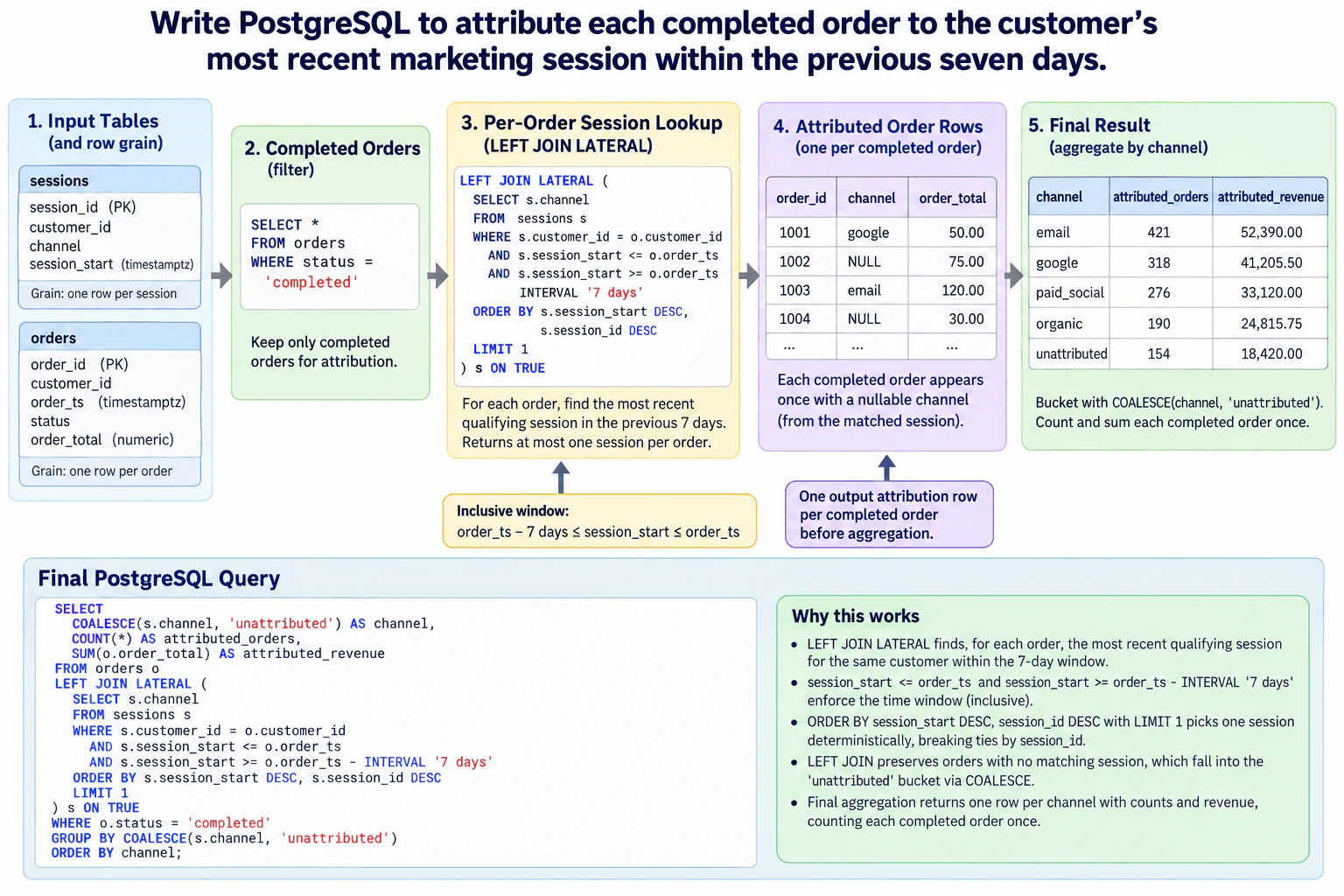
57. Write PostgreSQL to attribute each completed order to the customer’s most recent marketing session within the previous seven days.Sql And DatabasesHard
i Question Details
Use sessions(session_id primary key, customer_id, channel, session_start timestamptz) and orders(order_id primary key, customer_id, order_ts timestamptz, status, order_total numeric). Assign at most one session per completed order, require session_start <= order_ts and no more than seven days earlier, break equal timestamps by session_id, and return channel, attributed_orders, and attributed_revenue, including an unattributed bucket.
Short Interview Answer (30-60 seconds)
I would keep completed orders, then use LEFT JOIN LATERAL to find at most one qualifying session for each order. The lookup matches the same customer, requires session_start to be between order_ts minus seven days and order_ts inclusive, sorts by session_start descending and session_id descending, and keeps LIMIT 1. LEFT JOIN preserves orders with no qualifying session. Finally, COALESCE puts a missing channel into the unattributed bucket, and GROUP BY returns attributed order count and revenue by channel.
The task is to assign each completed order to no more than one marketing session. A customer may have several sessions before an order, so directly joining all eligible sessions could duplicate the order and overstate both order count and revenue. For each order, the query therefore finds only the newest session for the same customer inside the inclusive seven-day lookback window. Equal session timestamps are resolved with session_id. If no session qualifies, the order remains in the result and is grouped into the unattributed bucket.
Useful Questions to Ask the Interviewer
If a qualifying session has channel = NULL, should it also be reported as unattributed, or should it use a separate unknown-channel bucket?
Is the completed status stored exactly as 'completed'?
Should a session exactly seven days before order_ts be eligible? The stated requirement indicates yes.
Can order_total be NULL, and if so, should attributed revenue follow normal SUM behavior or treat NULL as zero?
How to Explain It in an Interview
Start with the data grain. sessions has one row per marketing session because session_id is its primary key. orders has one row per order because order_id is its primary key. Before the final aggregation, the required attribution grain is exactly one row per completed order. The final output grain is one row per channel, including unattributed.
The query keeps only orders whose status is 'completed'. For each such order, LEFT JOIN LATERAL performs a correlated lookup into sessions using the current order's customer_id and order_ts. The conditions s.session_start <= o.order_ts and s.session_start >= o.order_ts - INTERVAL '7 days' implement the inclusive boundary shown in the approved diagram: order_ts - 7 days <= session_start <= order_ts.
The eligible sessions are sorted by s.session_start DESC so the newest session comes first. If two eligible sessions have the same timestamp, s.session_id DESC gives a deterministic tie-break that matches the approved diagram. LIMIT 1 then guarantees that the lateral subquery contributes at most one session row for each order. That prevents the one-to-many relationship from multiplying an order and double-counting its revenue.
LEFT JOIN is required because an INNER JOIN would remove completed orders that have no qualifying session. When the lateral lookup finds no row, the joined session columns are NULL. COALESCE(s.channel, 'unattributed') maps that missing channel to the unattributed bucket. Consistent with the diagram, this expression also maps a matched session whose channel itself is NULL into the same bucket; if that distinction matters, it should be clarified with the interviewer.
The final GROUP BY changes the grain from one attributed row per completed order to one row per channel. COUNT() returns attributed_orders, and SUM(o.order_total) returns attributed_revenue. The result therefore counts every completed order once, including orders without an eligible session.
For validation, first inspect the per-order attribution before aggregation. Its row count should equal the number of completed orders, and no order_id should occur more than once. Test the exact lower boundary, a session at the same timestamp as the order, multiple qualifying sessions, equal session timestamps, and an order with no qualifying session. Then reconcile SUM(attributed_orders) with the number of completed orders and SUM(attributed_revenue) with SUM(order_total) over completed orders, accounting for normal SQL NULL behavior if order_total is nullable.
For performance, the lateral lookup is repeated conceptually for each order, so a useful access path on sessions can matter on large tables. An index beginning with customer_id and supporting the session_start and session_id ordering can reduce lookup work, but index choices should be validated with actual data distribution and EXPLAIN. This is a performance concern, not part of the attribution correctness rule. A ROW_NUMBER solution can also be correct, but LEFT JOIN LATERAL with ORDER BY and LIMIT 1 expresses the required per-order latest-session lookup directly.
Technical Approach
Identify the grains: one row per session, one row per order, then one attribution row per completed order.
Restrict the population to orders where status = 'completed'.
For each order, search sessions having the same customer_id.
Keep only sessions satisfying session_start <= order_ts and session_start >= order_ts - INTERVAL '7 days'.
Sort qualifying sessions by session_start DESC and session_id DESC.
Use LIMIT 1 in a LEFT JOIN LATERAL so each completed order receives at most one session while unmatched orders remain present.
Use COALESCE(s.channel, 'unattributed') for the output channel, matching the approved diagram.
GROUP BY that channel, COUNT() as attributed_orders, and SUM(order_total) as attributed_revenue.
Validate row uniqueness, exact date boundaries, tie handling, order-count reconciliation, and revenue reconciliation.
Practical Complexity & Trade-offs
The query performs one latest-session lookup for each completed order. Without a useful sessions index, those repeated lookups can require substantial scanning as the tables grow. With an appropriate index beginning with customer_id and supporting the session timestamp and tie-break ordering, PostgreSQL can often find the qualifying latest session with much less work. The final aggregation processes the attributed order rows once. The index changes performance, not correctness.
Example
A valid alternative is to LEFT JOIN completed orders to every qualifying session and then use ROW_NUMBER() to rank sessions within each order. Ordering by session_start DESC and session_id DESC gives the same winner rule. Keeping rn = 1 restores one row per completed order before aggregation. This approach is correct but can create a larger intermediate result because all qualifying sessions are joined before ranking, while the lateral LIMIT 1 approach expresses the per-order lookup more directly.
Code
WITH
completed_orders AS (
SELECT
order_id,
customer_id,
order_ts,
order_total
FROM
orders
WHERE
status ='completed'
),
ranked AS (
SELECT
o.order_id,
o.order_total,
s.channel,
ROW_NUMBER() OVER (
PARTITIONBY
o.order_id
ORDERBY
s.session_start DESC,
s.session_id DESC
) AS rn
FROM
completed_orders o
LEFTJOIN sessions s ON s.customer_id = o.customer_id
AND s.session_start <= o.order_ts
AND s.session_start >= o.order_ts -INTERVAL'7 days'
)
SELECTCOALESCE(channel, 'unattributed') AS channel,
COUNT() AS attributed_orders,
SUM(order_total) AS attributed_revenue
FROM
ranked
WHERE
rn =1GROUPBYCOALESCE(channel, 'unattributed')
ORDERBY
channel;
Where it is used
This pattern is common in marketing attribution, campaign reporting, referral analysis, customer-journey analysis, and other event-to-transaction problems where each transaction must be assigned to the latest qualifying event within a fixed lookback period.
Why Interviewers Ask This
This tests whether the candidate can preserve one row per completed order while joining to a one-to-many session history, enforce the required seven-day boundary, choose one latest eligible session deterministically, retain unmatched orders, and aggregate order counts and revenue without duplication.
Common interview mistakes
Using INNER JOIN and dropping unattributed orders; joining all qualifying sessions without reducing to one session per order and therefore double-counting orders or revenue; using a strict greater-than lower bound and excluding a session exactly seven days earlier; failing to make equal timestamps deterministic with session_id; forgetting the completed-order filter; aggregating before resolving the one-session-per-order grain; or assuming COALESCE distinguishes an unmatched session from a matched session whose channel is NULL.
Interview tip
Lead with the grain: one attribution row per completed order before aggregation. Then explain the inclusive seven-day predicates, deterministic ORDER BY, LIMIT 1, and why LEFT JOIN LATERAL preserves unmatched orders. Finish with two checks: completed-order count is preserved and attributed revenue reconciles to completed-order revenue.
Interviewer may ask next
How would you verify that this query does not double-count an order when the customer has several qualifying sessions?
Inspect the attribution result before the final GROUP BY and compare COUNT(*) with COUNT(DISTINCT order_id). They should be equal, and the row count should also equal the number of completed orders. I would test an order with several sessions in the seven-day window, including two sessions with the same session_start, and verify that ORDER BY session_start DESC, session_id DESC with LIMIT 1 selects exactly one deterministic session.
What would change if the business wanted the earliest qualifying session instead of the most recent one?
The customer match, inclusive seven-day predicates, LEFT JOIN LATERAL, and LIMIT 1 can remain the same. I would change the primary ordering to session_start ASC so the earliest qualifying session is first. A deterministic session_id tie-break would still be required, and I would confirm the desired direction for that tie-break if the business rule does not specify it.
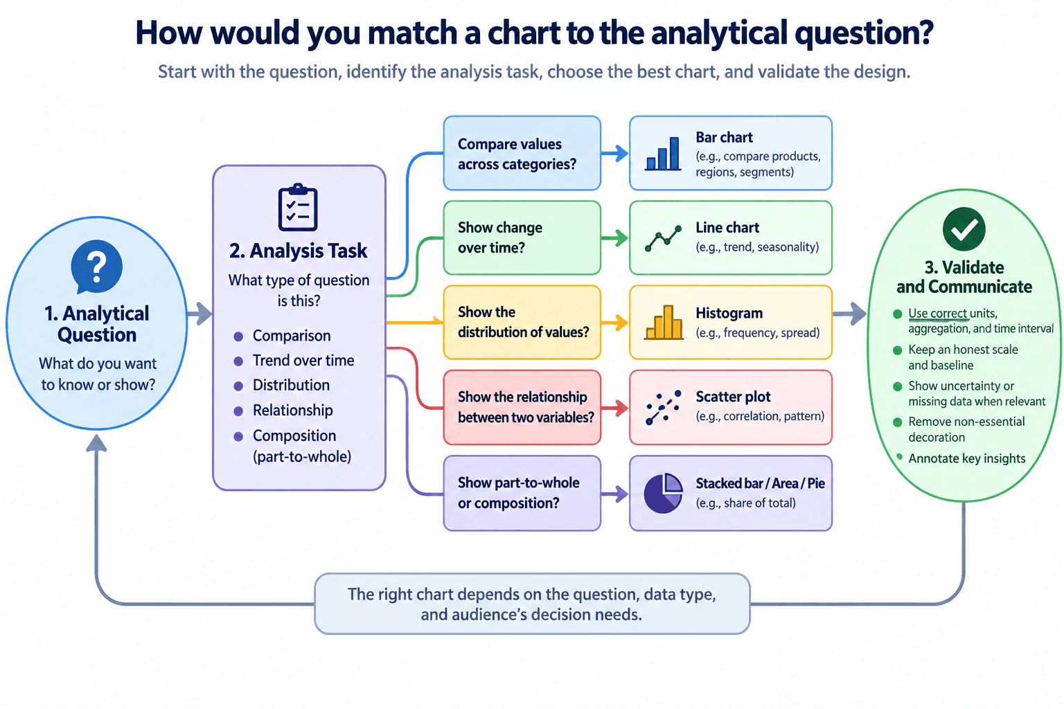
58. How would you match a chart to the analytical question?Data Visualization And StorytellingEasy
i Question Details
Distinguish chart choices for comparison, trend, distribution, relationship, and composition tasks.
Short Interview Answer (30-60 seconds)
I start with the analytical question rather than the chart type. If I am comparing categories, I usually choose a bar chart. For change over time, I use a line chart. For the distribution of one numeric variable, I use a histogram. For the relationship between two numeric variables, I use a scatter plot. For part-to-whole composition, I use a stacked bar, area chart, or pie chart when the parts form a meaningful total. Then I validate units, aggregation, time intervals, scale and baseline, uncertainty, missing data, and accessibility, and I annotate only the evidence that matters to the audience.
Detailed Explanation
The main idea is to choose the chart from the question you are trying to answer, not from personal preference. First identify whether the task is comparison, trend, distribution, relationship, or composition. Then choose a visual whose marks and axes make that pattern easy to see. A bar chart compares categories, a line chart shows change over time, a histogram shows the spread of numeric values, a scatter plot shows how two numeric variables relate, and a stacked bar, area chart, or pie chart can show part-to-whole composition. Finally, validate the chart before presenting it.
Useful Questions to Ask the Interviewer
What decision should the audience make after seeing this chart?
Are we comparing categories, showing change over time, examining a distribution, studying a relationship, or showing composition?
What is the grain of the data, such as one row per customer, transaction, day, or category?
What units, denominators, aggregation rules, and time intervals should be preserved?
Are there missing values, incomplete periods, outliers, or uncertainty that should be shown?
Who is the audience, and how much detail do they need?
How to Explain It in an Interview
I would use a question-first decision process.
Start with the analytical question. I first clarify what the viewer needs to know and what decision the chart should support. That prevents choosing a chart just because it looks familiar or attractive.
2. Classify the analysis task. I map the question to the pattern I need to reveal:
Comparison: compare values across categories.
Trend: show how a value changes over time.
Distribution: show how observations are spread across a numeric range.
Relationship: show whether two numeric variables move together or form a pattern.
Composition: show how parts contribute to a meaningful whole.
Match the chart to that task. For comparison, I would normally use a bar chart because position and length make differences across categories easy to compare. I would preserve consistent units and normally use a zero baseline when bar length represents magnitude.
For trend over time, I would use a line chart because the ordered x-axis and connected points make direction, changes, and possible seasonality visible. I would preserve the actual time interval and avoid hiding missing periods.
For distribution, I would use a histogram for a numeric variable. The bins summarize how often values fall within ranges, helping show frequency, spread, shape, clusters, and possible outliers. Bin width can change the apparent shape, so I would choose and validate it carefully.
For a relationship between two numeric variables, I would use a scatter plot. Each observation is represented by its x and y values, which makes patterns, clusters, unusual observations, and possible association visible. I would not describe correlation as causation without supporting evidence.
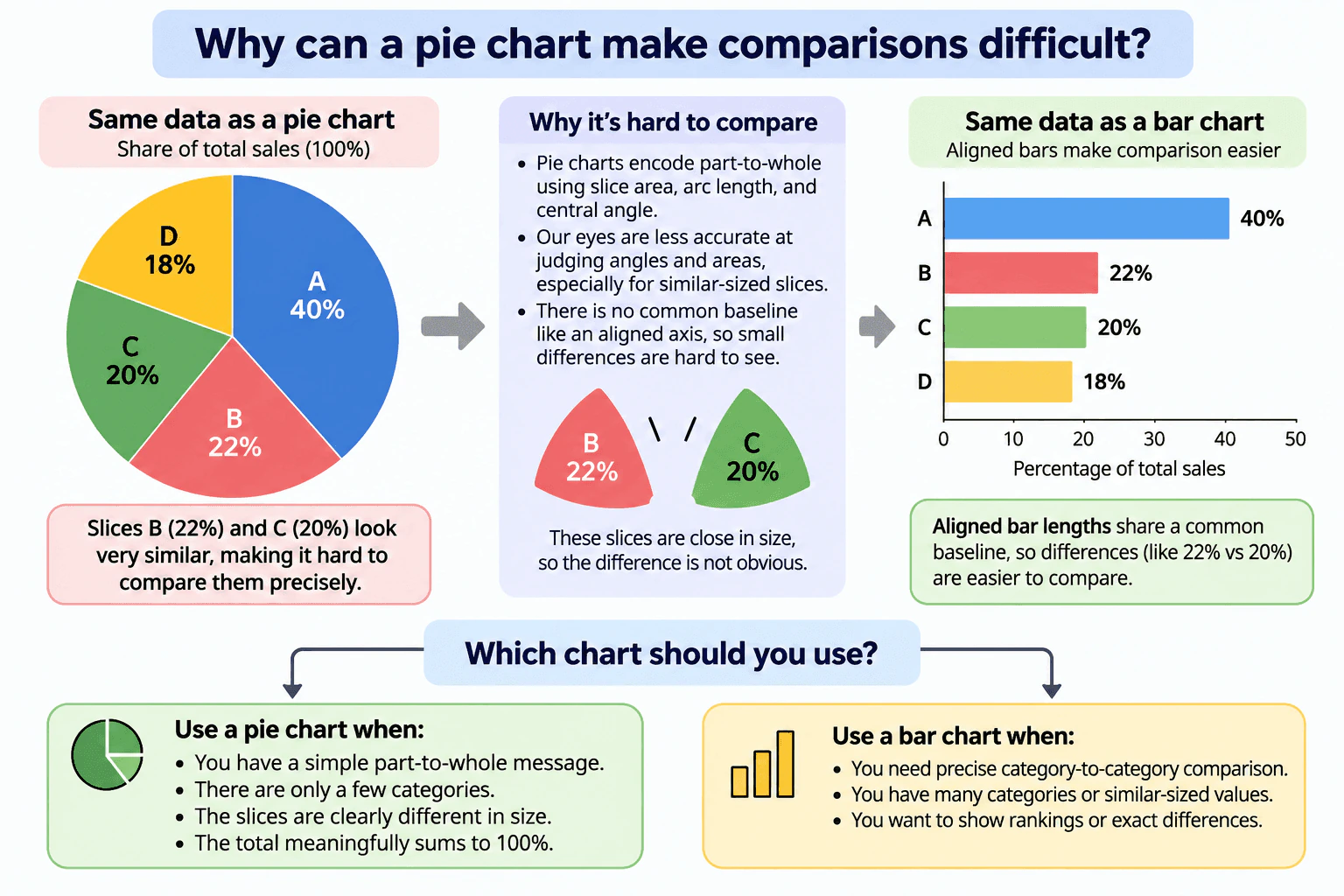
For composition, I would use a stacked bar, area chart, or sometimes a pie chart when the categories are meaningful parts of one total. A stacked bar is often easier when precise comparison matters. An area chart is more appropriate when composition changes across an ordered dimension such as time. A pie chart is best kept to a small number of clearly distinguishable parts when the goal is a simple share-of-total view.
Validate the visual encoding. After choosing the chart, I check that the aggregation, grain, units, denominator, sorting, axis scale, baseline, and time interval agree with the underlying question. I also check whether missing data or uncertainty could change the interpretation. If uncertainty is material, I would represent it rather than imply false precision.
Remove visual elements that do not support the decision. I keep the design simple. Decoration, unnecessary gridlines, excessive colors, redundant labels, or unrelated metrics can distract from the analytical point. Color should carry a clear meaning and should not be the only cue, because accessibility matters.
Annotate the evidence that matters. I would annotate an important change, turning point, outlier, or threshold when it helps explain the conclusion. I would not label every point. The annotation should explain evidence, while the recommendation should remain separate from the observation.
Adapt the final presentation to the audience. An executive audience usually needs the decision, key pattern, material limitation, and implication quickly. An operational audience may need more detailed filters, segments, intervals, or drill-down information. The underlying numbers should remain consistent even if the level of detail changes.
The final principle is that the right chart depends on the analytical question, the data type, and the audience's decision needs. Chart choice is only the first step; truthful scales, consistent units, preserved aggregation, visible uncertainty where material, and focused annotation are what make the visualization defensible.
Technical Approach
State the decision or analytical question.
Identify whether the task is comparison, trend, distribution, relationship, or composition.
Confirm the data types, population, grain, units, aggregation, denominator, and time interval.
Choose the chart: bar for category comparison, line for time trend, histogram for numeric distribution, scatter plot for two-numeric-variable relationships, and stacked bar, area, or pie for meaningful part-to-whole composition.
Check scale, baseline, ordering, missing data, uncertainty, and accessibility.
Remove nonessential visual elements.
Add only decision-relevant annotations.
Validate the chart against the underlying data and adapt the level of detail to the audience.
Practical Insights
Chart selection itself is inexpensive; the main cost is analytical and communication effort. A simple chart is usually faster to build, validate, and understand than a highly customized visual. The important tradeoff is between simplicity and detail: too little detail can hide uncertainty or context, while too much detail can obscure the main pattern. Interactive dashboards may add maintenance and testing work because filters, aggregation, and drill-down behavior must remain consistent.
Why Interviewers Ask This
The interviewer is testing whether I can translate an analytical question into a visual that represents the comparison truthfully, preserves the data's grain, units, scale, and time structure, and communicates the result clearly enough for the audience to make a decision.
Common interview mistakes
Common mistakes include choosing a chart before defining the question, using a line chart for unordered categories, using a pie chart when categories do not form a meaningful whole, using too many pie slices, hiding missing time periods, using misleading axis scales, truncating bar-chart baselines in a way that exaggerates differences, mixing units or aggregation levels, implying causation from a scatter plot, ignoring histogram bin sensitivity, relying only on color, adding decorative elements that distract from the decision, and annotating conclusions more strongly than the evidence supports.
Interview tip
Explain chart choice as a decision process, not a memorized list: name the analytical task, choose the visual that best exposes that pattern, then state how you would validate scale, units, aggregation, uncertainty, and audience needs.
Interviewer may ask next
What would you do if the analytical question suggests one chart type, but missing data or irregular time intervals could make that chart misleading?
I would keep the analytical objective but change how I prepare or present the visual. For a time trend, for example, I would preserve the actual time intervals, show gaps instead of silently connecting missing periods when that connection would imply observations that do not exist, and annotate material missingness. I would also check whether aggregation to a coarser interval is defensible. The chart should reveal the available evidence without creating continuity, precision, or completeness that the data does not support.
How would your chart choice change if the audience needs precise comparisons rather than a quick high-level story?
I would favor encodings that support precise comparison. For example, I would prefer a bar chart over a pie chart for comparing category magnitudes because aligned positions and lengths are easier to compare accurately. For composition across several groups, I might use stacked bars, or separate bars if comparing individual components is more important than emphasizing the total. I would still keep the design simple, but I would include the units, scale, sorting, relevant labels, and any necessary detail that helps the audience make an accurate comparison.
59. Why can a pie chart make comparisons difficult?Data Visualization And StorytellingEasy
i Question Details
Discuss similar-sized pie slices and when a simple part-to-whole split remains appropriate.
Short Interview Answer (30-60 seconds)
A pie chart can make comparisons difficult because people must judge differences in slice angles, areas, and arc lengths. When two slices are close in size, such as 22% and 20%, the difference can be hard to see accurately. A bar chart is usually better for precise category-to-category comparison because the bars share a common baseline and their lengths are easier to compare. I would still use a pie chart for a simple part-to-whole message with only a few categories, clearly different slice sizes, and a meaningful total of 100%.
Detailed Explanation
A pie chart shows how categories make up one whole, but it is not always good for comparing categories precisely. The viewer must compare slice angles, areas, and arc lengths instead of positions along a shared scale. This becomes difficult when slices are close in size. For example, the diagram shows 22% and 20%; those slices look very similar. A bar chart makes that difference easier to judge because all bars begin from the same baseline. A pie chart still works when the message is a simple part-to-whole split with only a few clearly different categories.
Useful Questions to Ask the Interviewer
Is the main goal to show composition of a whole or to compare categories precisely?
Do all categories add up to one meaningful total, such as 100%?
Are there only a few categories, or are several values close in size?
Does the audience need exact ranking or only a quick part-to-whole message?
How to Explain It in an Interview
Start with the analytical question. If the audience needs to understand how a small number of categories contribute to one meaningful total, a pie chart can be appropriate. Each slice represents a proportion of that whole.
The limitation is the visual encoding. With a pie chart, the viewer compares slices mainly through central angle, area, and arc length. People are less precise at judging small differences with these encodings than at comparing aligned lengths or positions. That is why similar-sized slices can look almost the same.
The diagram illustrates this with categories A, B, C, and D representing 40%, 22%, 20%, and 18% of total sales. The important comparison is between B at 22% and C at 20%. In the pie chart, those two slices are visually close, so the 2-percentage-point difference is not obvious. The same values shown as horizontal bars are easier to compare because each bar starts from the same baseline and uses a consistent percentage scale.
So I would choose a bar chart when the goal is precise category-to-category comparison, ranking, or distinguishing similar-sized values. I would use a pie chart when there are only a few categories, the total meaningfully sums to 100%, the slices are clearly different in size, and the main message is composition rather than exact comparison.
I would also validate that the categories are mutually exclusive parts of the intended whole, use the same denominator, and collectively account for that whole. The chart should not imply a part-to-whole relationship if categories overlap or do not form one complete total. I would keep units and labels consistent, avoid unnecessary decoration, and use text labels or other redundant cues so the interpretation does not depend on color alone.
The final decision is therefore based on the comparison the audience needs to make: use a pie chart for a simple, high-level part-to-whole story, but prefer an aligned bar chart when accuracy of comparison matters.
Technical Approach
Identify whether the task is part-to-whole communication or precise category comparison.
Confirm that the categories use one consistent denominator and form a meaningful whole if considering a pie chart.
Check the number of categories and whether several shares are similar in size.
Use a pie chart only for a small, simple composition with clearly different slices.
Use a bar chart when precise comparison, ranking, or similar-sized values matter.
Keep labels, units, scale, and percentage definitions consistent.
Validate that the chosen visual supports the audience's decision without misleading emphasis.
Practical Insights
There is no meaningful computational complexity for this chart-choice question. The main tradeoff is communication accuracy versus simplicity. A pie chart can communicate a simple composition quickly, while a bar chart uses a common axis and baseline that make small differences and rankings easier to compare accurately.
Why Interviewers Ask This
Interviewers want to see whether you understand that chart choice should follow the comparison being made. A strong Data Analyst should recognize that pie charts are useful for simple part-to-whole communication but are weaker when the audience needs to compare similar values precisely. The judgment is knowing when to keep the pie chart and when to switch to a bar chart with a common baseline.
Common interview mistakes
Using a pie chart when categories do not form one meaningful whole; using too many slices; expecting viewers to distinguish very similar slice sizes precisely; relying only on color to identify slices; omitting the denominator or unit; and choosing a pie chart for ranking when an aligned bar chart would communicate the comparison more clearly.
Interview tip
State the comparison first. Say that pie charts are good for a simple part-to-whole message, but aligned bars are better when the interviewer asks about precise differences, similar-sized values, or ranking. Use the 22% versus 20% example to make the reasoning concrete.
Interviewer may ask next
What would you check before deciding that a pie chart is appropriate for a part-to-whole view?
I would confirm that the categories are mutually exclusive parts of one meaningful whole, use the same denominator, and collectively sum to the intended whole, such as 100%. I would also check that there are only a few categories and that their sizes are different enough to read easily. If categories overlap, do not form one complete whole, or are very similar in size, I would choose another chart such as a bar chart.
What would you do if the audience wants both the overall composition and precise comparison between similar categories?
I would prioritize the decision the audience needs to make. If precise comparison matters, I would use a bar chart with a common baseline and percentage labels because it makes small differences easier to judge. I could still explain that the percentages represent parts of the same whole in the title or an annotation instead of relying on a pie chart to communicate both composition and precision.
60. How would you use chart colors accessibly?Data Visualization And StorytellingEasy
i Question Details
For accessible chart colors, address ordered values, categories, contrast, and alternatives to color-only distinctions.
Short Interview Answer (30-60 seconds)
I first ask what color is encoding. For ordered values, I use a sequential light-to-dark scale so the visual order matches low-to-high values. For categories, I use distinct hues, but I also add redundant cues such as direct labels, marker shapes, line styles, or patterns. I keep text and important marks clearly contrasted with the background and avoid low-contrast combinations. Finally, I test whether the chart still makes sense in grayscale and under common color-vision deficiencies. Color can reinforce meaning, but it should not be the only way the audience understands the chart.
Detailed Explanation
Accessible chart color means choosing color so people can understand the same message even if they perceive colors differently. I start by asking what the color represents. Ordered values need a visual order, so a sequential light-to-dark scale works well. Categories need separation, so I use distinct hues. In both cases, I keep important text and marks clearly contrasted with the background. I never depend on color alone: labels, shapes, line styles, or patterns should repeat the meaning. Finally, I check the chart in grayscale and with common color-vision-deficiency simulations before publishing.
Useful Questions to Ask the Interviewer
Is color representing an ordered value or separate categories?
Which chart elements must remain distinguishable if the viewer cannot perceive the colors?
Will the chart be viewed on a light background, dark background, screen, or printed page?
Are there brand colors or design constraints that I need to work within?
Does the audience need to compare precise values, identify categories, or recognize a low-to-high pattern?
How to Explain It in an Interview
I would explain the process as a simple flow from meaning to encoding to validation.
First, I determine what color encodes. If the values have a natural order, such as low to high, I use a sequential palette. The diagram shows this as a light-to-dark progression: lighter shades represent lower values and darker shades represent higher values. The important point is that the visual progression should communicate the ordering clearly.
If color represents categories with no natural order, I use distinct hues. I do not rely on those hues alone. As shown in the diagram, a line chart can also give each series a different marker shape and line style: for example, a circle with a solid line, a square with a dashed line, and a triangle with a dotted line. Direct labels can also reduce dependence on a color legend.
Next, I check contrast. Important chart marks, labels, axes, and supporting text should be clearly distinguishable from the background. A dark mark on a light background, or a light mark on a dark background, is generally easier to read than a low-contrast combination. I also avoid assuming that two colors are distinguishable simply because they look different to me.
Then I make the chart understandable without color. If removing color destroys the meaning, the design is too dependent on color. I can reinforce the same information with direct labels, shapes, line styles, patterns, position, or readable text. These extra cues should support the message rather than add unnecessary decoration.
Finally, I validate the chart. I review it in full color, grayscale, and common color-vision-deficiency simulations. I check whether ordered values still look ordered, categorical series can still be identified, labels remain readable, and the main message is still clear. If an important distinction disappears, I revise the palette or strengthen the non-color cue.
The main tradeoff is that redundant cues can make a chart slightly busier. I would therefore use only the minimum extra cues needed for reliable identification. The goal is not to remove color. The goal is to make color useful while keeping the chart understandable when color alone is not enough.
Technical Approach
Identify what the color represents: ordered values or categories.
For ordered values, use a sequential light-to-dark progression that preserves the low-to-high order.
For categories, use distinct hues and keep category assignments consistent.
Add redundant cues such as direct labels, marker shapes, line styles, or patterns so color is not the only distinction.
Check that important text, marks, axes, and labels have sufficient contrast with the background.
Review the chart in grayscale to confirm that the main distinctions remain understandable.
Test common color-vision-deficiency views and revise confusing combinations.
Remove unnecessary decoration and retain only cues that support the audience's understanding.
Practical Insights
There is usually little computational cost; the main cost is design and validation time. Adding shapes, patterns, labels, and line styles can make the chart more accessible, but too many cues can create clutter. The best balance is to use a restrained set of colors and add only enough redundant encoding to keep every important series, category, or state identifiable without relying on color alone.
Why Interviewers Ask This
Interviewers want to know whether I can use color as a meaningful visual encoding without excluding people who have color-vision deficiencies or low vision. A strong answer should distinguish ordered values from categories, use sufficient contrast, avoid color-only communication, and explain how the final chart would be validated.
Common interview mistakes
Common mistakes include using unrelated rainbow-like colors for ordered values, assigning similar hues to separate categories, using low-contrast text or marks, depending on red versus green as the only signal, giving each series a color but no other identifying cue, and assuming a chart is accessible because it looks clear to its creator. Another mistake is adding so many patterns, markers, and labels that the chart becomes unnecessarily crowded.
Interview tip
Structure the answer around four ideas: ordered values, categories, contrast, and alternatives to color-only distinctions. Finish by explaining that you would validate the chart in grayscale and with color-vision-deficiency simulations. That shows both design judgment and a practical verification step.
Interviewer may ask next
What would you do if several categorical series still looked similar after a color-vision-deficiency check?
I would strengthen the redundant encoding instead of relying on additional colors alone. For example, I could give each line a different marker shape and line style, add direct labels near the series, or use patterns where appropriate. I would then repeat the grayscale and color-vision-deficiency checks. The goal is for every category to remain identifiable even when its hue is difficult to distinguish.
What if brand guidelines require colors that are difficult to distinguish or do not provide enough contrast?
I would keep the brand colors where they do not carry critical meaning, but I would not let branding make the data ambiguous. I could pair those colors with readable labels, stronger foreground-background contrast, marker shapes, line styles, patterns, or outlines. If an important label or mark still cannot be read clearly, I would use an approved accessible variation rather than relying on the problematic color alone.
More questions load as you scroll
Disclaimer: This interview guide is for educational and informational purposes only. It is designed to help readers prepare, but it does not guarantee any interview result, hiring decision, offer, or outcome. Interview questions, hiring criteria, and preferred answers can vary by employer, interviewer, industry, location, and time. All answers, examples, and explanations in this guide are suggested examples for interview preparation, not definitive answers or instructions for professional practice. They are based on research and judgment, are provided without warranties of any kind, and should be adapted to the question, role, and applicable laws and professional requirements. Diagrams are simplified illustrations intended to highlight the main concepts and their relationships; actual situations, systems, and practices may be more complex. Alternative approaches may be equally valid or better suited to a particular question, context, or interviewer. To the fullest extent permitted by applicable law, the contributors and publisher are not liable for decisions made, actions taken, or losses incurred based on this guide.
State Laws and Professional Responsibilities: Laws and requirements governing an occupation vary by state and jurisdiction. You are responsible for checking the current laws, licensing requirements, and scope-of-practice rules that apply to your location and role, and for ensuring that your answers and actions comply with them. Adapt examples in this guide to those requirements. This guide is not legal advice.
Content Accuracy and Verification: To the fullest extent permitted by applicable law, we do not represent or warrant that interview guides, questions, answers, examples, or diagrams are accurate, complete, current, error-free, or suitable for any particular purpose. You are responsible for independently reviewing and verifying the information before relying on it.