188 Data Scientist Interview Questions & Answers

92 top • 12 Amazon • 15 Apple • 13 Google • 12 Meta • 15 Microsoft • 15 Netflix • 14 NVIDIA

Data Scientist icon

Questions with Detailed ExplanationsWith Detailed Explanations

(Last Updated: September 8, 2026)

1. What is machine learning, and how does it differ from rule-based programming?Machine LearningEasy

Question Details

Define machine learning in terms of learning patterns from data to make predictions or decisions. Contrast it with software whose behavior is specified through explicit rules, then give one realistic Data Scientist use case for each approach and explain when a hybrid design is preferable.

Short Interview Answer (30-60 seconds)

Machine learning learns a mapping from historical data and uses it to predict or decide for new cases. Rule-based software instead executes explicit if-then logic written by people. I would use ML for customer churn prediction, rules for defined lending-policy constraints, and a hybrid when learned predictions must still obey mandatory business, compliance, or safety rules.

Detailed Explanation

Machine learning learns patterns from observed data so a system can make predictions or decisions for new cases. We start with a population or real-world process, collect observations, represent each case with features X, and, for supervised learning, define a target or label y. Training learns a model f that maps X to y and should generalize beyond the training examples. Rule-based programming works differently: people explicitly write the decision logic, such as if-then conditions, and the software applies those rules exactly as written.

Useful Questions to Ask the Interviewer
  1. Do we have historical examples from which a useful pattern can be learned?
  2. Are any business, compliance, or safety constraints mandatory and therefore better represented as explicit rules?
  3. Is the relationship simple and stable enough for hand-written logic, or is it noisy, high-dimensional, or pattern-rich?
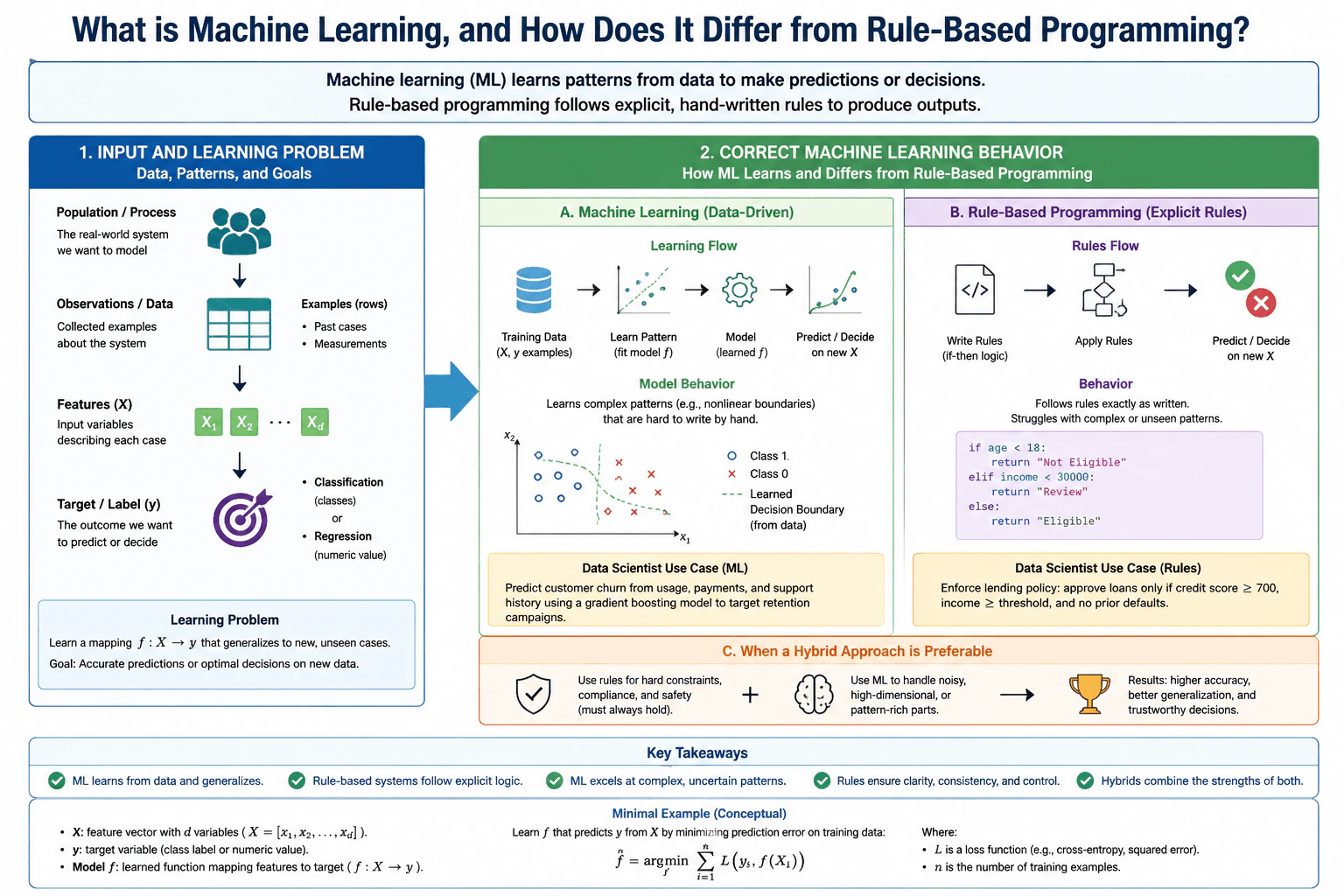
What is machine learning, and how does it differ from rule-based programming? diagram
How to Explain It in an Interview

Start with the input and learning problem. The population is the real-world process we want to model. Observations are collected examples from that process. Each example is described by features X, which are the input variables. In supervised learning, the target or label y is the outcome we want to predict or the decision-related quantity we want the model to estimate.

Machine learning uses training data containing examples such as X and y. A learning algorithm fits a model f from those examples. Conceptually, training chooses a function that reduces prediction error on the training data, for example by minimizing a loss function L. After training, the learned model receives a new feature vector X and produces a prediction or decision. For classification, the learned model may create a decision boundary that separates classes based on patterns found in the data rather than boundaries manually specified by a developer.

A realistic Data Scientist use case is customer churn prediction. Historical customer examples can contain features such as usage, payment behavior, and support history. A model can learn combinations of these signals and predict churn risk for new customers. This is a good machine-learning problem because the useful relationships may be noisy, high-dimensional, nonlinear, or difficult to express as a manageable set of hand-written conditions. The model still needs evaluation on unseen data because low training error does not guarantee good generalization.

Rule-based programming has a different flow. A person with domain knowledge writes explicit rules, the program applies those rules to the current inputs, and the rules directly determine the output. For example, a lending-policy system may contain explicitly defined requirements such as a minimum credit score and minimum income threshold. Those policy constraints can be encoded directly as if-then logic. The result is deterministic for the same inputs and the decision path is usually straightforward to audit.

The important distinction is where the decision behavior comes from. In machine learning, the predictive relationship is learned from data. In rule-based programming, the relationship is specified explicitly by people. Machine learning is strong when many interacting signals create complex or uncertain patterns. Rule-based systems are strong when logic is known in advance, must be followed exactly, or needs direct control and traceability.

Each approach also has limitations. A learned model depends on the quality and relevance of its training data and can perform poorly on cases that differ from what it learned. A rule-based system can struggle when the problem has many exceptions, subtle interactions, or unseen patterns because those behaviors must be anticipated and coded manually. Large rule sets can also become difficult to maintain.

A hybrid approach is preferable when both types of behavior are needed. Explicit rules can enforce hard constraints for business policy, compliance, or safety, while machine learning handles the noisy, high-dimensional, pattern-rich part of the problem. For example, an ML model may provide a score or prediction, while mandatory rules determine whether that prediction can be acted on. The combined system can offer learned flexibility together with explicit control, but it should not be assumed to produce higher accuracy or better business outcomes without evaluation.

Technical Approach
  1. Define the real-world population or process and the prediction or decision that is needed.
  2. Identify the observations and features X available for each case.
  3. If supervised learning is appropriate, define the target y and collect historical training examples.
  4. Use machine learning when useful behavior must be learned from complex or pattern-rich data; train a model f: X → y and evaluate it on unseen data.
  5. Use explicit rules when the required behavior is already known, deterministic, and directly expressible as if-then logic.
  6. Identify hard business, compliance, or safety constraints that should always hold.
  7. Use a hybrid design when a learned model should handle complex patterns while explicit rules enforce those mandatory constraints.
Practical Insights

Machine learning has data, training, evaluation, and monitoring costs. Its benefit is that it can learn complicated patterns without manually coding every condition. Rule-based software usually needs less model infrastructure and its logic is easier to trace, but many interacting rules can become difficult to write, test, and maintain. A hybrid system adds integration and testing work because both the model and the rules must behave correctly together. Machine learning also has statistical uncertainty: fitting historical examples well does not guarantee good behavior on new or shifted data.

Why Interviewers Ask This

Interviewers want to verify that a Data Scientist understands the fundamental difference between behavior learned from data and behavior explicitly programmed by people. They also want practical judgment about choosing between machine learning, deterministic rules, and a hybrid design instead of assuming that machine learning is always the best solution.

Common interview mistakes

One mistake is saying that machine learning simply means software without rules. The key distinction is that the predictive mapping is learned from data rather than fully specified through hand-written decision logic. Another mistake is assuming machine learning is always better; explicit, stable policies are often better represented directly as rules. A third mistake is assuming good performance on training data means the model will generalize to new cases. Another mistake is saying rule-based systems can never handle complex logic; they can, but large and exception-heavy rule sets may become difficult to maintain. Finally, do not claim that a hybrid automatically improves accuracy, generalization, or business results.

Interview tip

Start with the simplest contrast: machine learning learns predictive behavior from data, while rule-based software executes behavior explicitly written by people. Then walk through one example of each and finish with the hybrid case: use ML for complex patterns and rules for constraints that must always hold.
Interviewer may ask next
What if the historical data for the customer churn model is limited or does not represent the new customers well?

Then I would be cautious about relying on the learned model. Machine learning can only learn patterns supported by its training examples, so limited or unrepresentative data can cause poor generalization. I would evaluate the model on separate unseen data that reflects the intended population and compare its behavior with a simpler baseline. If the evidence is weak, explicit rules or a more limited hybrid design may be safer until better data is available.

What happens if the machine-learning prediction conflicts with a mandatory lending-policy rule in a hybrid system?

The mandatory rule should take precedence when it represents a hard business, compliance, or safety constraint. The machine-learning model can provide a score or recommendation based on learned patterns, but it should not override a condition that the system is required to enforce. The final decision flow should therefore use the model where statistical judgment is useful and then apply the required rule constraints before producing the final outcome.

2. How do supervised and unsupervised learning differ?Machine LearningEasy

Question Details

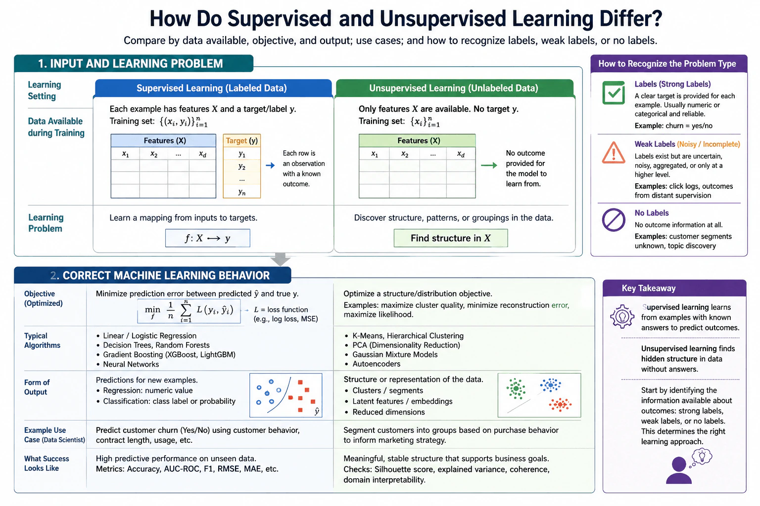
Compare the two learning settings in terms of the data available during training, the kind of objective being optimized, and the form of output produced. Give one Data Scientist use case for each, and explain how you would recognize that a proposed problem has labels, weak labels, or no labels.

Short Interview Answer (30-60 seconds)

Supervised learning uses features plus known labels and learns to predict a target, such as customer churn. Unsupervised learning has features but no target and discovers structure, such as customer segments. Strong labels are clear outcomes, weak labels are noisy or incomplete signals, and no-label problems have no outcome information.

Detailed Explanation

Supervised and unsupervised learning mainly differ in what information is available during training and what the algorithm is asked to learn. In supervised learning, each training example contains features X and a target y. The model learns a mapping from X to y and produces predictions. In unsupervised learning, only features X are available. There is no target y, so the method searches for useful structure, patterns, groups, or representations. The practical first step is therefore to determine whether the proposed problem has reliable labels, weak labels, or no labels.

Useful Questions to Ask the Interviewer
  1. Is there a target or outcome recorded for each training example?
  2. If a target exists, is it a reliable direct label or a noisy, incomplete, aggregated, or proxy signal?
  3. Is the goal to predict a known outcome or to discover structure in the feature data?
  4. What form of output is useful: a prediction, a customer segment, or another learned representation?
  5. If labels exist, how and when were they created relative to the features available to the model?
How do supervised and unsupervised learning differ? diagram
How to Explain It in an Interview

Start with the training data. In supervised learning, a training example contains features X and a target y. The target is the answer the model is trying to predict. For example, customer behavior, contract length, and usage can be features, while churn yes/no can be the target. The model learns a function from X to y.

The supervised objective measures prediction error against the known target. For regression, an objective can minimize mean squared error. For classification, it can minimize a classification loss such as cross-entropy. The important point is that the target is available during training, so the model can compare its prediction with the known answer and update its parameters to reduce loss.

The output from supervised learning is normally a prediction for a new example. Regression produces a numeric value. Classification can produce a class label or probability. Common supervised model families include linear regression, logistic regression, decision trees, random forests, gradient boosting, and neural networks. The defining property is not the specific algorithm; it is that labeled training examples are available.

A Data Scientist use case is predicting whether a customer will churn. The training data contain customer features and a known churn outcome. On unseen labeled data, predictive quality can be evaluated with metrics appropriate to the task, such as accuracy, AUC-ROC, or F1 for classification, or RMSE and MAE for regression.

In unsupervised learning, the training data contain X but no target y. The method cannot minimize prediction error against a known answer because no answer is supplied. Instead, it optimizes an objective related to structure or distribution in X. For example, k-means minimizes within-cluster variation, PCA finds directions that explain variance, an autoencoder can minimize reconstruction error, and probabilistic models can maximize likelihood.

The output is therefore usually discovered structure or a learned representation rather than a prediction of a supplied target. Examples include clusters or customer segments, latent features or embeddings, and reduced-dimensional representations. Common unsupervised methods include k-means, hierarchical clustering, PCA, Gaussian mixture models, and autoencoders.

A Data Scientist use case is customer segmentation. If purchase behavior is available but there is no predefined segment label, an unsupervised method can group customers with similar patterns. The result can support analysis or marketing strategy, but the clusters are discovered by the method rather than learned from known segment answers. Their usefulness can be examined through measures such as silhouette score when appropriate, explained variance for dimensionality reduction, stability across reasonable changes, and domain interpretability. These checks do not create ground-truth labels that were absent during training.

To recognize the learning setting, inspect the outcome information. Strong labels mean there is a clear, reasonably reliable target for individual examples, such as churn yes/no. Weak labels are outcome signals that exist but are noisy, incomplete, aggregated, or created indirectly from proxy information. They can still provide supervision, but they should not be treated as perfectly reliable ground truth. No labels means there is no target information at all. If the goal is then to find patterns, groups, or representations in X, the problem is naturally unsupervised.

Weak labels should not automatically be confused with semi-supervised learning. Weak labeling describes label quality. Semi-supervised learning describes a training setup that combines labeled and unlabeled examples. Those ideas can overlap, but they are not the same concept.

The key distinction is simple: supervised learning learns from examples with target information to predict outcomes, while unsupervised learning learns from data without target labels to discover structure.

Technical Approach
  1. Identify what one training example or row represents.
  2. Separate the available features X from any proposed outcome y.
  3. Check whether y is available for the training examples.
  4. If a clear target y exists, treat the task as supervised and define the prediction output and a loss that compares predictions with known targets.
  5. If target information exists but is noisy, incomplete, aggregated, or proxy-based, treat it as weak labeling and assess its reliability before using it as supervision.
  6. If no target exists and the goal is to discover groups, representations, or patterns, treat the task as unsupervised.
  7. Match evaluation to the setting: prediction metrics on unseen labeled data for supervised learning, and structure, stability, representation quality, or domain usefulness for unsupervised learning.
Practical Insights

Supervised learning needs labeled examples, and obtaining reliable labels can require time and cost. Its advantage is that predictions can be checked directly against known outcomes on unseen labeled data. Unsupervised learning does not require target labels, but its results can be harder to judge because there may be no single correct cluster or representation. Different features, scaling choices, algorithms, and hyperparameters can produce different structures. Weak labels provide some target information but add uncertainty because the signal may be noisy or incomplete.

Why Interviewers Ask This

This question tests whether a Data Scientist can identify what information is available during training and choose the correct learning setting. A strong answer distinguishes features from labels, explains how the objective changes when a target is absent, describes the different forms of output, and recognizes strong labels, weak labels, and unlabeled data without treating every dataset as a prediction problem.

Common interview mistakes

Common mistakes are saying that supervised learning means only classification, even though regression is also supervised; saying that unsupervised learning has no objective, even though methods such as k-means, PCA, autoencoders, and probabilistic models optimize defined objectives; treating discovered clusters as proven ground-truth categories; evaluating an unsupervised problem as if true labels necessarily existed; treating noisy or proxy labels as perfectly reliable; and confusing weak labels with semi-supervised learning. Another mistake is deciding from an algorithm name instead of first checking what training information and target signal are actually available.

Interview tip

Organize the answer around three contrasts: training data, objective, and output. Then give one matching use case for each setting and finish by explaining strong labels, weak labels, and no labels. This keeps the answer clear and directly aligned with the question.

Interviewer may ask next
If the churn signal exists but is noisy or incomplete, is the problem still supervised learning?

It can still provide supervision, but I would describe the churn signal as a weak label rather than perfect ground truth. I would first understand how the labels were created, how much is missing, and how reliable the signal is. A supervised method may still be appropriate, but training and evaluation should account for label quality. Weak labels describe unreliable supervision; they do not by themselves mean the setup is semi-supervised.

What would you do if customer segmentation produces different clusters when the data or clustering settings change?

I would treat that as evidence that the discovered structure may be unstable. I would test stability across reasonable data samples and modeling choices, inspect separation measures such as silhouette score when appropriate, and check whether the segments remain interpretable and useful for the intended analysis. If small changes produce completely different groups, I would be cautious about treating those clusters as meaningful categories.

3. How does logistic regression produce a classification probability?Machine LearningEasy

Question Details

Explain the binary-classification setting with one row per observation, a binary target, numeric feature inputs available at prediction time, and a linear score transformed into a probability. Discuss the role of the link function, the decision threshold, coefficient interpretation, and the assumptions that can make probability estimates unreliable.

Short Interview Answer (30-60 seconds)

Logistic regression computes a linear score from the features. The logit link says that score represents log-odds, and the inverse link, the sigmoid, maps it to a probability between 0 and 1. That gives P(y = 1 | x). A separate threshold, such as 0.5, can then turn the probability into a class prediction.

Detailed Explanation

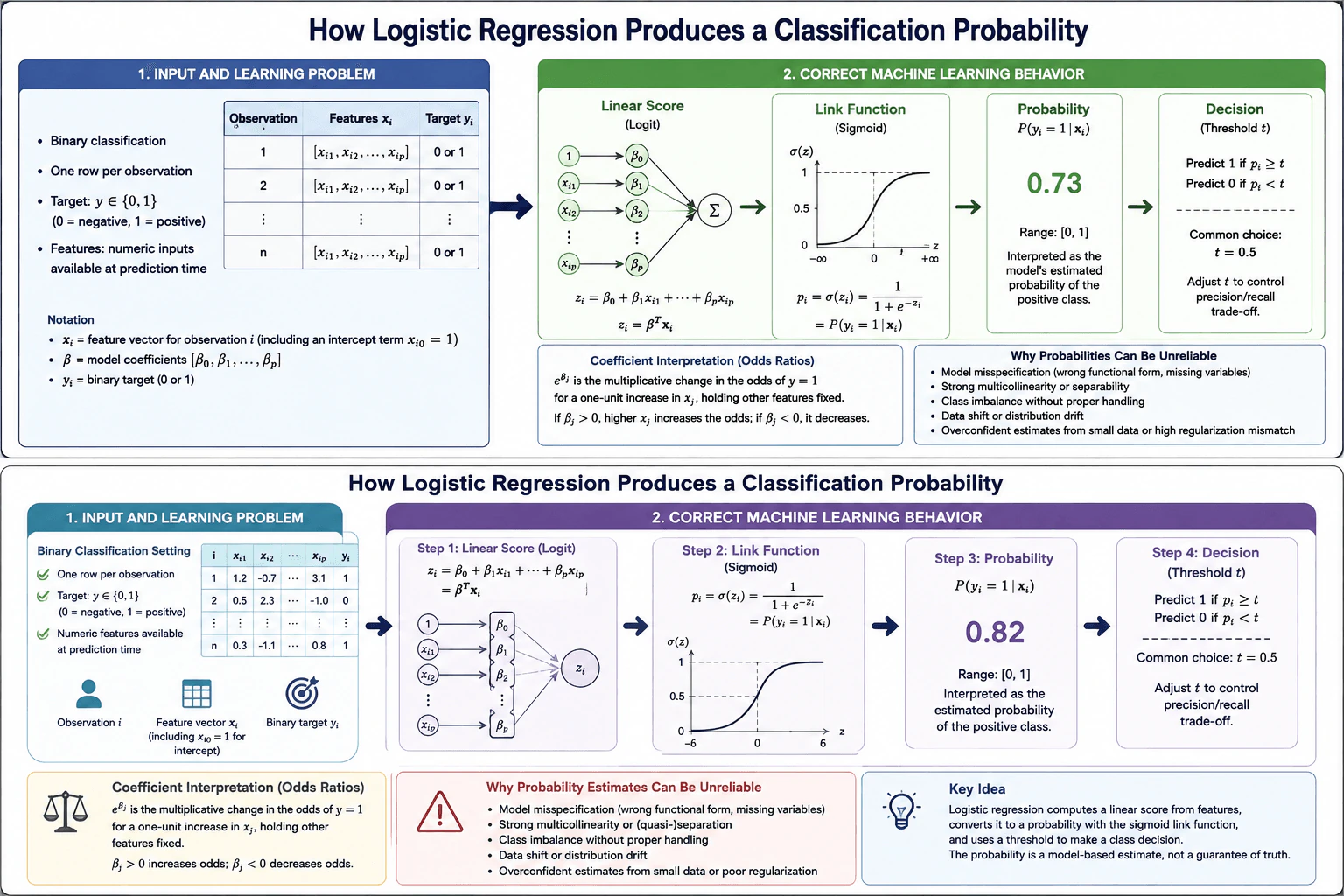
In binary classification, each observation is one row with numeric features available when prediction is made and a target y that is either 0 or 1. Logistic regression combines those features into a linear score, z = β0 + β1x1 + ... + βpxp. The model treats this score as the log-odds of the positive class. Because z itself can be any real number, we apply the inverse of the logit link, the sigmoid function. The sigmoid maps z into a value from 0 to 1, giving the model's estimated probability P(y = 1 | x). A separate threshold can then turn that probability into a class decision.

Useful Questions to Ask the Interviewer
  1. Is the main goal to produce well-calibrated probabilities, make final class decisions, or both?
  2. How should false positives and false negatives influence the decision threshold?
  3. Are all numeric features guaranteed to be available at prediction time?
  4. Is class imbalance or distribution shift an important concern for these probability estimates?
How does logistic regression produce a classification probability? diagram
How to Explain It in an Interview

Start with the prediction unit. One observation is one row. Its feature vector is x = [x1, x2, ..., xp], and its binary target is y ∈ {0, 1}. The numeric features used for prediction must be available at prediction time.

The model first computes a linear score:

z = β0 + β1x1 + ... + βpxp.

Here, β0 is the intercept and βj is the coefficient for feature xj. The score z can range from negative infinity to positive infinity.

Logistic regression uses the logit link:

log(p / (1 - p)) = z.

The inverse of this link is the sigmoid, also called the logistic function:

p = σ(z) = 1 / (1 + e^(-z)).

This maps every real-valued score into the interval from 0 to 1. The result is interpreted as the model's estimated probability of the positive class:

p = P(y = 1 | x).

For example, a probability such as 0.73 means the fitted model estimates a 73% probability of class 1 for that observation. It is a model-based estimate, not a guarantee that the observed outcome will be positive.

Probability estimation and classification are separate steps. If a class prediction is needed, choose a threshold t. Predict class 1 when p ≥ t and class 0 when p < t. A common illustrative threshold is 0.5, but 0.5 is not universally optimal. The threshold can be adjusted to reflect the desired precision-recall tradeoff and the relative cost of false positives and false negatives.

The coefficients also have a useful interpretation. Because

log(p / (1 - p)) = β0 + β1x1 + ... + βpxp,

holding all other features fixed, increasing xj by one unit changes the log-odds of y = 1 by βj. Equivalently, e^βj is the multiplicative change in the odds. If βj > 0, the odds increase. If βj < 0, the odds decrease.

Probability estimates can become unreliable when the model or data do not support these assumptions. Logistic regression assumes that the predictors have an appropriate linear relationship with the log-odds unless nonlinear terms are explicitly represented. Model misspecification, such as an incorrect functional form or important missing variables, can hurt probability quality.

Strong multicollinearity can make individual coefficient estimates unstable. Complete or quasi-separation can drive coefficients toward extreme values. Small data sets can also produce unstable or overconfident estimates. Regularization can stabilize coefficients, but an inappropriate amount of regularization can distort estimated probabilities.

Class imbalance also needs care. It does not automatically invalidate logistic-regression probabilities, but poor training choices, threshold choices, or an unrepresentative sample can make the resulting decisions or probability estimates misleading. Distribution shift creates another risk because probabilities learned on one distribution may not remain calibrated after the population changes.

Calibration describes whether predicted probabilities agree with observed frequencies. For example, among comparable observations receiving probabilities near 0.7, a well-calibrated model should have positive outcomes about 70% of the time over repeated cases. A model can still rank observations reasonably well while producing poorly calibrated probability values, so calibration should be checked when the numeric probability itself matters.

Technical Approach

1. Represent each observation as one row with numeric prediction-time features x and a binary target y ∈ {0, 1} during training. 2. Fit the model coefficients β0, β1, ..., βp from training data. 3. For a new observation, compute the linear score z = β0 + Σβjxj. 4. Interpret z as the log-odds through the logit link. 5. Apply the inverse link, p = σ(z) = 1 / (1 + e^(-z)), to obtain P(y = 1 | x). 6. Keep p as the probability output when a probability is needed. 7. If a class decision is required, choose threshold t and predict 1 when p ≥ t, otherwise 0. 8. Interpret βj as the change in log-odds and e^βj as the odds ratio for a one-unit increase in xj, holding other features fixed. 9. Before trusting probabilities literally, check calibration and investigate misspecification, multicollinearity or separation, limited data, class imbalance, regularization, and distribution shift.

Practical Insights

Prediction is computationally cheap. For one observation with p features, the main work is one weighted sum, so prediction cost grows roughly linearly with the number of features. The more important tradeoffs are statistical. Logistic regression is simple and interpretable, but it can underfit relationships that are not adequately represented as linear effects in the log-odds. Strongly correlated features can make individual coefficients unstable. Regularization can reduce instability and overfitting, but too much can distort probabilities. Good classification performance also does not automatically mean the probabilities are well calibrated.

Why Interviewers Ask This

Interviewers want to see whether you understand the complete path from numeric features to a logistic-regression probability instead of treating the model as a black box. They also want you to distinguish probability estimation from the final class decision, interpret coefficients through log-odds and odds ratios, and recognize when probabilities can become unreliable because of model misspecification, multicollinearity or separation, class imbalance, limited data, inappropriate regularization, or distribution shift.

Common interview mistakes

Common mistakes are saying the raw linear score is already a probability; calling the threshold part of the probability calculation instead of a separate decision rule; forgetting that the logit link maps probability to log-odds and the sigmoid is its inverse; saying βj is a direct change in probability instead of a change in log-odds; forgetting that e^βj is an odds ratio; assuming a 0.5 threshold is always optimal; treating predicted probabilities as guaranteed outcomes; interpreting coefficient associations as causal effects; and ignoring misspecification, multicollinearity or separation, class imbalance, small samples, inappropriate regularization, calibration problems, or distribution shift.

Interview tip

Explain the flow in four steps: features → linear score or log-odds → sigmoid probability → optional threshold decision. Then explain one coefficient using log-odds and odds ratios, and finish with one sentence about calibration and the conditions that can make probabilities unreliable.

Interviewer may ask next
What happens if the relationship between a feature and the outcome is not linear in the log-odds?

The basic logistic-regression specification can be misspecified, so its probability estimates may be biased or poorly calibrated. The linearity assumption applies to the log-odds, not directly to the probability. We can represent justified nonlinear effects with transformed features or interaction terms and then validate probability quality on held-out data. If the relationship is still too complex for this model family, a more flexible model may be more appropriate.

Why might you use a decision threshold other than 0.5 even when the predicted probabilities are well calibrated?

The best threshold depends on the cost of different mistakes. If false negatives are more costly, lowering the threshold usually predicts more observations as class 1, increasing recall while often reducing precision. If false positives are more costly, raising the threshold may be better. Changing the threshold changes the class decision rule, not the underlying logistic-regression probability, so the threshold should be selected for the required error-cost or precision-recall tradeoff.

4. What is overfitting, and how would you detect it?Machine LearningEasy

Question Details

Consider a model that performs strongly on its training records but will be used on unseen observations from the same intended population. Define overfitting relative to generalization, identify the training and validation evidence you would inspect, and distinguish it from underfitting and from a genuine train-to-production distribution shift.

Short Interview Answer (30-60 seconds)

Overfitting means the model fits the training data too closely and does not generalize well to unseen data from the same population. I detect it by comparing training and validation performance. Very low training error with much higher validation error is a strong signal. Underfitting has high error on both, while distribution shift means production data has changed.

Detailed Explanation

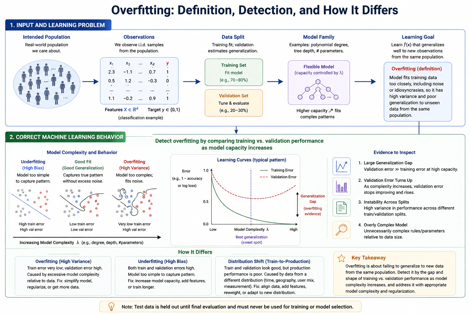
Overfitting is a failure to generalize. The model learns the training records so closely that it also captures noise or sample-specific details that do not repeat reliably in new observations. Training error can therefore become very low while validation error on unseen observations from the same intended population remains much higher. The main evidence is the training-validation gap. I would also inspect what happens as model complexity increases and whether performance is unstable across different validation splits. These checks help separate overfitting from underfitting and from a genuine train-to-production distribution shift.

Useful Questions to Ask the Interviewer
  1. Are the training and validation observations sampled from the same intended population?
  2. Are we comparing the same evaluation measure on the training and validation sets?
  3. Is there a separate held-out test set used only after model selection?
  4. Do we have results from multiple validation splits or cross-validation folds?
  5. If production performance is worse, is there evidence that the production data distribution changed?
What is overfitting, and how would you detect it? diagram
How to Explain It in an Interview

The learning goal is not just to fit records the model has already seen. The goal is to learn a function that performs well on new observations from the same intended population. Overfitting occurs when the model becomes too adapted to the particular training sample, including noise or idiosyncrasies that do not generalize.

I would first compare training and validation evidence. The model is fitted on the training set. Validation data remains separate from model fitting and is used during model selection to estimate generalization. I would compare the same evaluation measure on both sets. A large generalization gap, such as very low training error but much higher validation error, is classic evidence of overfitting.

I would also inspect performance as model capacity increases. Greater capacity can come from choices such as a higher polynomial degree, a deeper tree, or more model parameters. Training error usually keeps decreasing as capacity increases. Validation error may decrease at first as the model captures useful structure, then stop improving and begin to rise once the model starts fitting training-specific noise. The complexity where validation performance is best is a better choice than simply selecting the model with the lowest training error.

Another useful signal is instability across data splits. A high-variance model can produce noticeably different validation performance when the training and validation samples change. That suggests the learned behavior depends too strongly on the particular training sample rather than on stable structure in the intended population.

Underfitting has a different pattern. An underfit model is too simple to capture the important pattern, so both training and validation errors are high. With overfitting, training error is typically very low while validation error is substantially higher.

A genuine train-to-production distribution shift is also different. If training and same-population validation performance are both good but production performance becomes poor, I would investigate whether the production population, feature distribution, measurement process, geography, user mix, or other data-generating conditions changed. That pattern points toward distribution shift rather than ordinary overfitting.

If overfitting is present, I would select model complexity using validation evidence rather than training fit alone. Depending on the model family, I might simplify the model, add appropriate regularization, or obtain more representative training data. I would then re-evaluate using validation data. A separate test set should stay untouched throughout training and model selection and be used only for the final evaluation.

Technical Approach
  1. Split the available same-population data so model fitting uses only the training set and model-selection evidence comes from validation data.
  2. Fit the candidate model on the training set.
  3. Measure performance on both the training and validation sets using the same evaluation measure.
  4. Compare the results and inspect the generalization gap.
  5. Examine performance as model capacity changes. Watch for training error continuing to fall while validation error stops improving or rises.
  6. Check stability across different validation splits or cross-validation folds when appropriate.
  7. If both training and validation errors are high, diagnose underfitting rather than overfitting.
  8. If training and same-population validation are good but production performance is poor, investigate distribution shift rather than assuming overfitting.
  9. Choose model complexity and regularization using validation evidence.
  10. Keep the held-out test set untouched until the final evaluation.
Practical Insights

A more flexible model can capture useful patterns, but it can also fit random details in the training sample. This creates a variance tradeoff: training performance may keep improving while performance on new data becomes worse. A simpler or more regularized model may fit the training set slightly less well but generalize better. Cross-validation gives better evidence about stability because it repeats the evaluation across different splits, but it requires fitting the model multiple times. More representative training data can also help, but collecting and maintaining additional data has cost.

Why Interviewers Ask This

This question tests whether the candidate understands generalization, bias and variance, model capacity, and the role of validation data. It also tests whether the candidate can distinguish a model that fits training-specific noise from a model that is too simple, and from a model whose production data no longer follows the distribution represented by the training and validation data.

Common interview mistakes

Common mistakes are calling any validation error overfitting without comparing it with training performance; assuming lower training error always means a better model; confusing underfitting with overfitting even though underfitting normally has poor training performance too; treating one noisy validation result as definitive evidence instead of considering stability across splits; blaming overfitting when training and validation are good but production data has shifted; and using the held-out test set repeatedly for model selection.

Interview tip

Present the answer in a simple order: define overfitting as poor generalization, explain the training-validation gap, mention validation error rising with excessive model complexity, contrast it with underfitting, then explain that good validation but poor production performance suggests distribution shift. Finish by noting that the test set stays untouched until final evaluation.

Interviewer may ask next
What if training and validation performance are both poor?

That pattern is more consistent with underfitting than overfitting. The model is not fitting even the training data well, so it may be too simple to capture the important pattern. I would investigate model capacity and the learning setup before adding stronger regularization. After changing the model appropriately, I would compare training and validation performance again and check whether both improve without creating a large generalization gap.

What if training and validation performance are both good, but production performance becomes much worse?

That pattern does not look like ordinary overfitting if the validation data was representative of the intended population and remained separate from training. I would investigate train-to-production distribution shift. I would compare relevant feature distributions and, when observable, target distributions across training, validation, and production data, and check whether the population, measurement process, geography, user mix, or other data-generating conditions changed. If the production distribution changed, the response may require better-aligned data, new features, reweighting, retraining, or adaptation to the new distribution rather than simply reducing model complexity.

5. Explain the bias-variance trade-off.Machine LearningEasy

Question Details

Describe bias and variance as sources of prediction error for a model trained on repeated samples from the same population. Explain how model flexibility, training-set size, noise, and regularization affect the trade-off, and connect it to the pattern you would expect in training and validation performance.

Short Interview Answer (30-60 seconds)

Bias is systematic error from a model that is too simple, while variance is sensitivity to the particular training sample. More flexibility usually lowers bias but raises variance. We want the balance that minimizes validation error. More data usually reduces variance, while regularization reduces effective flexibility and can trade lower variance for higher bias.

Detailed Explanation

The bias-variance trade-off explains why increasing model flexibility does not always improve predictions on new data. Imagine repeatedly drawing training sets from the same population and fitting the same learning procedure each time. Bias measures systematic error in the average fitted prediction relative to the true pattern. Variance measures how much fitted predictions change across those training sets. Simple models often have high bias and low variance. Flexible models often have lower bias but higher variance. The goal is good generalization: low prediction error on unseen data, not simply the lowest training error.

Useful Questions to Ask the Interviewer
  1. Should I explain the trade-off using squared-error prediction and the bias-variance decomposition?
  2. Would you like me to connect the theory to training and validation error as model flexibility changes?
  3. Should I also discuss how training-set size, noise, and regularization affect the trade-off?
Explain the bias-variance trade-off. diagram
How to Explain It in an Interview

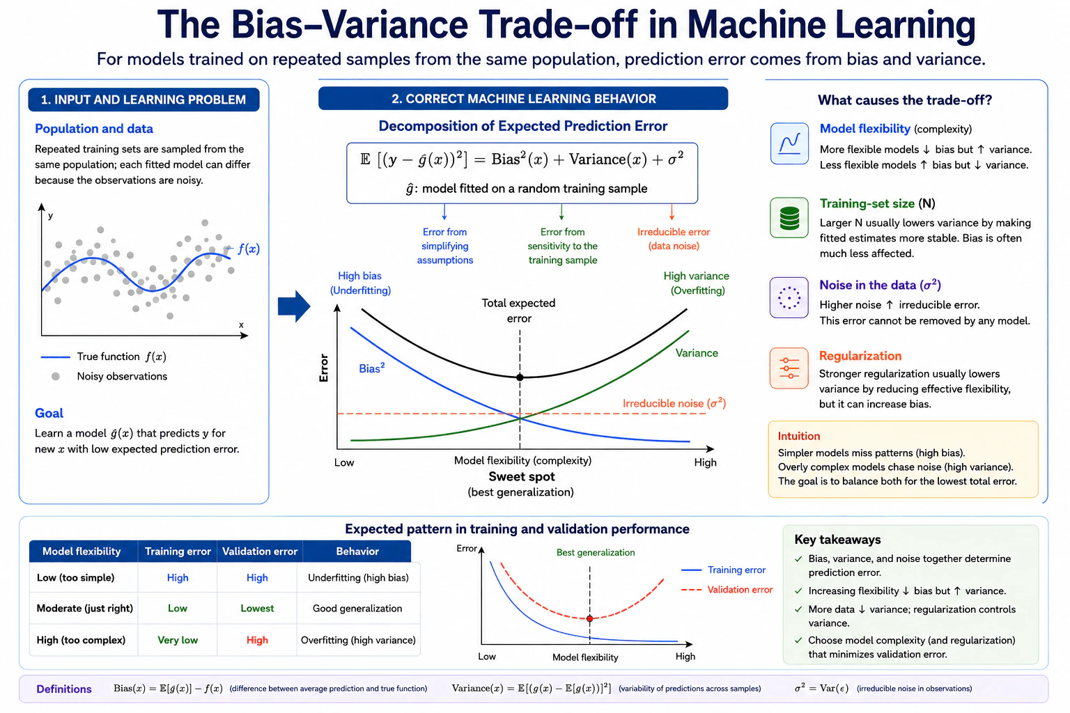
Start with repeated training samples from the same population. Because the observations contain noise, fitting the same learning procedure to different samples can produce different fitted predictors, written as ĝ(x).

For squared-error prediction, the expected prediction error can be summarized as:

E[(y − ĝ(x))²] = Bias²(x) + Variance(x) + σ²

Here, Bias(x) = E[ĝ(x)] − f(x). It measures the difference between the average fitted prediction and the true function f(x). Variance(x) = E[(ĝ(x) − E[ĝ(x)])²]. It measures how much predictions vary across repeated training samples. The term σ² represents irreducible noise in the observations. No fitted model can completely remove that noise.

Now connect this to model flexibility. A very simple model may miss real structure in the population. Its predictions stay relatively similar across training samples, so variance is low, but its systematic error can be large. This is high bias and underfitting. As flexibility increases, the model can represent more of the true pattern, so bias usually decreases.

If flexibility becomes too high, the fitted model can react strongly to the particular observations and noise in one training sample. Different training samples can then produce noticeably different fitted models. Variance becomes high. This is the overfitting region.

The useful operating point is between these extremes. In the diagram, bias squared decreases as flexibility increases, variance increases, and irreducible noise stays as an error floor. Their combination produces a U-shaped total expected error curve, with the best generalization near its minimum.

Training and validation performance show the same idea from another angle. Training error generally keeps decreasing as flexibility increases because a flexible model can fit the training observations more closely. Validation error usually decreases at first because the model removes underfitting. After a certain point, validation error rises because extra flexibility begins fitting sample-specific noise. Among the models being compared, the model near the minimum validation error gives the best generalization.

Training-set size mainly affects variance. With a larger training set drawn from the same population, fitted estimates are usually more stable, so variance decreases. Bias is often much less affected because it mainly comes from the assumptions and effective flexibility of the learning procedure.

Noise changes the minimum achievable prediction error. Higher observation noise increases the irreducible error term σ². Increasing model flexibility cannot eliminate that noise. A very flexible model may instead chase the noise, increasing variance.

Regularization controls effective flexibility. Stronger regularization usually constrains the fitted model, which can reduce variance. The trade-off is that too much regularization can increase bias and cause underfitting. In practice, model complexity and regularization are chosen using validation performance rather than training error alone.

A concise summary is: too simple means high bias and underfitting; too flexible means high variance and overfitting; more data usually reduces variance; noise creates an irreducible error floor; and stronger regularization usually lowers effective flexibility. The goal is the balance that minimizes validation error and gives the strongest generalization.

Technical Approach
  1. Start with repeated training sets sampled from the same population.
  2. Define bias as systematic error in the average fitted prediction.
  3. Define variance as sensitivity of the fitted prediction to the particular training sample.
  4. Explain that increasing flexibility usually decreases bias and increases variance.
  5. Identify underfitting at the high-bias end and overfitting at the high-variance end.
  6. Connect this to training error generally decreasing while validation error typically reaches a minimum and then rises.
  7. Explain that larger training sets usually reduce variance, higher noise raises irreducible error, and stronger regularization usually lowers variance while potentially increasing bias.
  8. Choose model flexibility and regularization near the minimum validation error.
Practical Insights

A simpler model is usually more stable across different training samples, but it may miss the real pattern. A more flexible model can capture richer patterns, but it can become sensitive to noise and to the particular sample it saw. More training data usually makes fitted estimates more stable and lowers variance. Stronger regularization also reduces effective flexibility, but too much can create underfitting. Higher data noise raises an error floor that no model can completely remove. The practical trade-off is choosing enough flexibility to learn the signal without fitting sample-specific noise.

Why Interviewers Ask This

Interviewers want to see whether you understand why a model can fail either by being too simple or by reacting too strongly to the particular training sample it receives. They also want you to connect bias and variance to model flexibility, training-set size, noise, regularization, underfitting, overfitting, and the different patterns seen in training and validation performance.

Common interview mistakes

Common mistakes are saying bias means training error, saying variance is the same as observation noise, assuming more flexible models are always better, or claiming regularization always improves performance. Another mistake is choosing the model with the lowest training error instead of considering validation performance. It is also incorrect to say that more training data removes irreducible noise. More data usually reduces estimation variance, while σ² remains part of the prediction-error floor.

Interview tip

Explain the trade-off as one connected story: repeated training samples create bias and variance effects; flexibility moves the model from underfitting toward overfitting; training error keeps falling while validation error reaches a useful minimum; then explain how more data, noise, and regularization change that picture.

Interviewer may ask next
If you collect a much larger training set from the same population, which part of the bias-variance trade-off changes most?

Variance usually decreases the most because the fitted model is based on more observations and becomes less sensitive to which particular sample was drawn. Bias is often much less affected because it mainly reflects the assumptions and effective flexibility of the learning procedure. Irreducible noise does not disappear simply because the training set becomes larger.

What happens if you make regularization much stronger in a model that is currently overfitting?

Stronger regularization reduces the model's effective flexibility, so variance usually decreases and validation performance may improve. However, continuing to strengthen regularization can eventually make the model too constrained. Bias then increases, the model begins to underfit, and validation error can rise again. The useful regularization level is therefore chosen around the best validation performance rather than by maximizing regularization.

6. When would you use L1 regularization instead of L2 regularization?Machine LearningEasy

Question Details

Compare L1 and L2 penalties for a supervised model whose features may be correlated and measured on different scales. Address their effects on coefficient shrinkage, sparsity, stability, feature selection, and optimization, and state what preprocessing or validation is needed before choosing between them.

Short Interview Answer (30-60 seconds)

I would prefer L1 when I want a sparse, interpretable model or automatic feature selection because it can drive some coefficients exactly to zero. I would prefer L2 when I want to retain predictors and get more stable coefficients, especially with correlated features. I would standardize features first and choose the penalty and its strength using validation or cross-validation.

Detailed Explanation

L1 and L2 regularization both control model complexity by penalizing large coefficients, but they behave differently. L1 uses the sum of absolute coefficient values, so it can force some coefficients exactly to zero and create a sparse model. L2 uses the sum of squared coefficients, so it usually shrinks every coefficient toward zero without removing predictors. This matters when features are correlated or measured on different scales. Before comparing them, standardize features, avoid preprocessing leakage, and tune the regularization strength using validation or cross-validation rather than choosing it from the training fit alone.

Useful Questions to Ask the Interviewer
  1. Is the main goal predictive performance, model interpretability, or selecting a smaller set of features?
  2. Are the predictors strongly correlated with one another?
  3. Are the features measured on very different scales or units?
  4. Do we expect only a small subset of predictors to be useful, or many predictors to have small effects?
  5. What validation procedure and evaluation metric should be used to compare the regularized models?
When would you use L1 regularization instead of L2 regularization? diagram
How to Explain It in an Interview

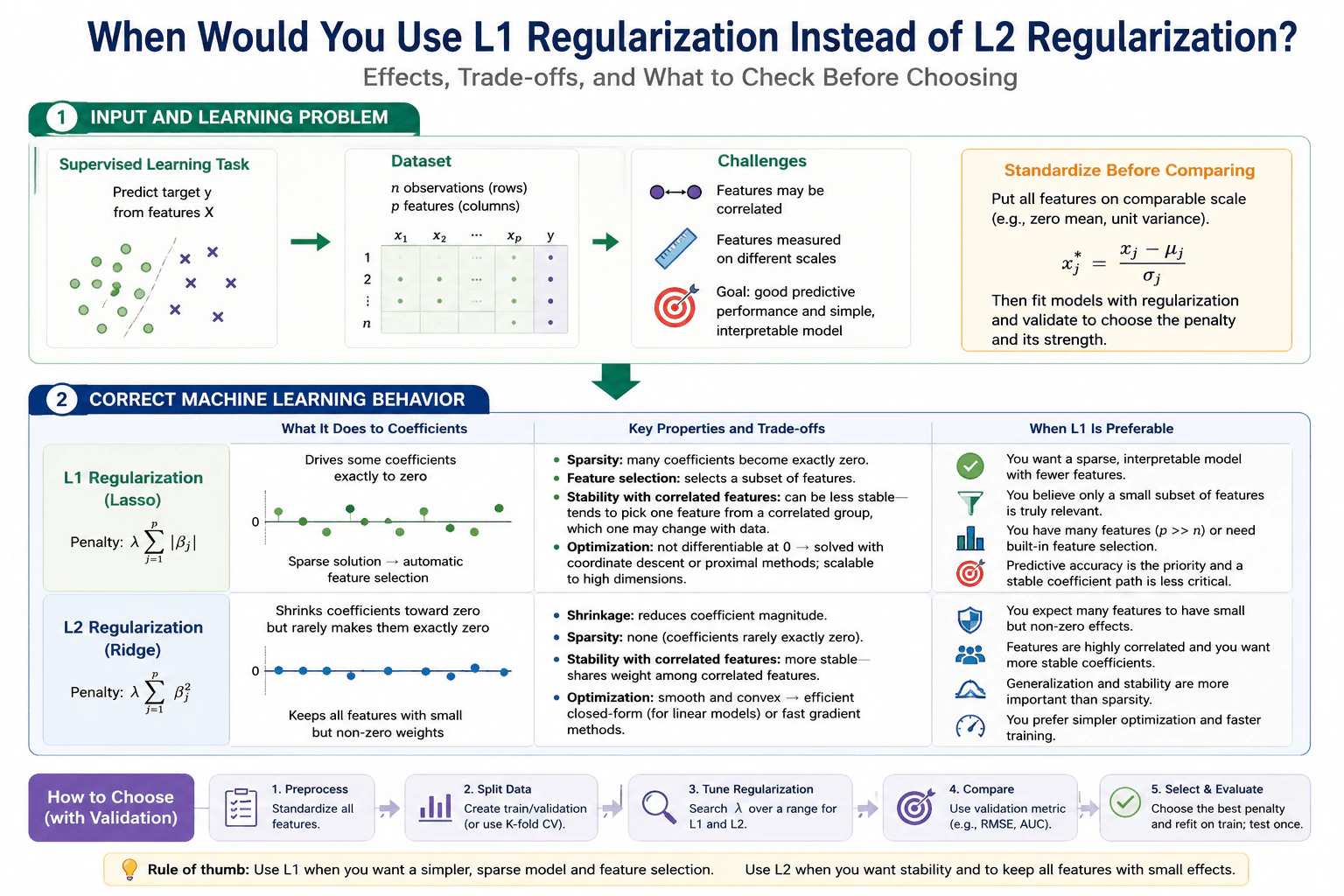
Start with the penalties. For coefficient vector β and regularization strength λ, L1 adds a penalty proportional to λΣ|β_j|. L2 adds a penalty proportional to λΣβ_j². The regularization strength λ is a hyperparameter: larger values apply stronger shrinkage.

The main reason to choose L1 is sparsity. L1 can drive some coefficients exactly to zero. Those predictors effectively disappear from the fitted model, so L1 performs embedded feature selection. This is useful when you believe only a small subset of the available features is truly useful, when there are many irrelevant or noisy predictors, when the number of features is large relative to the number of observations, or when a simpler and more interpretable model is valuable.

L2 behaves differently. It shrinks coefficients toward zero but rarely makes them exactly zero. It therefore tends to retain predictors with smaller weights. This can be preferable when many features may each contribute a small amount of useful signal and you do not want the regularizer to remove them.

Correlated predictors are an important tradeoff. With a group of strongly correlated features, L1 can be less stable because it may select one feature from the group and set others to zero. Which feature is selected can change when the data changes slightly. L2 is usually more stable in this situation because it can distribute coefficient weight across correlated predictors instead of selecting only one representative.

The optimization behavior is also different. The L1 penalty is not differentiable at zero, so algorithms commonly use methods such as coordinate descent or proximal optimization. L2 is smooth and differentiable. For linear ridge regression, a closed-form solution exists, and gradient-based optimization is also straightforward.

Feature scale must be handled before comparing L1 and L2. Because both penalties act directly on coefficient magnitudes, predictors measured on very different scales can receive unfairly different effective penalties. Standardize the features, for example to zero mean and unit variance. Any learned preprocessing must be fitted only on the training portion within each validation fold so information from validation or test data does not leak into training.

Then compare the penalties fairly. Split the data so the final test set remains held out. Tune λ over an appropriate range for both L1 and L2 using validation data or K-fold cross-validation. Use the same folds and an evaluation metric appropriate to the supervised task. If predictive performance is the main priority, neither penalty should be chosen by rule of thumb alone: select the one that performs better under the same validation protocol, while also considering whether coefficient stability or sparsity matters.

After choosing the penalty and λ from validation performance and the desired interpretability-versus-stability tradeoff, refit the selected model on the allowed training data and evaluate it once on the held-out test set.

The decision is therefore not that L1 is universally better than L2. Prefer L1 when sparsity, automatic feature selection, and a simpler model are important and some instability among correlated predictors is acceptable. Prefer L2 when retaining predictors, stable coefficients, and sharing weight across correlated features are more important.

Technical Approach
  1. Identify the goal: decide whether sparsity and feature selection or coefficient stability and retention of predictors matter more.
  2. Inspect the feature setup, especially different measurement scales and strong correlations among predictors.
  3. Split the data so validation is used for model selection and the final test set remains untouched.
  4. Fit preprocessing only on the training data. Standardize numeric features to comparable scales before applying either penalty.
  5. Fit L1-regularized and L2-regularized versions of the same supervised model under the same validation procedure.
  6. Tune the regularization strength λ for each model using validation data or K-fold cross-validation and the same task-appropriate metric.
  7. Compare validation performance together with model properties: number of zero coefficients, interpretability, and coefficient stability when predictors are correlated.
  8. Prefer L1 when a sparse model and embedded feature selection are valuable and its lower stability with correlated predictors is acceptable. Prefer L2 when keeping predictors and obtaining more stable shrinkage is more important.
  9. If predictive performance is the main priority, let the validation result decide between L1 and L2 rather than assuming one penalty is always better.
  10. Refit the selected configuration on the allowed training data and evaluate it once on the held-out test set.
Practical Insights

Statistically, L1 can reduce a model to fewer active features, which can make the model easier to explain, but its selected features can be unstable when predictors are strongly correlated. L2 usually keeps predictors and spreads weight more smoothly across correlated features, so coefficients are often more stable. Computationally, L1 is harder to optimize because its penalty has a sharp point at zero, so specialized methods such as coordinate descent or proximal methods are common. L2 is smooth and easier to optimize, and linear ridge regression even has a closed-form solution. Both approaches add model-selection cost because λ should be tuned with validation or cross-validation. Standardization and leakage-safe preprocessing are also required for a fair comparison when features use different scales.

Why Interviewers Ask This

This question tests whether you understand how L1 and L2 penalties change model coefficients and whether you can connect those mathematical differences to practical model selection. A strong answer should explain sparsity, feature selection, correlated-feature stability, scale sensitivity, optimization, regularization-strength tuning, and correct validation rather than simply saying that L1 creates zeros and L2 does not.

Common interview mistakes

Common mistakes are saying that L1 is always better because it performs feature selection, or that L2 cannot reduce overfitting. Another mistake is forgetting that L1 may select one feature somewhat arbitrarily from a correlated group, making the selected set less stable. Candidates also sometimes claim that L2 sets coefficients exactly to zero; normally it only shrinks them toward zero. A major practical mistake is comparing penalties without standardizing differently scaled features. Another is fitting the scaler before the train-validation split, which causes preprocessing leakage. Finally, λ should not be chosen from training performance alone; it should be tuned using validation or cross-validation while keeping the final test set held out.

Interview tip

Lead with the decision rule: L1 for sparsity and feature selection, L2 for stable shrinkage and retaining predictors. Then immediately mention the correlated-feature tradeoff, standardization, and cross-validation for λ. If prediction quality is the priority, say that validation should decide between the penalties.

Interviewer may ask next
What happens if several predictors are strongly correlated and you use L1 regularization?

L1 may keep one predictor from the correlated group and drive the coefficients of others to zero. Because those predictors contain similar information, a small change in the training data can cause a different member of the group to be selected. That makes the selected feature set and individual coefficients less stable. If stable coefficients across correlated predictors are more important than sparsity, L2 is usually a better choice because it can retain the correlated predictors and distribute weight across them.

How would your choice change if prediction stability became more important than having a sparse, easily interpreted model?

I would lean toward L2, especially when predictors are correlated or many features are expected to have small but real effects. L2 shrinks coefficients smoothly without normally setting them to zero and tends to spread weight across correlated predictors, which generally gives more stable coefficients. I would still standardize features and tune λ using the same validation procedure, because the final choice should be supported by validation performance rather than by the penalty type alone.

7. How do gradient boosting and random forests differ?Machine LearningMedium

Question Details

Compare the two tree-ensemble methods for the same supervised tabular task. Cover how trees are trained and combined, how each method responds to bias, variance, noisy labels, correlated features, class imbalance, and hyperparameters, and how you would choose between them under accuracy, latency, interpretability, and retraining constraints.

Short Interview Answer (30-60 seconds)

Random forests train many trees independently on bootstrapped data and average or vote, mainly reducing variance. Gradient boosting trains trees sequentially to correct previous errors, often reducing bias and improving accuracy. Random forests are usually simpler and more robust; boosting usually needs more tuning and regularization.

Detailed Explanation

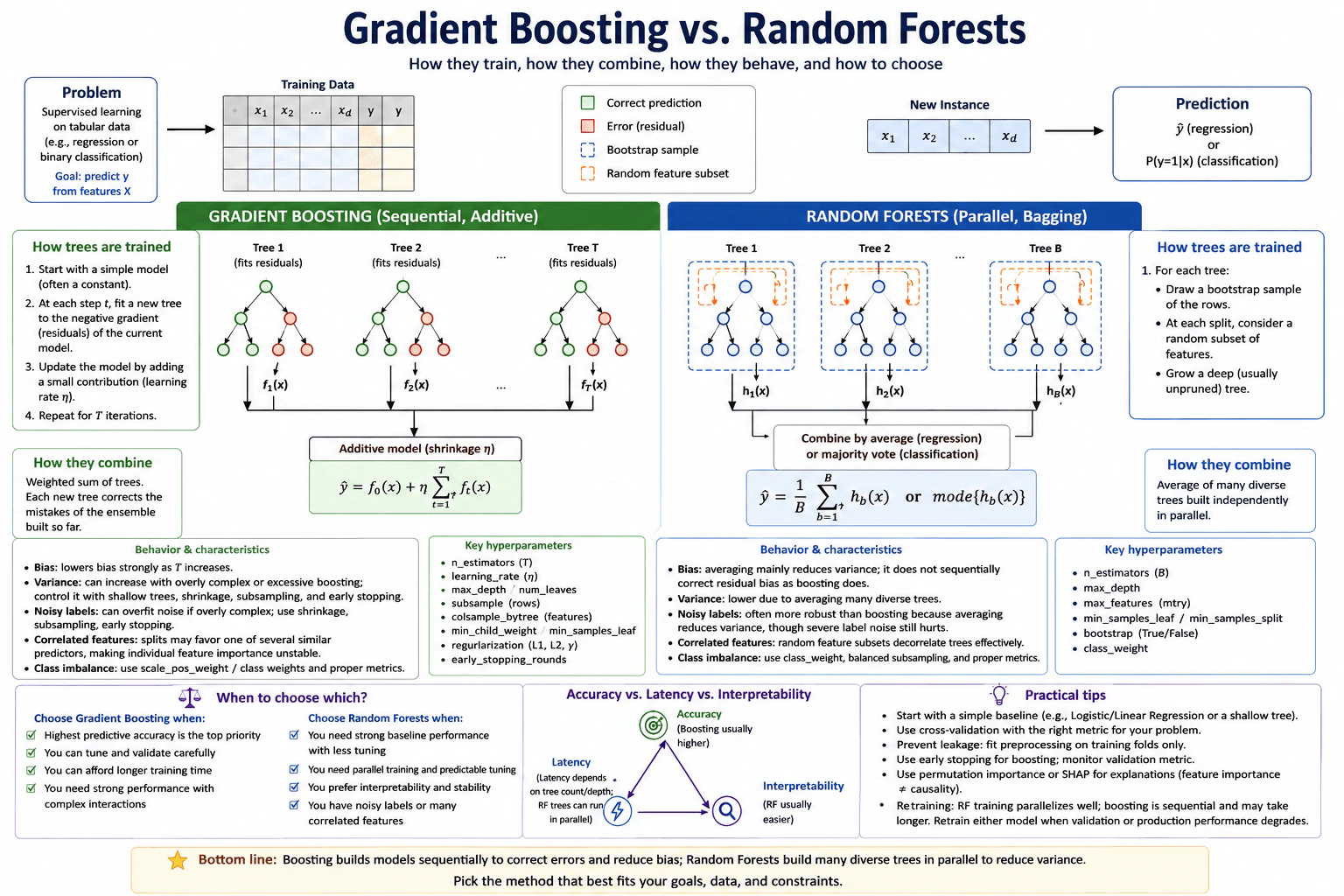
Both methods are supervised tree ensembles for tabular prediction, but they create diversity in different ways. A random forest trains many trees independently on bootstrap samples and random feature subsets, then combines their outputs by averaging for regression or majority voting for classification. Gradient boosting builds trees sequentially. Each new tree fits the residual error, or more generally the negative gradient of the current loss, and is added with a learning rate. This difference drives their behavior: forests mainly reduce variance, while boosting can reduce bias more aggressively but can overfit without careful control.

Useful Questions to Ask the Interviewer
  1. Is the main goal maximum predictive accuracy, or are training time, inference latency, stability, and interpretability equally important?
  2. How noisy are the labels, and do we expect many correlated features?
  3. Is the target highly imbalanced, and what evaluation metric reflects the real error cost?
  4. How often must the model be retrained, and how much training time is available?
  5. Are prediction latency or model-explanation requirements strict in production?
How do gradient boosting and random forests differ? diagram
How to Explain It in an Interview

Start with a simple relevant baseline and evaluate both methods with the same leakage-safe validation procedure and a metric that matches the decision cost. Fit any learned preprocessing only on the training folds.

1. How random forests train

For each tree, draw a bootstrap sample of the training rows. At each split, consider only a random subset of features. The trees are trained independently and can therefore be parallelized. Individual trees can have high variance, but averaging many diverse trees reduces that variance. For regression, average the tree predictions. For classification, combine the tree predictions by majority vote.

2. How gradient boosting trains

Gradient boosting starts with a simple initial prediction. It then adds trees one at a time. Each new tree is trained to improve the current ensemble by fitting residuals or, more generally, the negative gradient of the chosen loss. The ensemble is additive: the initial prediction plus the learning-rate-scaled contributions of the trees. A small learning rate, shallow trees, subsampling, regularization, and early stopping can control overfitting.

3. Bias and variance

Random forests mainly attack variance. Bootstrap sampling and random feature subsets make the trees more diverse, so averaging becomes more effective. Averaging does not sequentially correct residual bias in the way boosting does.

Gradient boosting can reduce bias strongly because every new tree focuses on errors left by the current ensemble. However, variance can rise if the trees become too complex or boosting continues for too many iterations. Shallow trees, shrinkage, subsampling, and early stopping are important controls.

4. Noisy labels

Random forests are often more robust to noisy labels than boosting because averaging many diverse trees reduces variance. Severe label noise still hurts performance.

Boosting can chase noisy examples because later trees repeatedly focus on observations that the current model predicts poorly. With noisy data, use smaller learning rates, limited tree complexity, subsampling, regularization, and early stopping.

5. Correlated features

Random forests use random feature subsets at splits, which helps decorrelate trees. With strongly correlated predictors, model importance can still be distributed across related features.

In gradient boosting, splits may favor one of several similar predictors. That can make the importance assigned to any single correlated feature unstable. Feature importance should not be interpreted as causality. Permutation importance or SHAP can help explain model behavior, but correlated features still require careful interpretation.

6. Class imbalance

Neither method automatically solves class imbalance. For random forests, useful controls include class weights, balanced sampling, and an evaluation metric appropriate for the decision. For gradient boosting, class weights, positive-class weighting when supported, custom losses when appropriate, and threshold tuning can help. The validation metric and decision threshold should reflect the real cost of false positives and false negatives rather than relying only on overall accuracy.

7. Important hyperparameters

For a random forest, important hyperparameters include the number of trees, maximum depth, number of features considered at each split, minimum samples required for splits or leaves, and whether bootstrap sampling is used.

For gradient boosting, important hyperparameters include the number of boosting iterations, learning rate, tree depth or number of leaves, row subsampling, feature subsampling, minimum leaf constraints, regularization, and early stopping. The learning rate and number of trees interact strongly: a smaller learning rate usually requires more boosting iterations.

8. Accuracy

If maximum predictive accuracy is the priority and careful validation and tuning are available, gradient boosting is often a strong choice for tabular data. Its sequential error correction can capture complex patterns efficiently. That is not a guarantee, so both methods should be compared with the same validation procedure.

Random forests provide a strong baseline and can perform very well with less tuning. Their stability is especially useful when labels are noisy or when fast experimentation matters.

9. Latency and training

Random-forest trees are independent, so training can be parallelized. Inference latency still depends on the number and depth of trees, although independent tree evaluations can also be parallelized in some systems.

Gradient boosting is sequential during training because tree t depends on the ensemble created by earlier trees. This can make retraining slower. Inference latency for either method depends on the final number and complexity of the trees, so it should be measured rather than assumed.

10. Interpretability

Both ensembles are harder to interpret than a single shallow tree. A random forest is often somewhat easier to reason about operationally because it averages independently trained trees, while gradient boosting has a sequential additive structure. For either model, use tools such as permutation importance or SHAP when explanations are required, and remember that feature importance describes model behavior rather than causality.

11. Retraining constraints

If retraining must be frequent or training resources are constrained, random forests are attractive because independent trees parallelize naturally and tuning is often less sensitive. Gradient boosting may take longer because training is sequential and often depends on careful early stopping and hyperparameter selection. For either model, retrain when validation or production performance degrades rather than assuming a fixed schedule is always correct.

12. Final choice

Choose gradient boosting when predictive accuracy is the main priority, you can tune and validate carefully, longer sequential training is acceptable, and complex feature interactions matter. Choose a random forest when you want a strong baseline, stable behavior with less tuning, parallel training, and greater robustness to noisy labels. For both, handle class imbalance correctly, prevent leakage, use the right validation metric, and verify performance under the actual latency and retraining constraints.

Technical Approach
  1. Start with a simple relevant baseline before adding ensemble complexity.
  2. Create one leakage-safe validation procedure and use the same folds for both models.
  3. Choose an evaluation metric that matches the real prediction error cost, especially when classes are imbalanced.
  4. Train a random forest using bootstrap samples and random feature subsets; tune tree count, depth, feature subset size, and leaf constraints.
  5. Train gradient boosting sequentially; tune learning rate, tree complexity, number of iterations, subsampling, regularization, and early stopping.
  6. Compare validation performance, stability, behavior on noisy or imbalanced data, and important error slices.
  7. Measure training time and inference latency under the intended operational constraints instead of assuming one method is always faster.
  8. Compare explanation quality using an appropriate interpretation method such as permutation importance or SHAP, without treating feature importance as causal.
  9. Choose the model that gives the best overall tradeoff among predictive performance, robustness, latency, interpretability, and retraining cost.
Practical Insights

Random forests can train many trees at the same time because the trees are independent. More or deeper trees increase memory use and prediction work, but forests are usually straightforward to tune and stable. Gradient boosting must build trees in sequence, so training is harder to parallelize. It can reach strong accuracy with shallow trees, but the learning rate, number of trees, depth, subsampling, and regularization interact. Too much boosting can overfit. Prediction cost for both methods grows with the number and depth of trees. Random forests often use many trees, while boosting may need careful tuning and early stopping. Retraining a forest can be operationally simpler because independent trees parallelize well; boosting may take longer because each new tree depends on the current ensemble.

Why Interviewers Ask This

This question tests whether a candidate understands two major tree-ensemble strategies and can connect their training mechanics to bias, variance, noisy labels, correlated features, class imbalance, hyperparameters, accuracy, latency, interpretability, and retraining constraints. A strong answer explains why bagging and random feature selection make random forests stable, why sequential residual correction makes gradient boosting powerful but easier to overfit, and how those differences affect a practical model-selection decision.

Common interview mistakes

Common mistakes are saying random forests reduce both bias and variance equally, saying boosting simply trains trees on wrongly classified rows, or forgetting that boosting follows residuals or the negative gradient of a loss. Another mistake is claiming that random forests are always faster at inference; latency depends on tree count, depth, implementation, and available parallelism. Candidates also often ignore noisy labels, correlated features, class imbalance, and the interaction between learning rate and number of boosting rounds. Finally, do not claim feature importance proves causality or that better offline accuracy guarantees better production performance.

Interview tip

Lead with the central contrast: random forests build diverse trees independently and average or vote to reduce variance; gradient boosting builds trees sequentially to correct errors and reduce bias. Then connect that difference to noise, tuning, accuracy, latency, interpretability, and retraining. Finish with a conditional model-selection recommendation rather than declaring one method universally better.

Interviewer may ask next
What changes if the training labels are noisy?

I would usually expect the random forest to be more forgiving because averaging many diverse trees reduces variance. Gradient boosting deserves more caution because later trees repeatedly focus on errors left by earlier trees, so mislabeled observations can attract repeated attention. For boosting, I would reduce tree complexity, use a smaller learning rate, consider row subsampling and regularization, and use early stopping on validation data. I would still compare both models with the same leakage-safe validation procedure because severe label noise can hurt either method.

What if retraining must happen frequently and prediction latency is also strict?

I would measure both constraints directly. Random-forest training is attractive because the trees are independent and can be trained in parallel, which can make frequent retraining simpler. Gradient boosting is sequential during training, so each tree depends on the current ensemble and retraining may take longer. For inference, I would not assume the forest is automatically faster: latency depends on the number and depth of trees for both methods and on whether parallel evaluation is available. If both satisfy the latency budget, I would then choose using validation quality, stability, interpretability needs, and retraining cost.

8. How would you train a classifier on a highly imbalanced target?Machine LearningMedium

Question Details

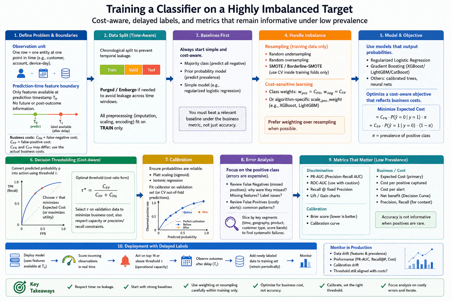
Assume the positive class is rare, false negatives and false positives have different business costs, and labels are available only after a delay. Define the observation unit and prediction-time feature boundary, then discuss split strategy, baselines, resampling or weighting, objective choice, thresholding, calibration, error analysis, and metrics that remain informative under low prevalence.

Short Interview Answer (30-60 seconds)

I would define the observation and prediction-time feature boundary first, then use a chronological split and training-only preprocessing. I would start with simple baselines, prefer class weighting or use training-only resampling, train a probabilistic classifier, calibrate it if needed, and choose the threshold on validation data from business costs and capacity constraints. I would focus on PR-AUC, precision, recall, calibration, expected cost, and delayed-label monitoring rather than accuracy.

Detailed Explanation

A highly imbalanced classifier should be designed around the decision and its business cost, not around raw accuracy. One observation is one entity at one prediction time. The target is a later binary outcome, and the model may use only information available at or before that prediction timestamp. Because the positive class is rare and labels arrive after a delay, the newest observations may not yet have mature labels. I would therefore use leakage-safe time splits, establish strong baselines, handle imbalance only inside training, produce reliable probability estimates, choose a cost-aware operating threshold, and evaluate both low-prevalence metrics and realized business cost.

Useful Questions to Ask the Interviewer
  1. What exactly is one observation, and at what timestamp must the prediction be made?
  2. How is the positive target defined, and how long after prediction does the label become available?
  3. Which features are guaranteed to be available at prediction time?
  4. What are the business costs of a false negative and a false positive?
  5. Is there an operational limit on how many positive predictions can be reviewed or acted on?
  6. Do we need well-calibrated probabilities, or is ranking plus a decision threshold sufficient?
How would you train a classifier on a highly imbalanced target? diagram
How to Explain It in an Interview

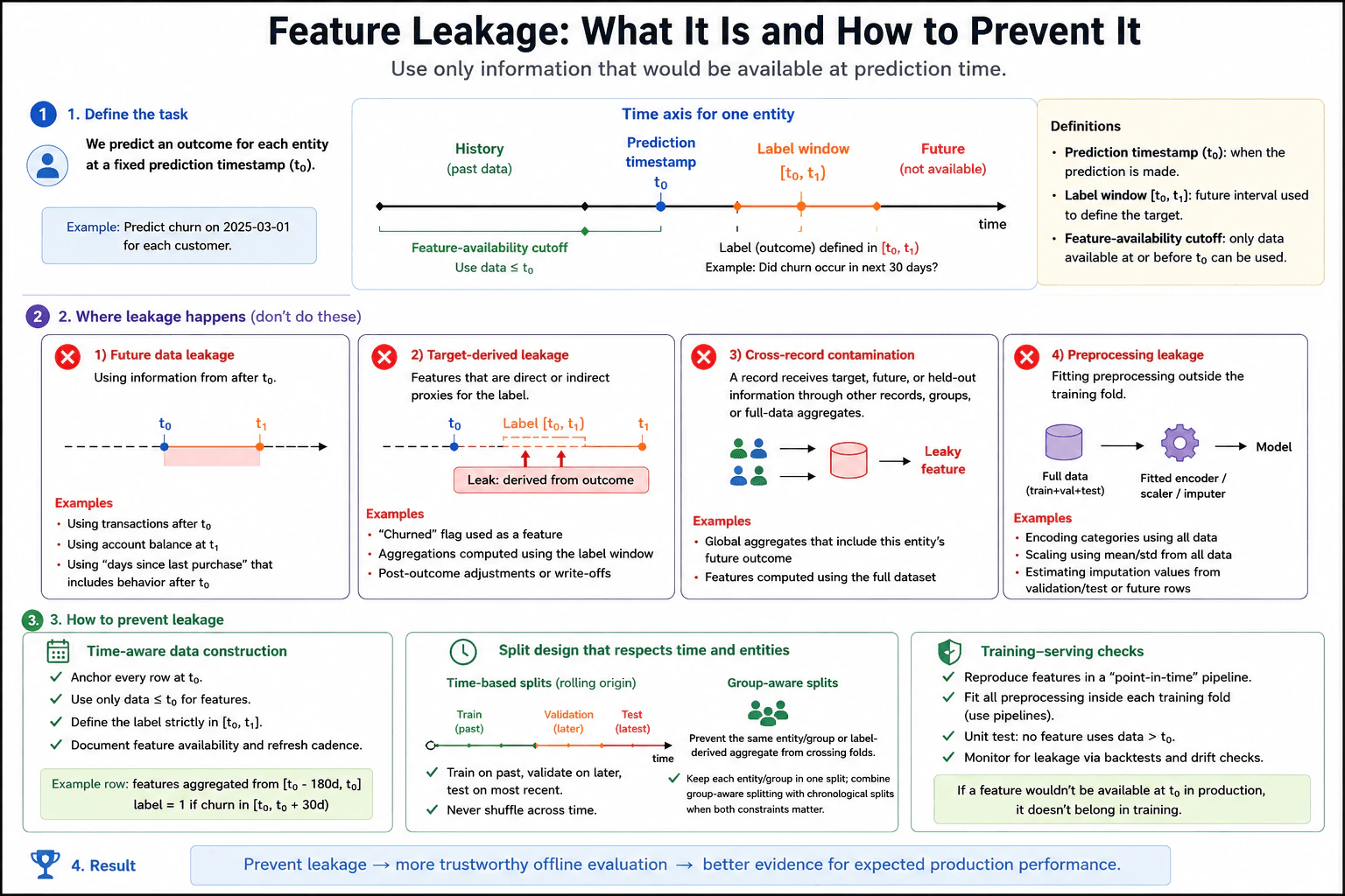
First, define the observation and feature boundary. One row represents one entity at one prediction timestamp. Only features known at or before that timestamp can be used. Future events, post-outcome information, and features derived from the final label are excluded. This prevents target leakage and temporal leakage.

Next, split the data in time order. Use an earlier period for training, a later period for validation, and a still later labeled period for final testing. If repeated observations from the same entity could make evaluation unrealistically easy, also prevent entity leakage across splits. A purge or embargo around neighboring time windows can be useful when adjacent examples share information that would otherwise leak across the boundary. Learned preprocessing such as imputation, scaling, encoding, feature selection, and resampling must be fit only on the allowed training data.

Then build baselines before adding complexity. An all-negative classifier is a useful warning baseline because it can achieve apparently high accuracy while recalling zero positives. A prior-probability baseline and a simple regularized logistic-regression model provide stronger comparisons. A complex model should beat a relevant baseline on the metric or business objective that matters, not merely on accuracy.

For the imbalance itself, I would usually try class or sample weighting first because it keeps the original training examples and is operationally simple. Positive and negative errors can receive different weights based on their business importance. Some algorithms also expose imbalance-specific weighting parameters. If weighting is not enough, random oversampling, random undersampling, or methods such as SMOTE can be considered, but resampling must occur only within each training fold. Validation and test examples must never participate in generating synthetic or duplicated training samples.

The model should produce a score that can be calibrated into a useful probability when probability estimates matter. Suitable model families include regularized logistic regression, gradient-boosted trees such as XGBoost, LightGBM, or CatBoost, calibrated tree models, and neural networks when the problem justifies them. The loss can be cost-sensitive or class-weighted. Focal loss is another option when hard minority examples deserve additional emphasis. Regularization and hyperparameters should be tuned using only the training and validation process, not the final test set.

Calibration is a separate concern from discrimination. A model can rank positives well while its numerical probabilities are unreliable, especially after strong weighting or resampling. If probabilities will drive business decisions, fit a calibrator on held-out validation predictions or cross-validated out-of-fold predictions. Common methods include sigmoid or Platt-style scaling and isotonic regression. A calibration curve shows whether predicted probabilities match observed rates, and the Brier score summarizes probability error.

After calibration, choose the operating threshold. Let p be a calibrated estimate of P(y=1|x). If the only decision costs are C_FN for a false negative and C_FP for a false positive, with no other action cost, predicting positive minimizes conditional expected cost when p is at least C_FP / (C_FP + C_FN). That formula assumes p is a calibrated posterior probability for the deployment population. In practice, I would evaluate candidate thresholds on validation data and select the one that minimizes expected business cost while also respecting capacity, precision, recall, or other operating constraints. The threshold is then locked before final test evaluation.

For evaluation under low prevalence, accuracy should not be the primary metric. PR-AUC or average precision is usually more informative about positive-class ranking. I would also report precision, recall, recall at a fixed precision when relevant, and lift or gain if the system acts on the highest-scoring observations. ROC-AUC can still be shown for context, but it can look strong even when precision is poor. For probability quality, report the calibration curve and Brier score. At the chosen threshold, report the confusion matrix, expected cost, cost per positive captured, cost per alert when meaningful, and net benefit or decision-curve results when they match the decision setting.

Error analysis should concentrate on expensive mistakes. Review false negatives to learn why positives were missed and false positives to understand costly alerts. Slice errors by relevant dimensions that actually exist in the data, such as time period, geography, product, customer type, or score band. Look for missing features, label-quality problems, delayed-label effects, and systematic cohort failures. Feature importance can support investigation, but it does not prove causality.

Finally, delayed labels change production monitoring. At scoring time, store the prediction timestamp, score, threshold or decision, and the feature snapshot used for the prediction. Immediate monitoring can detect feature drift, score drift, volume changes, and scoring failures, but true precision, recall, PR-AUC, calibration, and realized business cost require mature labels. When labels arrive, reconcile them with stored predictions, calculate performance on the correct outcome window, inspect drift and costly errors, add newly labeled examples to later training windows, and retrain periodically when justified. Offline improvement is useful evidence, but it does not guarantee production or business improvement.

Technical Approach
  1. Define one observation as one entity at one prediction timestamp and define the later binary target.
  2. Create a strict prediction-time feature boundary and exclude all future or post-outcome information.
  3. Account for label delay so examples without mature outcomes do not enter supervised training or mature performance calculations.
  4. Split chronologically into training, validation, and test periods; prevent entity leakage and use a purge or embargo when adjacent windows can share information.
  5. Fit learned preprocessing only on the training portion.
  6. Establish an all-negative baseline, a prevalence baseline, and a simple regularized probabilistic model.
  7. Prefer class or sample weighting when practical. If resampling is used, apply it only inside each training fold.
  8. Train a probabilistic classifier with a cost-sensitive or weighted objective when appropriate.
  9. Generate validation or out-of-fold predictions and calibrate probabilities if probability reliability matters.
  10. Evaluate candidate thresholds on validation data using expected false-negative and false-positive cost plus operational constraints.
  11. Lock the model, calibration procedure, and threshold before evaluating the time-forward test set.
  12. Report PR-AUC or average precision, precision, recall, calibration, expected cost, and the confusion matrix at the selected operating point.
  13. Analyze false negatives, false positives, and important error slices.
  14. In production, store scores and prediction-time feature snapshots, reconcile delayed labels when they mature, monitor drift and realized cost, and periodically retrain with newly labeled data.
Practical Insights

Weighting is usually simpler and cheaper than duplicating many minority examples. Oversampling can make training slower because it increases the number of training rows. Undersampling can make training faster, but it can discard useful majority-class information. More complex models may improve ranking, but they require more tuning and can be harder to calibrate and maintain. Calibration needs additional held-out or out-of-fold predictions. Threshold selection itself is cheap, but the threshold has a large operational effect because lowering it usually catches more positives while creating more false alarms. Delayed labels also increase maintenance cost because true performance cannot be measured immediately.

Why Interviewers Ask This

This question tests whether the candidate can connect class imbalance to leakage control, model training, probability quality, business costs, threshold selection, and production evaluation. A strong answer should recognize that high accuracy can be meaningless when positives are rare, keep future information out of the features, use time-aware validation because labels arrive later, compare against useful baselines, handle imbalance only within training, select an operating threshold from business costs and constraints, and evaluate both ranking quality and the costly errors that matter to the decision.

Common interview mistakes

Common mistakes include optimizing accuracy, randomly splitting time-dependent observations, using features created after the prediction timestamp, leaking repeated entities across splits, fitting preprocessing before the split, applying SMOTE or other resampling before validation splitting, assuming weighted training automatically produces calibrated probabilities, tuning the threshold on the test set, using 0.5 without considering business cost, relying only on ROC-AUC, ignoring precision and recall at the operating threshold, treating false negatives and false positives as equally costly, measuring production performance before delayed labels mature, and assuming an offline metric improvement guarantees production or business improvement.

Interview tip

Present the answer in decision order: define the observation and label timing, prevent leakage, establish baselines, handle imbalance inside training, train and calibrate a probabilistic model, choose the threshold from business cost and operating constraints, evaluate with low-prevalence metrics, analyze costly errors, and explain how delayed labels are reconciled in production.

Interviewer may ask next
What would you do if class weighting improves recall but the predicted probabilities become poorly calibrated?

I would separate discrimination from probability reliability. If the weighted model ranks examples well, I can keep it and fit a calibration model using held-out validation predictions or cross-validated out-of-fold predictions. I would compare the calibration curve and Brier score before and after calibration. Then I would choose the operating threshold using the calibrated probabilities and the real false-negative and false-positive costs. The data used to fit the calibrator must not leak into the underlying model fit, and the final test period must remain untouched until the model, calibration method, and threshold are fixed.

How would your approach change if the business could act on only a limited number of positive predictions each day?

The capacity limit becomes part of the operating decision. I would keep the same leakage-safe training, weighting or resampling, and calibration process, but evaluate validation thresholds that keep the expected alert volume within the allowed capacity. Among feasible thresholds, I would compare expected business cost, precision, recall, and positives captured. The selected operating threshold can therefore differ from the pure C_FP / (C_FP + C_FN) cost threshold. I would lock that capacity-aware rule before test evaluation and monitor whether prevalence or score-distribution drift later pushes alert volume outside the allowed range.

9. What is feature leakage, and how would you prevent it?Machine LearningMedium

Question Details

A model predicts a future outcome for each entity at a fixed prediction timestamp. Define the label window and feature-availability cutoff, then identify leakage through future data, target-derived transformations, cross-record contamination, and preprocessing fitted outside the training fold. Explain how time-aware data construction, split design, and training-serving checks prevent each form.

Short Interview Answer (30-60 seconds)

Feature leakage means the model gets information it should not have for a real prediction. I prevent it with a strict prediction-time feature cutoff, a separate future label window, time- and group-aware splits, training-fold-only preprocessing, and point-in-time feature logic that is reproduced at serving time.

Detailed Explanation

Feature leakage happens when a model learns from information that should not be available for the prediction being simulated. For each entity, I first define a fixed prediction timestamp, t0. Features may use only information available at or before that cutoff. The target is defined later in a future label window from t0 to t1. Leakage can enter through future records, target-derived features, information passed across records or groups, or preprocessing fitted with held-out data. Preventing these paths makes offline evaluation more trustworthy, but it does not guarantee production performance.

Useful Questions to Ask the Interviewer
  1. What exactly is the prediction timestamp for each entity, and when must every feature be available?
  2. What future interval defines the label window after the prediction timestamp?
  3. Can the same entity or a related group appear in multiple observations or folds?
  4. Which scalers, encoders, imputers, aggregates, or other transformations learn information from data?
  5. Can the production pipeline reproduce each feature exactly as it would have been known at prediction time?
What is feature leakage, and how would you prevent it? diagram
How to Explain It in an Interview

I would start with the timeline. Each observation represents an entity at a fixed prediction timestamp, t0. The feature-availability cutoff is t0: a feature can be used only if its value was actually known by then. The target is measured afterward in a separate label window from t0 to t1. This separation is the foundation of leakage prevention.

The first failure mode is future-data leakage. This happens when a feature uses information that occurs or becomes available after t0. Examples include a later transaction, a later balance, or a derived feature whose calculation includes future events. Historical data may contain these values when the dataset is built, but the real prediction system would not have known them at t0. I prevent this with point-in-time data construction: anchor each row at t0 and compute every feature only from information available by that cutoff.

The second failure mode is target-derived leakage. A feature may directly contain the outcome or indirectly encode information generated by that outcome. A target flag, an aggregate computed using the future label window, or a post-outcome adjustment can make the prediction artificially easy. I remove those features or reconstruct them using only information that existed before the prediction cutoff.

The third failure mode is cross-record contamination. A training row can receive target, future, or held-out information through another row, another entity in the same group, or an aggregate computed over the full dataset. For example, a full-data aggregate can indirectly include an entity's future outcome. I keep an entity or related group in one split when that dependency matters and combine group isolation with chronological splitting when both constraints are required. Aggregates must also be computed using only data permitted for the relevant training fold and prediction time.

The fourth failure mode is preprocessing leakage. Learned transformations such as scaling, encoding, and imputation must be fitted only on the current training fold. After fitting, that transformer may be applied to validation or test data. If I estimate preprocessing parameters from train, validation, and test together, held-out information influences the training process even if the model never directly sees the held-out labels.

Split design should reflect how predictions will happen. For a future-outcome problem, I train on past observations, validate on later observations, and keep the most recent appropriate period for final testing. I do not randomly shuffle observations across time when doing so would allow information from the future to influence earlier predictions. If repeated entities or related groups can contaminate folds, I add group isolation as well.

Finally, I check training-serving consistency. The same point-in-time feature definitions used to build historical training data should be reproducible when the model serves a real prediction. I would add tests that reject a feature if it reads data after t0, fit learned preprocessing independently inside each training fold, and monitor the feature pipeline for changes that can reintroduce leakage. A simple rule is: if the feature would not have been available at t0 in production, it does not belong in that training row.

Preventing leakage does not prove that the model will perform well in production. It makes offline evaluation more trustworthy and provides better evidence about expected production performance. Distribution shift, data-quality changes, operational differences, and other real-world effects can still reduce performance.

Technical Approach
  1. Define one observation as an entity evaluated at a fixed prediction timestamp t0.
  2. Define the future label window separately from the feature history.
  3. Set the feature-availability cutoff at t0 and use only information actually available by that point.
  4. Audit every feature for future information, post-outcome values, direct labels, and target-derived proxies.
  5. Audit joins and aggregates for cross-record, group, future, or held-out contamination.
  6. Split observations chronologically so training data comes before validation and test data.
  7. Keep the same entity or related group in one split when cross-record contamination is possible, and combine this with chronological splitting when needed.
  8. Fit scalers, encoders, imputers, and other learned preprocessing only on the current training fold, then apply the fitted transformation to validation and test rows.
  9. Reproduce the same point-in-time feature construction in the serving pipeline.
  10. Add tests and monitoring for feature timestamps, availability, joins, preprocessing boundaries, and training-serving drift.
Practical Insights

Leakage prevention usually adds more data-engineering and validation work than model computation. Point-in-time feature construction may require careful timestamps, historical snapshots, and more expensive joins. Time-aware and group-aware splits can reduce the amount of data available in each fold. Re-fitting preprocessing inside every training fold also adds work. These costs are worthwhile because they make validation results more believable. The main tradeoff is a more disciplined and sometimes more complex pipeline in exchange for avoiding deceptively strong offline results. Even a leakage-free evaluation is still evidence, not a guarantee of production performance.

Why Interviewers Ask This

Interviewers want to know whether you can distinguish real predictive signal from information accidentally exposed by data construction or validation. The question tests prediction-time reasoning, temporal leakage, target leakage, entity or group contamination, fold-safe preprocessing, realistic validation, and whether the training feature pipeline matches what will actually be available in production.

Common interview mistakes

Common mistakes are using records that occur after the prediction timestamp, letting feature calculations include the label window, keeping direct or indirect target proxies, computing aggregates over the full dataset, allowing the same entity or related group to contaminate multiple folds, randomly shuffling time-dependent observations, fitting scalers or encoders before the split, and assuming that leakage-free offline performance guarantees production performance. Another subtle mistake is checking only an event timestamp instead of checking when the value was actually available to the prediction system.

Interview tip

Start by drawing one timeline: feature history, prediction time t0, then the label window. Explain each leakage type as a violation of that boundary or of fold isolation. Finish by saying that preprocessing must be fitted on training data only and that serving must reproduce the same point-in-time feature logic.

Interviewer may ask next
What if a feature's event timestamp is before t0, but the production system would not receive that value until after t0?

I would treat that feature value as unavailable for that prediction. Leakage prevention is based on when the model could actually know the information, not only when the underlying event happened. The historical pipeline should therefore use the true availability time, or an equivalent operational rule, so training rows reproduce what serving would really have seen at t0.

What if enforcing both chronological order and entity isolation leaves much less training data?

I would keep both constraints when violating either one would introduce contamination. The smaller effective sample can increase uncertainty in the validation estimate, so I would report that uncertainty rather than relax the leakage controls. A larger contaminated dataset can produce a more stable-looking metric that is systematically too optimistic.

10. How would you distinguish data drift from concept drift in production?Machine LearningHard

Question Details

A deployed classifier receives a timestamped feature vector and later receives a delayed ground-truth label. Define measurable forms of input, prediction, and label-distribution change, distinguish them from a change in the conditional relationship between features and target, and propose detection windows, reference data, alert thresholds, label-delay handling, and responses that do not automatically retrain on every alert.

Short Interview Answer (30-60 seconds)

I separate P(x), P(ŷ), and P(y) changes from concept drift, which is a change in P(y|x). Features and predictions can be monitored immediately, but concept-drift evidence generally needs delayed labels. I use rolling windows, stable references, persistent thresholds, and investigation before deciding whether retraining is justified.

Detailed Explanation

A deployed classifier receives a timestamped feature vector x_t, produces a prediction ŷ_t, and receives the true label y_t later. I would monitor four different signals. Input drift is a change in P(x), prediction drift is a change in P(ŷ), and label drift is a change in P(y). Concept drift is different: P(y|x) changes, meaning the relationship between features and the target has changed. Input and prediction drift can be monitored without labels, while label and concept-drift analysis must wait for sufficiently complete delayed ground truth.

Useful Questions to Ask the Interviewer
  1. What is the normal label delay, and how variable can that delay be?
  2. What reference period should represent normal behavior: the training period, a stable holdout, or a rolling baseline?
  3. How much traffic is available in each monitoring window and in important cohorts?
  4. What amount of statistical and practical change should trigger investigation?
  5. What actions are available before retraining, such as recalibration, feature changes, business rules, shadow testing, or human review?
How would you distinguish data drift from concept drift in production? diagram
How to Explain It in an Interview

Start with the production data flow. At prediction time, log the event identifier, timestamp, feature vector x_t, and prediction ŷ_t. When y_t arrives later, join it back to the prediction that was made for that event. This gives two monitoring views: an immediate no-label view for features and predictions, and a delayed labeled view for labels, performance, calibration, and conditional behavior.

For input drift, compare the current rolling distribution P_t(x) with a versioned reference P_ref(x). Per-feature checks can use a KS statistic or Population Stability Index. Multivariate checks can use statistics such as MMD or energy distance. A large input-drift statistic means the production inputs look different from the reference. It does not prove that model quality has deteriorated.

For prediction drift, compare P_t(ŷ) with P_ref(ŷ). For predicted classes, compare class proportions. For scores or probabilities, compare their distributions. PSI, Jensen-Shannon divergence, a KS statistic on scores, or prediction-entropy changes can be useful signals. Prediction drift tells me that the model outputs have changed, but it does not by itself identify the cause.

When delayed labels become available, compare P_t(y) with P_ref(y). A change in class ratios or base rates is label-distribution drift. A chi-square test for categorical proportions or another appropriate distribution statistic can measure it. Label drift concerns the marginal target distribution P(y); it is not automatically concept drift.

Concept drift means P_t(y|x) differs from P_ref(y|x). The same feature patterns now imply different target behavior. Concept drift may coexist with input, prediction, or label drift, so I would not require those other distributions to remain unchanged. Delayed labels are essential for testing this relationship. I would examine conditional predictive behavior on comparable feature regions or meaningful slices, together with delayed-label performance and calibration. Aggregate error or calibration degradation is useful operational evidence that the model may no longer work as before, but by itself it does not prove that P(y|x) changed because a shift in the mix of x values can also change aggregate performance. Stronger concept-drift evidence comes from persistent changes in conditional performance or calibration after comparing like-for-like feature regions or cohorts.

For detection windows, I would choose a rolling window based on traffic volume, expected rate of change, and required response speed. Short windows react quickly but are noisier. Long windows are more stable but respond slowly. I would also monitor important cohorts because a global distribution can look stable while one segment changes materially.

The reference should be stable, versioned, and explicit. Suitable choices include the relevant training period or a stable holdout. A rolling baseline can be useful when normal behavior evolves gradually, but it can also absorb slow drift, so I would use it deliberately rather than silently replacing the reference after alerts.

Each monitoring statistic S should have its own threshold τ. I would not rely on a single arbitrary cutoff for every metric. Threshold design should consider historical variability, false-alert cost, multiple testing across many features or cohorts, practical minimum effect size, minimum sample size, and persistence across several windows. A one-window threshold crossing should normally start investigation rather than immediately trigger a model update.

Label delay needs separate handling. I would maintain an all-events window for features and predictions and a sufficiently labeled subset for performance, calibration, label drift, and concept-drift analysis. Each label must be aligned with the prediction made at its original prediction time. If delay Δ is variable, I would evaluate labeled metrics only for prediction periods whose labels are sufficiently complete. Preliminary alerts can be reported with lower confidence while labels are still arriving.

Finally, an alert is not an automatic retraining command. First investigate data pipelines, logging, missing values, upstream changes, feature transformations, and affected cohorts. Depending on the cause, the response may be recalibration, threshold adjustment, feature caps or transforms, business rules, collecting or reweighting data, shadow testing, active learning for uncertain cases, or additional human review. Retraining becomes appropriate only when there is credible evidence that the current model no longer represents the production relationship well, enough new labeled data exists, expected improvement is worth the cost and risk, and offline validation supports deployment. After any action, log the outcome and continue monitoring.

Technical Approach
  1. Log each prediction event with its event identifier, timestamp, feature vector x_t, prediction ŷ_t, and prediction time.
  2. Join the delayed true label y_t to the original prediction event when it arrives.
  3. Choose and version a stable reference, such as the relevant training period or a stable holdout.
  4. Define rolling monitoring windows based on traffic volume, expected change speed, and operational response needs.
  5. Measure input drift by comparing P_t(x) with P_ref(x), using suitable per-feature and multivariate statistics.
  6. Measure prediction drift by comparing P_t(ŷ) with P_ref(ŷ), using predicted-class or score distributions as appropriate.
  7. Once labels are sufficiently complete, measure label drift by comparing P_t(y) with P_ref(y).
  8. Test for concept drift using delayed labels by comparing conditional predictive behavior on comparable feature regions or meaningful slices, supported by performance and calibration evidence.
  9. Use separate thresholds for different statistics, include practical effect-size requirements, control repeated-testing false positives, require adequate sample sizes, and preferably require persistence across windows.
  10. Maintain separate all-event and sufficiently labeled windows so incomplete labels do not create misleading performance or concept-drift conclusions.
  11. Investigate pipeline, population, feature, and model causes before taking action.
  12. Mitigate or adapt proportionately, and retrain only when the evidence, labeled data, expected benefit, and offline validation justify it.
  13. Record actions and outcomes, then update monitoring thresholds and playbooks when supported by evidence.
Practical Insights

The monitoring cost grows with the number of observations, features, cohorts, windows, and tests. Per-feature statistics are usually cheaper than multivariate tests such as MMD or energy distance. Short windows detect changes faster but create more noise; long windows reduce noise but detect changes later. Monitoring many features and slices raises the chance of false alerts, so multiple-testing control and persistence rules become important. Delayed labels make concept-drift confirmation slower than input or prediction monitoring. Fine-grained slices can reveal localized problems but need enough labeled observations per slice. Retraining adds data preparation, compute, validation, deployment, and maintenance cost, so it should not be triggered automatically by every drift alert.

Why Interviewers Ask This

This question tests whether a candidate can distinguish several different kinds of production change instead of calling all of them concept drift. It also tests practical monitoring judgment: choosing references and windows, handling delayed labels, controlling noisy alerts, interpreting performance and calibration correctly, and deciding when to investigate, mitigate, adapt, or retrain.

Common interview mistakes

Common mistakes include calling every distribution change concept drift; assuming input drift proves model degradation; treating prediction drift as proof that P(y|x) changed; confusing P(y) drift with P(y|x) drift; assuming concept drift can occur only when marginal distributions stay fixed; treating aggregate performance degradation alone as proof of concept drift; evaluating delayed labels against the wrong prediction time; measuring recent performance on an incompletely labeled window without accounting for censoring; using one arbitrary threshold for every statistic; ignoring multiple-testing false positives; alerting on one noisy window without a practical effect-size or persistence requirement; silently changing the reference after an alert; ignoring affected cohorts; and retraining automatically without investigating root cause, labeled sample size, expected benefit, and offline validation.

Interview tip

Lead with the four distributions: P(x), P(ŷ), P(y), and P(y|x). State which ones can be monitored immediately and which require delayed labels. Then cover rolling windows, stable references, thresholds, label alignment, conditional checks, investigation, and why a drift alert should not automatically trigger retraining.

Interviewer may ask next
What would you do if input and prediction drift alerts fire today but ground-truth labels will not be sufficiently complete for several days?

I would treat them as early warning signals, not as confirmed concept drift. I would investigate feature pipelines, missing values, logging, upstream population changes, schema or transformation changes, and affected cohorts. I would check whether P(x) and P(ŷ) shifts persist across rolling windows and exceed both statistical and practical thresholds. If operational risk is high, I could use reversible guardrails such as business rules, feature caps, shadow evaluation, or additional human review. Once labels for the affected prediction period are sufficiently complete, I would evaluate performance, calibration, and conditional behavior before deciding whether the evidence supports concept drift or retraining.

How would your monitoring strategy change if the label delay became highly variable instead of nearly fixed?

I would stop assuming that the newest calendar window has complete labels. Every label would still be joined to the prediction made at its original prediction time. I would track label completeness by prediction-time cohort and calculate labeled metrics only for periods that have reached sufficient completeness. Feature and prediction monitoring could continue on current events, while label drift, performance, calibration, and concept-drift analysis would use the sufficiently labeled subset. Preliminary labeled results could be shown with lower confidence while outcomes are still arriving. This prevents delayed outcomes from being mistaken for sudden model degradation.

More questions load as you scroll

Disclaimer: This interview guide is for educational and informational purposes only. It is designed to help readers prepare, but it does not guarantee any interview result, hiring decision, offer, or outcome. Interview questions, hiring criteria, and preferred answers can vary by employer, interviewer, industry, location, and time. The examples and explanations reflect the authors' research and judgment, are provided without warranties of any kind, and should not be treated as the only correct approach. Diagrams are simplified illustrations intended to highlight the main components and their interactions; actual systems and implementations may be more complex. Alternative approaches may be equally valid or better suited to a particular question, context, or interviewer. To the fullest extent permitted by applicable law, the author, contributors, and publisher are not liable for decisions made, actions taken, or losses incurred based on this guide.

Content Accuracy and Verification: To the fullest extent permitted by applicable law, we do not represent or warrant that interview guides, questions, answers, examples, or diagrams are accurate, complete, current, error-free, or suitable for any particular purpose. You are responsible for independently reviewing and verifying the information before relying on it.