188 Data Scientist Interview Questions & Answers

92 top • 12 Amazon • 15 Apple • 13 Google • 12 Meta • 15 Microsoft • 15 Netflix • 14 NVIDIA

Data Scientist icon

Questions with Detailed ExplanationsWith Detailed Explanations

(Last Updated: September 8, 2026)

51. What is the difference between an A/B test and an A/B/n test?ExperimentationEasy

Question Details

Compare a control-versus-one-treatment experiment with a control-versus-multiple-treatment experiment. Define how units are randomized and exposed, how traffic is allocated, how one primary metric and guardrails are analyzed, and how the number of variants changes power, family-wise false-positive risk, interpretation, and the rule for selecting a winner.

Short Interview Answer (30-60 seconds)

An A/B test compares one control with one treatment. An A/B/n test compares one control with multiple treatments. Both use random assignment and the same primary metric and guardrails, but A/B/n divides traffic across more variants, usually lowers per-comparison power, increases multiple-testing risk, and needs a stricter pre-specified winner rule.

Detailed Explanation

An A/B test has two variants: one control and one treatment. An A/B/n test has one control plus multiple treatments. In both designs, eligible units are randomly assigned once, keep a stable assignment, and see only their assigned variant. Both should use one pre-specified primary metric and guardrails and analyze outcomes at the randomization-unit level. The key difference is statistical: with a fixed total sample, more variants mean fewer units per variant, usually lower power, more treatment-versus-control comparisons, greater family-wise false-positive risk, and a more careful rule for selecting a winner.

Useful Questions to Ask the Interviewer
  1. What is the experimental unit: user, account, session, device, or another unit?
  2. Should every treatment be compared only with the control, or are treatment-versus-treatment comparisons also part of the decision?
  3. Is traffic allocated equally across variants, or can the allocation be unequal?
  4. What is the one primary metric, its denominator, direction of improvement, and analysis window?
  5. Which guardrails must remain acceptable before any treatment can be selected?
  6. What multiple-comparison procedure and stopping rule should be used for the A/B/n experiment?
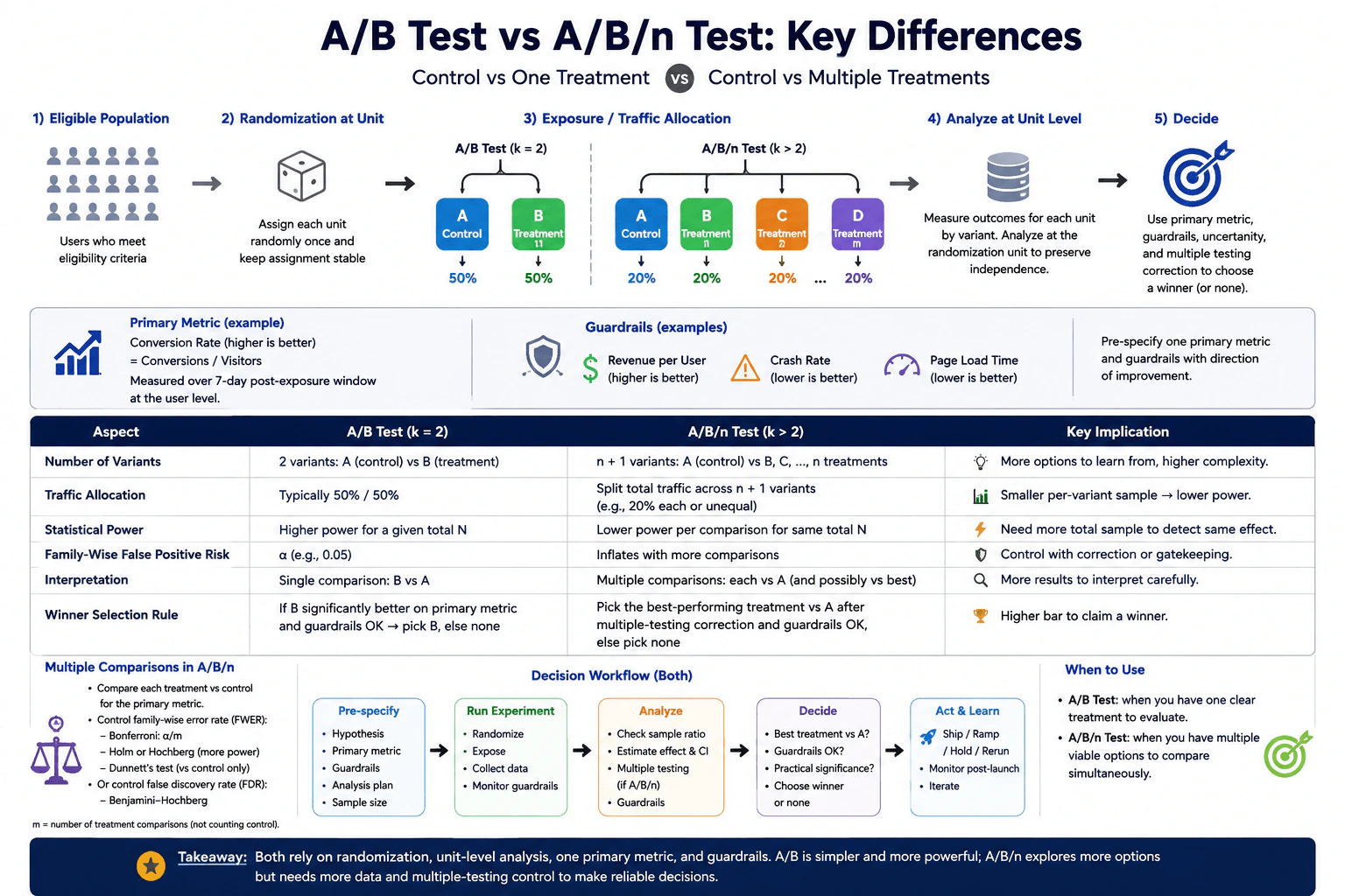
What is the difference between an A/B test and an A/B/n test? diagram
How to Explain It in an Interview

Start with the structure. In an A/B test, each eligible unit is randomized to A, the control, or B, one treatment. A common allocation is 50% to A and 50% to B. In an A/B/n test, the same stable-randomization idea is extended to more than two variants. The diagram shows a control plus several treatments. Traffic can be split equally or unequally, but every unit should remain in its assigned variant and see only that assigned experience.

Analyze outcomes at the same unit used for randomization. Pre-specify one primary metric and its direction of improvement. The approved diagram uses conversion rate as an example, defined as conversions divided by visitors and measured over a 7-day post-exposure window at the user level. It also shows guardrails such as revenue per user, crash rate, and page load time. A candidate treatment should not be selected if an important guardrail becomes unacceptable.

The first major difference is statistical power. If total sample size stays fixed, an A/B test concentrates observations into two groups. An A/B/n test spreads the same traffic across more groups. Each variant therefore usually receives fewer observations, confidence intervals become wider, and power for each treatment-versus-control comparison falls. To detect the same effect with similar power, an A/B/n experiment often needs more total sample.

The second major difference is family-wise false-positive risk. In a basic A/B test, the main comparison is B versus A. In an A/B/n test, several treatments may each be compared with the same control. As the number of comparisons increases, the probability that at least one treatment appears significant by chance also increases. If the decision depends on those comparisons, use a pre-specified multiple-testing method such as Bonferroni, Holm, or an appropriate control-versus-many procedure. False discovery rate control can serve a different objective, but it is not the same as controlling family-wise error.

Before interpreting treatment effects, check whether the observed assignment counts are compatible with the planned traffic split. A serious sample-ratio mismatch can indicate a problem in randomization, eligibility, exposure logging, or the analysis pipeline. Investigate that problem before trusting the effect estimates.

Then report effect size and uncertainty, not only whether a p-value crosses a threshold. For an A/B test, choose B only if it beats A on the primary metric by a practically meaningful amount, the uncertainty is acceptable, and all important guardrails remain acceptable. Otherwise choose no winner, hold, or rerun.

For an A/B/n test, first apply the pre-specified multiple-testing procedure to the treatment-versus-control comparisons. Then identify treatments that validly beat the control, check guardrails and practical significance, and choose the best qualifying treatment according to the pre-specified rule. If no treatment qualifies, choose no winner instead of forcing a selection.

The interview takeaway is that A/B is simpler to power and interpret because there is one treatment comparison. A/B/n can evaluate several viable options in one experiment, but it divides traffic across more arms, increases statistical and interpretive complexity, and requires explicit multiple-testing control and a disciplined winner-selection rule.

Technical Approach
  1. Define the eligible population and experimental unit.
  2. Randomize each unit once and keep treatment assignment stable.
  3. For A/B, assign units to one control and one treatment; for A/B/n, assign units to one control and multiple treatments.
  4. Pre-specify the traffic-allocation ratio for all variants.
  5. Pre-specify one primary metric, including its numerator, denominator, direction of improvement, analysis window, and observation grain.
  6. Pre-specify important guardrails and the rule that determines whether a guardrail failure blocks shipping.
  7. Plan sample size and power using the number of variants and comparisons because more variants reduce per-variant sample when total traffic is fixed.
  8. Run the experiment and expose each unit only to its assigned variant.
  9. Check observed allocation for sample-ratio mismatch before interpreting treatment effects.
  10. Estimate treatment-versus-control effects and uncertainty at the randomization-unit level.
  11. For A/B/n, apply the pre-specified multiple-comparison procedure before selecting a winner.
  12. Evaluate the primary metric, guardrails, uncertainty, and practical significance.
  13. Select the best qualifying treatment using the pre-specified winner rule, or choose no winner and hold or rerun.
Practical Insights

A/B is statistically simpler because there is usually one treatment-versus-control comparison. With the same total number of units, each of its two groups gets more data, so it usually has more power than an A/B/n design with many groups. A/B/n can compare several options at once, but traffic is divided more ways. That gives smaller samples per variant, wider uncertainty, and often a need for more total traffic. More comparisons also create more opportunities for false positives, so the analysis and winner-selection rule require stronger error control and more careful interpretation.

Why Interviewers Ask This

Interviewers want to see whether you understand that adding experiment variants changes both design and statistical reasoning. A strong answer connects stable randomization, exposure, traffic allocation, primary metrics, guardrails, statistical power, multiple-comparison risk, effect uncertainty, and the rule used to select a winner.

Common interview mistakes

Common mistakes are treating A/B/n as merely an A/B test with extra arms; ignoring the loss of per-variant power when total traffic is fixed; picking the treatment with the largest observed lift without accounting for uncertainty; running many treatment-versus-control tests without controlling family-wise false-positive risk; changing the primary metric or winner rule after seeing results; analyzing at a different grain from the randomization unit; ignoring sample-ratio mismatch; repeatedly peeking at fixed-horizon p-values; and selecting a treatment even when important guardrails fail.

Interview tip

Lead with the one-sentence distinction, then explain the consequences of adding variants in this order: traffic per arm, power, multiple-testing risk, interpretation, and winner selection. Mention that both designs still require stable randomization, one pre-specified primary metric, guardrails, effect sizes, uncertainty, and the option to choose no winner.
Interviewer may ask next
What should you do if the observed traffic split is very different from the planned allocation?

Treat it as a possible sample-ratio mismatch and investigate it before interpreting treatment effects. Check randomization and assignment logic, eligibility filtering, exposure logging, missing observations, and the analysis pipeline. A large unexplained mismatch can mean the experiment groups are not being observed as intended, so even an apparently significant treatment result should not be trusted until the mismatch is understood.

What changes if total traffic is fixed but you increase the number of treatments in the A/B/n test?

Each variant usually receives fewer units, so standard errors become larger and power for each treatment-versus-control comparison falls. At the same time, the number of comparisons grows, which increases family-wise false-positive risk if multiplicity is not controlled. You may therefore need more total sample, fewer treatments, or a different allocation strategy. The winner rule should still use the pre-specified primary metric, multiple-testing procedure, guardrails, uncertainty, and practical value, with no winner allowed if no treatment qualifies.

52. What are guardrail metrics in an experiment?ExperimentationEasy

Question Details

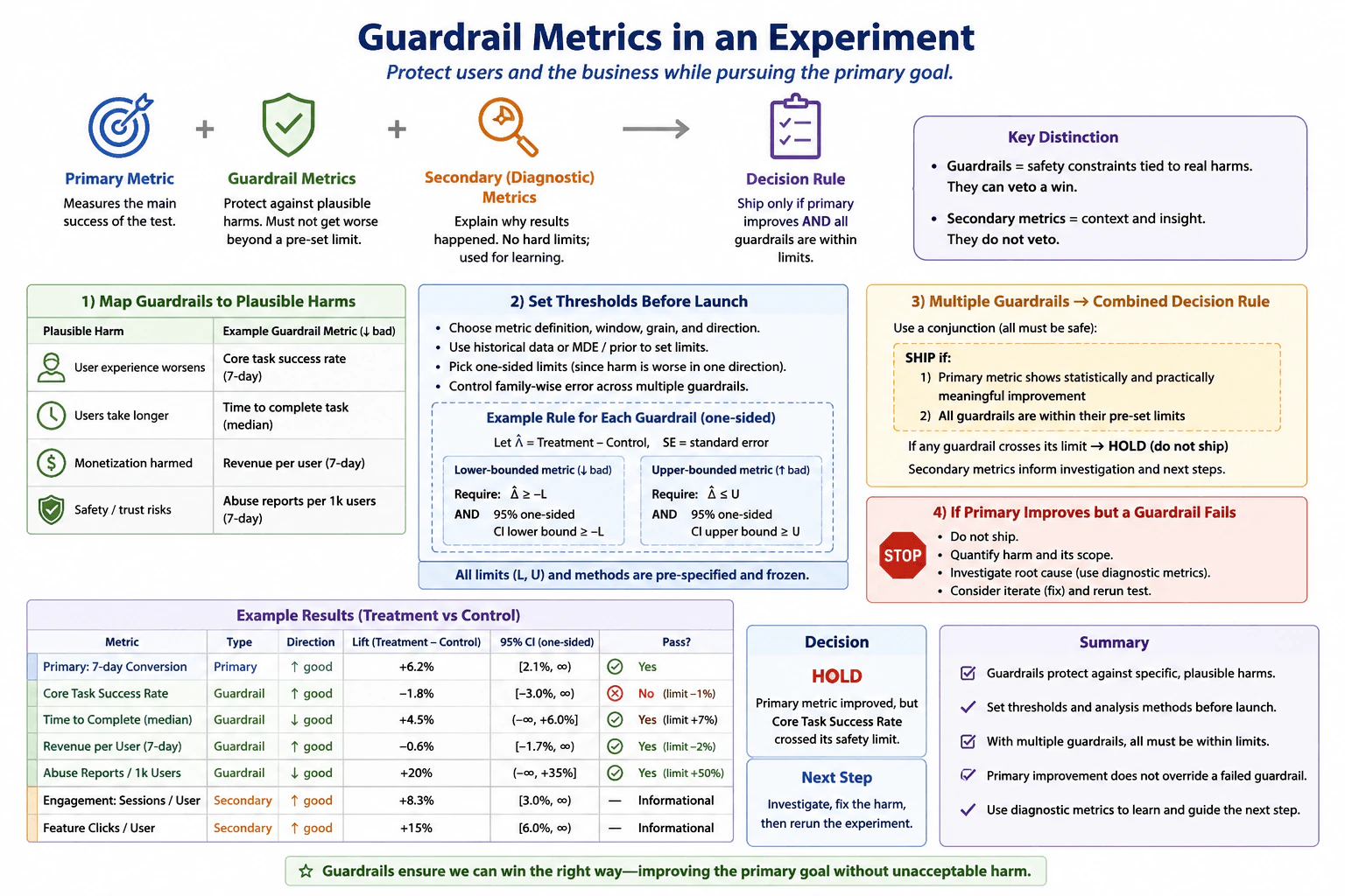
A team has one primary success metric for a randomized product test. Define guardrail metrics and distinguish them from secondary diagnostic metrics. Explain how guardrails should map to plausible harms, how thresholds are set before launch, how multiple guardrails affect the decision rule, and what to do when the primary metric improves but a guardrail crosses its limit.

Short Interview Answer (30-60 seconds)

Guardrail metrics are pre-set safety constraints tied to plausible harms. Unlike secondary diagnostic metrics, they can veto a win. Define their direction and acceptable limits before launch. With several guardrails, require all to pass. If the primary metric improves but one guardrail crosses its limit, hold the launch and investigate.

Detailed Explanation

Guardrail metrics protect users or the business while an experiment pursues its primary goal. They are defined before launch and tied to specific plausible harms, such as a worse core experience, slower task completion, lower monetization, or greater safety risk. Each guardrail has a defined direction and a pre-set acceptable degradation limit. Secondary diagnostic metrics are different: they help explain why the experiment changed behavior, but they normally do not have hard veto thresholds. With several guardrails, the decision rule is conjunctive: the primary metric must improve meaningfully and every required guardrail must stay within its pre-set safe region.

Useful Questions to Ask the Interviewer
  1. What user or business harms are important enough to block a launch?
  2. How is each guardrail defined, including its grain, analysis window, denominator when applicable, and direction of improvement?
  3. What historical data, prior evidence, or practical tolerance should be used to set each acceptable degradation limit?
  4. When several guardrails determine the decision, should we require every one to pass and how should uncertainty across those tests be handled?
What are guardrail metrics in an experiment? diagram
How to Explain It in an Interview

Start with the roles of the metrics. The primary metric measures the main success of the experiment. A guardrail metric limits how much harm we are willing to accept while pursuing that success. A secondary diagnostic metric helps explain what happened, but normally does not veto the launch.

Guardrails should map directly to plausible harms. For example, if a treatment could make the main task harder, core task success rate can be a guardrail. If it could slow users down, median time to complete the task can be a guardrail. If monetization could be harmed, revenue per user can be monitored. If trust or safety could worsen, a measure such as abuse reports per 1,000 users can be monitored. The important point is that every guardrail should exist because it protects against a specific meaningful harm.

Before launch, define each guardrail completely. Specify its metric definition, grain, analysis window, denominator when applicable, and direction of improvement. Then choose the largest degradation that is still acceptable. Historical data, prior evidence, domain knowledge, and practical business judgment can help set that limit. The threshold and analysis method should be frozen before looking at experiment results so the team does not move the goalposts after seeing the data.

Because guardrails usually protect against harm in one direction, a one-sided safety rule is often appropriate. Let the estimated effect be treatment minus control. For a metric where a decrease is harmful, require the effect and its uncertainty to stay above the pre-specified lower safety limit. For a metric where an increase is harmful, require the effect and its uncertainty to stay below the pre-specified upper safety limit. Report the effect size and confidence interval rather than relying only on a significance label.

If several guardrails jointly determine whether the experiment can ship, the launch rule should require all of them to remain within their limits. This is an AND rule, not a vote. One guardrail failure is enough to hold the launch because guardrails are constraints on unacceptable harm. When many statistical tests jointly drive the decision, pre-specify an appropriate multiple-comparison approach, such as controlling family-wise error, so the safety decision does not become too sensitive to random noise.

If the primary metric improves but a guardrail crosses its limit, do not ship or ramp simply because the primary result is attractive. Hold the decision. Quantify the harm and its uncertainty, identify where it occurs, and use secondary diagnostic metrics to investigate why it happened. If possible, change the treatment to remove or reduce the harm. Then rerun the experiment and reconsider shipping only after the primary benefit and all required guardrails are revalidated.

Technical Approach
  1. Define the primary success metric and what counts as a meaningful improvement.
  2. List plausible user and business harms caused by the treatment.
  3. Map each material harm to a measurable guardrail metric.
  4. Define each guardrail's grain, window, denominator when applicable, and direction of improvement.
  5. Set a pre-launch acceptable degradation limit for each guardrail using historical data, prior evidence, domain knowledge, and practical tolerance.
  6. Pre-specify the statistical safety rule, including one-sided limits when appropriate and a multiple-comparison method when several guardrails jointly determine the decision.
  7. Run the randomized experiment and estimate treatment-minus-control effects with uncertainty for the primary metric and guardrails.
  8. Ship or ramp only if the primary metric improves meaningfully and every required guardrail remains within its pre-set limit.
  9. If any guardrail fails, hold the launch, quantify and diagnose the harm using secondary metrics, mitigate the cause, and rerun the experiment before reconsidering shipment.
Practical Insights

Guardrails reduce the risk of shipping a change that wins on one metric while causing important harm elsewhere. The tradeoff is that every extra guardrail adds measurement work and makes the combined decision harder to pass. With many guardrails, random noise can also create more apparent failures, so the statistical method should account for multiple tests when they jointly control the decision. Very strict thresholds may block useful changes, while very loose thresholds may allow unacceptable harm. Good guardrails focus on material risks and use stable definitions and pre-set limits.

Why Interviewers Ask This

Interviewers want to know whether you can optimize a primary metric without ignoring important side effects. They are testing whether you can distinguish guardrails from diagnostic metrics, connect each guardrail to a plausible harm, set decision thresholds before seeing results, reason about several guardrails together, use uncertainty correctly, and make a disciplined ship-or-hold decision when the primary metric and safety constraints disagree.

Common interview mistakes

Common mistakes are treating every secondary metric as a guardrail, choosing guardrails that are not tied to plausible harms, changing thresholds after seeing results, failing to define the harmful direction, ignoring effect uncertainty, using many guardrails without considering multiple-comparison risk, treating guardrails as a majority vote instead of requiring all important constraints to pass, and shipping because the primary metric improved even though a guardrail crossed its pre-set limit.

Interview tip

State the distinction in one clean sentence: the primary metric measures the win, guardrails constrain unacceptable harm, and secondary metrics explain what happened. Then give the decision rule clearly: ship only when the primary result is meaningful and every required guardrail remains within its pre-set limit.

Interviewer may ask next
How would you set a guardrail threshold when the metric naturally varies from week to week?

First define the metric, grain, analysis window, denominator when applicable, and harmful direction. Then use historical data to understand its normal variation and combine that with prior evidence, domain knowledge, and the largest practical degradation the team is willing to accept. Pre-specify the safety limit and the uncertainty rule before launch. If several guardrails jointly control the decision, also pre-specify how multiple comparisons will be handled rather than changing the method after seeing results.

What if the primary metric improves strongly, but only one of several guardrails barely crosses its limit?

If the pre-specified rule requires all guardrails to stay within their limits, the correct decision is to hold rather than ship. I would quantify how far that guardrail crossed the limit and examine its confidence interval, then use secondary diagnostic metrics to understand where and why the harm occurred. I would not relax the threshold because the primary result is strong. If the harm can be mitigated, I would change the treatment and rerun the experiment so the primary benefit and all required guardrails can be revalidated together.

53. Why is repeatedly peeking at fixed-horizon A/B test results a problem?ExperimentationMedium

Question Details

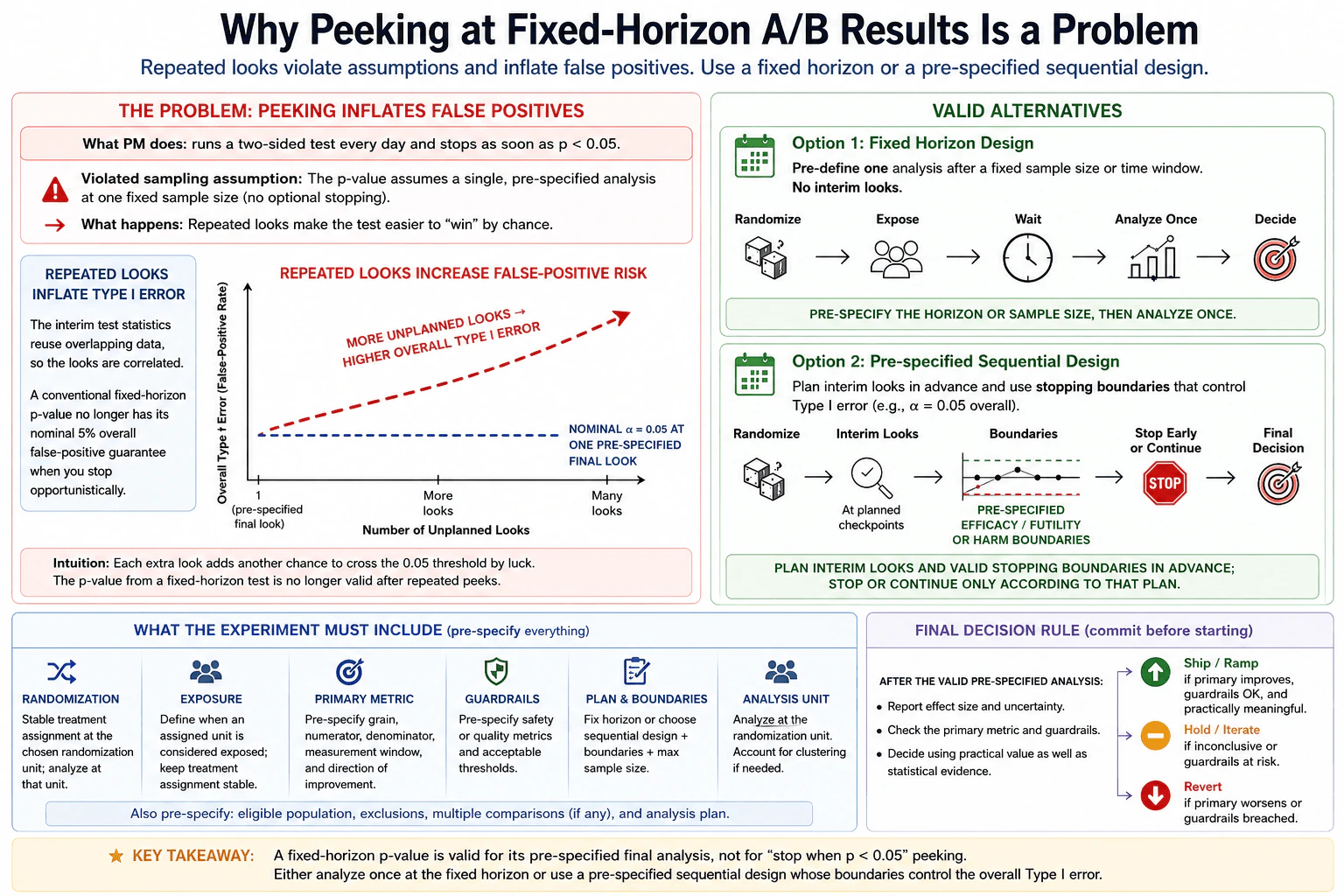
A product manager checks a conventional two-sided significance test every day and wants to stop as soon as p<0.05. Explain which sampling assumption is violated and how repeated looks affect the false-positive rate. Define a valid alternative using a fixed horizon or a pre-specified sequential design, including randomization, exposure, primary metric, guardrails, stopping boundaries, and the final decision rule.

Short Interview Answer (30-60 seconds)

A fixed-horizon p-value is calibrated for a pre-specified final analysis. If I check repeatedly and stop when p < 0.05, optional stopping makes the overall false-positive rate exceed its nominal 5% guarantee. I would either analyze once at the fixed horizon or use a pre-specified sequential design with valid stopping boundaries.

Detailed Explanation

A conventional fixed-horizon A/B test is designed around a pre-specified final analysis. If a product manager checks accumulating results every day and stops the first time p < 0.05, the stopping rule has changed into optional stopping. Random fluctuations under the null can temporarily look significant, and every additional unplanned look gives another opportunity to stop on one of those fluctuations. Because the cumulative interim statistics reuse overlapping data, the looks are correlated. The result is that a nominal 0.05 threshold no longer guarantees a 5% overall Type I error rate.

Useful Questions to Ask the Interviewer
  1. Is the experiment intended to have one fixed final analysis, or is valid early stopping required?
  2. What is the randomization unit, and should the analysis use that unit directly or account for clustering?
  3. How is exposure defined for an assigned experimental unit?
  4. What exactly is the primary metric, including grain, numerator, denominator, measurement window, and direction of improvement?
  5. Which guardrail metrics and acceptable thresholds must be checked before the final decision?
  6. If this is sequential, which interim looks and stopping boundaries will be specified before launch?
Why is repeatedly peeking at fixed-horizon A/B test results a problem? diagram
How to Explain It in an Interview

Start with the sampling plan. A conventional fixed-horizon test is calibrated for a pre-specified final analysis, such as a chosen sample-size horizon or time horizon. The important problem is not simply viewing a dashboard. The problem is using unplanned interim results to decide whether to stop the experiment.

Suppose the null hypothesis is true. Random noise can make the treatment look favorable at some interim point. If the product manager keeps testing and stops at the first ordinary fixed-horizon p-value below 0.05, each unplanned look provides another opportunity for a false rejection. Therefore, the overall probability of at least one false positive becomes larger than the nominal 5% level.

The repeated cumulative test statistics are correlated because later analyses reuse much of the same data from earlier analyses. For that reason, I would not use the independent-look formula 1 - (1 - alpha)^k as an exact false-positive calculation for these cumulative A/B looks. The defensible conclusion is that opportunistic repeated testing invalidates the conventional fixed-horizon Type I error guarantee and increases false-positive risk.

There are two valid alternatives.

First, use a fixed-horizon design. Before launch, choose the horizon or sample size. Keep treatment assignment stable at the chosen randomization unit and analyze at that unit, accounting for clustering if needed. Define when an assigned unit counts as exposed. Pre-specify the primary metric, including its grain, numerator, denominator, measurement window, and direction of improvement. Also pre-specify safety or quality guardrails and their acceptable thresholds. Then wait until the planned horizon and perform the conventional two-sided analysis once.

Second, if early stopping is genuinely useful, use a pre-specified sequential design. Decide the interim checkpoints before the experiment begins. Use statistical stopping boundaries designed to control the overall Type I error across those planned looks. The plan may include efficacy boundaries and, when appropriate, futility or harm boundaries. At each planned checkpoint, compare the accumulated evidence with those boundaries and stop or continue only according to the pre-specified rule.

For either design, the assignment and exposure rules must remain stable. The analysis should respect the randomization unit. If observations are clustered or units interfere with one another, the analysis must account for that dependence rather than treating all observations as independent.

Before interpreting the treatment effect, check experiment integrity. If an allocation ratio was specified, diagnose sample-ratio mismatch before trusting the effect estimate. Pre-specify the main analysis and material exclusions. If the final decision depends on multiple hypothesis tests, use an appropriate pre-specified multiple-comparison procedure.

The final business decision should not be based only on whether p < 0.05. After the valid pre-specified analysis, report the treatment effect and its uncertainty. Check the primary metric and the guardrails, then consider practical value. Ship or ramp when the primary metric improves enough to matter and guardrails remain acceptable. Hold, iterate, or rerun when evidence is inconclusive. Revert when the primary outcome worsens materially or a guardrail is breached.

Technical Approach
  1. Choose the testing framework before observing results: fixed horizon or pre-specified sequential testing.
  2. Define the randomization unit and keep treatment assignment stable.
  3. Define when an assigned unit is considered exposed.
  4. Pre-specify the primary metric: grain, numerator, denominator, measurement window, and direction of improvement.
  5. Pre-specify guardrail metrics and acceptable thresholds.
  6. For a fixed-horizon design, pre-specify the horizon or sample size and perform the conventional two-sided analysis once at the planned end.
  7. For a sequential design, pre-specify interim checkpoints and stopping boundaries that control the overall Type I error.
  8. At each permitted analysis, follow only the pre-specified stopping rule; do not stop merely because an ordinary fixed-horizon p-value falls below 0.05.
  9. Check experiment integrity, including sample-ratio mismatch when an allocation ratio is specified, before interpreting the effect.
  10. Report effect size and uncertainty, check the primary metric and guardrails, and make the ship, ramp, hold, rerun, or revert decision using statistical evidence and practical value.
Practical Insights

A fixed-horizon design is simpler to plan and explain, but it does not allow valid significance-driven early stopping with ordinary fixed-horizon p-values. A sequential design can support valid early stopping, but the interim looks and boundaries must be planned in advance. Early stopping may require stronger evidence at some checkpoints to preserve the overall false-positive rate. The main cost is not computation. It is disciplined experimental planning, correct metric definitions, stable assignment, guardrail monitoring, and resisting data-dependent changes after results are visible.

Why Interviewers Ask This

Interviewers want to see whether you understand that the stopping rule is part of experimental design. They are testing whether you can distinguish a conventional fixed-horizon test from a valid sequential test, explain why opportunistic peeking inflates false positives, define randomization, exposure, metrics and guardrails before launch, and make the final decision using effect size, uncertainty, practical value, and safety rather than significance alone.

Common interview mistakes

Common mistakes are checking a conventional p-value repeatedly and stopping at the first p < 0.05; treating cumulative interim looks as independent; using 1 - (1 - alpha)^k as an exact calculation for correlated cumulative looks; changing the stopping rule after seeing results; calling ordinary repeated fixed-horizon testing a sequential test; failing to pre-specify the randomization unit, exposure rule, primary metric, guardrails, or analysis plan; ignoring sample-ratio mismatch; reporting significance without effect size and uncertainty; and shipping automatically because p < 0.05 even when the practical effect is too small or guardrails are unacceptable.

Interview tip

Lead with the key distinction: a fixed-horizon p-value is calibrated for its pre-specified final analysis, not for 'stop when p < 0.05' peeking. Then describe the two valid alternatives and finish with the decision rule: effect size, uncertainty, primary metric, guardrails, and practical value.

Interviewer may ask next
What if the product manager looks at the dashboard every day but promises not to stop or change the experiment until the pre-specified horizon?

Simply viewing interim data does not by itself invalidate the final fixed-horizon test. The problem arises when the interim results affect stopping, continuation, exclusions, metric selection, or other analysis choices. If the original horizon and analysis plan truly remain unchanged and the decision-making test is performed at the pre-specified end, the conventional fixed-horizon procedure can retain its intended Type I error control. In practice, teams should document the rule clearly because seeing interim results can create pressure to change the plan.

What if the business genuinely needs to stop early because continuing the experiment is costly or a guardrail may be harmed?

Then I would use a sequential design planned before launch rather than repeatedly applying an ordinary fixed-horizon p-value. I would pre-specify the interim checkpoints and valid stopping boundaries, including efficacy and any needed futility or harm rules. Those boundaries should control the intended overall Type I error across the planned looks. At each checkpoint, we stop or continue only according to that rule. The final business action still depends on the treatment effect, uncertainty, primary metric, guardrails, and practical value.

54. How would you control the multiple-comparisons problem in an experiment?ExperimentationMedium

Question Details

A randomized test has one control, four treatment variants, and several outcomes. Define the family of hypotheses that will influence the decision, the primary comparison, randomization and exposure units, and the desired error guarantee. Compare family-wise and false-discovery-rate controls, explain the effect on power, and state how the corrected results and guardrails determine which variant, if any, ships.

Short Interview Answer (30-60 seconds)

I would pre-specify the decision-driving hypothesis family and error guarantee before seeing results. I would use Holm for FWER when any false primary win is costly, or Benjamini-Hochberg for FDR when some false discoveries are acceptable. I would ship only a corrected primary winner that also passes guardrails and practical-value checks.

Detailed Explanation

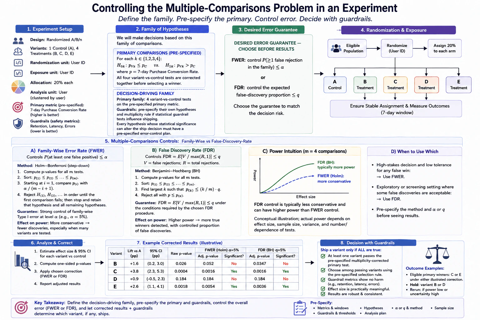
The key is to define the decision before looking at p-values. In this test, one control is compared with four treatment variants. The pre-specified primary metric is the 7-day Purchase Conversion Rate, measured at the user level, and the primary family contains the four treatment-versus-control hypotheses. Users are randomized with stable assignment, with 20% allocated to each arm, and the analysis stays at the user randomization unit. Before results are examined, I choose whether the decision needs family-wise error control or false-discovery-rate control, then use corrected evidence plus guardrails to decide whether any variant ships.

Useful Questions to Ask the Interviewer
  1. Which hypotheses can directly change the ship decision, and should primary and statistical guardrail hypotheses use separate pre-specified multiplicity families?
  2. Is the decision high-stakes enough that we need strong protection against even one false primary win, or is a controlled proportion of false discoveries acceptable?
  3. Is the 7-day Purchase Conversion Rate the single pre-specified primary metric, with user as its analysis grain and higher values considered better?
  4. Are users randomized and exposed consistently at the user level, with stable assignment and 20% allocation to each of the five arms?
  5. What practical-effect threshold, guardrail thresholds, sample size, power target, analysis window, and stopping rule were pre-specified before launch?
How would you control the multiple-comparisons problem in an experiment? diagram
How to Explain It in an Interview

Start with the decision-driving family. For the primary metric, define four treatment-versus-control comparisons before seeing results. For each treatment Vk, where k is 1 through 4, test H0k: pVk <= pC against H1k: pVk > pC, where p is the 7-day Purchase Conversion Rate. Correct these four tests together before selecting a winner. If statistical guardrail hypotheses can independently change shipping, pre-specify those hypotheses and their multiplicity rule too instead of adding them after seeing the results.

Next choose the error guarantee. Family-wise error rate, or FWER, controls the probability of at least one false rejection in the family. A step-down Holm procedure is appropriate when a false primary win is costly. Compute all m p-values, sort them from smallest to largest, then compare p(i) with alpha divided by m - i + 1. Reject hypotheses in order until the first comparison fails, then stop and retain that hypothesis and all remaining hypotheses. This gives strong family-wise Type I error control at the chosen alpha level.

False discovery rate, or FDR, answers a different question. Let V be the number of false rejections and R be the total number of rejections. Then FDR is E[V / max(R, 1)]. Benjamini-Hochberg sorts the p-values, finds the largest k satisfying p(k) <= (k/m)q, and rejects hypotheses through k under the conditions required by the procedure. FDR is usually less conservative than FWER, so it can identify more true effects, but it accepts a controlled risk that some discoveries are false.

That creates the main power tradeoff. FWER control is more conservative, so real improvements can be harder to detect. FDR control is typically less conservative and can have higher power. Actual power depends on effect size, sample size, variance, and the number and dependence structure of the tests. I would therefore choose the error guarantee, sample size, power target, and stopping rule before the experiment rather than changing them after seeing the results.

The experimental mechanics also matter. Eligible users receive stable user-level assignment. There is one control and four treatments, with 20% allocated to each arm. The randomization unit and exposure unit are the user, and outcomes are analyzed at the user level over the 7-day window. I would estimate each treatment effect versus control and report its confidence interval together with the corrected significance result. I would also check experiment validity, including sample-ratio mismatch, data quality, interference or contamination when relevant, and the pre-specified stopping rule. With fixed-horizon p-values, I would not repeatedly peek and stop only when significance appears.

Finally, corrected significance is necessary but not sufficient for shipping. At least one variant must pass the pre-specified multiplicity-corrected primary test. If several variants pass, choose among them using the pre-specified selection rule instead of picking whichever result looks best after the fact. The chosen candidate must also have a practically meaningful effect and no unacceptable guardrail harm, such as worse retention, latency, or errors. If no variant meets those conditions, hold. If uncertainty remains high or the experiment has insufficient power, rerun rather than declaring a winner.

Technical Approach
  1. Define the ship decision and list every statistical hypothesis that can change it.
  2. Pre-specify the primary family as the four treatment-versus-control tests on the 7-day Purchase Conversion Rate.
  3. Pre-specify any statistical guardrail hypotheses and their multiplicity rule if those tests can block shipping.
  4. Keep stable user-level randomization and exposure, allocate 20% to each arm, and analyze at the user level.
  5. Choose the error guarantee before seeing results: FWER for strong protection against any false primary win, or FDR when a controlled false-discovery proportion is acceptable.
  6. Estimate each treatment effect versus control, its uncertainty, and its p-value.
  7. For FWER, apply the Holm step-down procedure. For FDR, apply Benjamini-Hochberg under its required conditions.
  8. Check experiment validity, including sample-ratio mismatch, data quality, interference or contamination when relevant, and the pre-specified stopping rule.
  9. Identify variants that pass the chosen multiplicity correction on the primary family.
  10. If several pass, apply the pre-specified selection rule.
  11. Require acceptable guardrails, practical value, and adequate uncertainty before shipping. Otherwise hold or rerun.
Practical Insights

The main statistical cost of controlling many comparisons is lower power. FWER is stricter because it protects against even one false rejection in the family, so real improvements can be harder to detect. FDR is usually less conservative and can find more true effects, but some rejected hypotheses may be false discoveries. Testing more hypotheses increases the multiplicity burden. Larger samples can recover power, but they require more traffic and time. Operationally, the difficult part is often governance: defining the family, metrics, thresholds, sample size, error guarantee, and stopping rule before results are visible.

Why Interviewers Ask This

This tests whether the candidate understands that testing several variants or outcomes increases the chance of false discoveries and that the correction method must match the decision risk. It also tests whether the candidate can define a hypothesis family before seeing results, preserve valid randomization and analysis units, distinguish FWER from FDR, explain the power tradeoff, and combine corrected statistical evidence with guardrails and practical significance when deciding whether any variant should ship.

Common interview mistakes

Common mistakes are testing every variant and outcome independently at the original significance threshold; defining the hypothesis family only after seeing which results look promising; choosing the empirically best variant before correcting the four treatment-versus-control tests; treating FWER and FDR as the same guarantee; choosing FDR only because there are many tests without considering the decision risk; claiming that FDR always has higher power; adding metrics or changing guardrails after seeing results; ignoring sample-ratio mismatch or unstable assignment; analyzing at a finer grain than the randomization unit without accounting for dependence; repeatedly peeking at fixed-horizon p-values; reporting only significance without effect size and uncertainty; and shipping a statistically significant variant that violates guardrails or has little practical value.

Interview tip

Lead with the hypothesis family and the desired error guarantee, not with a correction formula. Explain what is being tested, why those tests belong together, when you would choose FWER versus FDR, and how corrected primary evidence, guardrails, uncertainty, and practical value combine into the ship decision.

Interviewer may ask next
What if the guardrail metrics are also tested statistically and any significant guardrail harm can block shipping?

Then I would pre-specify those guardrail hypotheses and their error-control rule before the experiment. I would not silently add them to the primary family after seeing results. Depending on the decision policy, the primary and guardrail hypotheses can use separate pre-specified families or a structured multiplicity procedure. The important point is that every statistical hypothesis capable of changing the shipping decision has an explicit error-control plan. A variant must still pass the corrected primary test and satisfy the guardrail rule before it is eligible to ship.

What changes if FWER control leaves the experiment with too little power to detect a practically important effect?

I would not switch to a looser correction after seeing the results. Before launch, I would quantify the required power for the pre-specified primary family and increase sample size or duration if needed, reduce unnecessary decision-driving hypotheses, or reconsider whether the decision risk truly requires FWER rather than FDR. If the experiment has already run and is underpowered, an inconclusive corrected result should normally lead to hold or rerun, not to an uncorrected winner.

55. A randomization bug sent 60% of traffic to treatment. Is the experiment salvageable?ExperimentationHard

Question Details

For an intended user-randomized A/B test, distinguish a purely random unequal allocation from a systematic assignment or logging failure. Compare assigned and exposed populations, test sample ratios, examine pre-treatment covariates and missing outcomes, and trace the bug's mechanism. State how unequal allocation changes variance, when unbiased analysis remains possible, when adjustment is insufficient, and the criteria for discarding and rerunning the test.

Short Interview Answer (30-60 seconds)

Yes, if the 60/40 split was still random. I would verify assignment, exposure, logging, pre-treatment balance, and missingness first. If those checks pass, analyze the unequal allocation with the actual group sizes. If assignment became systematic or the data cannot support a causal comparison, discard and rerun.

Detailed Explanation

A 60/40 split is not automatically fatal. The key question is why it happened. If each eligible user was still independently randomized, but the treatment probability became 60% instead of the planned 50%, the causal comparison can remain unbiased and the main cost is lower precision. If the bug instead made assignment depend on user attributes, changed exposure after assignment, caused group-specific logging failures, or produced problematic missing outcomes, causal validity may be broken. I would diagnose the mechanism before interpreting any treatment effect and then decide whether to salvage, adjust, or rerun.

Useful Questions to Ask the Interviewer
  1. Was the intended randomization unit the user, with a planned 50/50 treatment-control allocation?
  2. Do we have both assignment logs and actual exposure logs for the same users?
  3. Did users keep a stable assignment, or could their assigned arm change during the experiment?
  4. Can we locate where the 60/40 deviation first appeared: assignment, exposure, logging, or outcome collection?
  5. Are pre-treatment user attributes available for comparing the assigned treatment and control arms?
  6. Are outcomes missing at similar rates across the assigned groups?
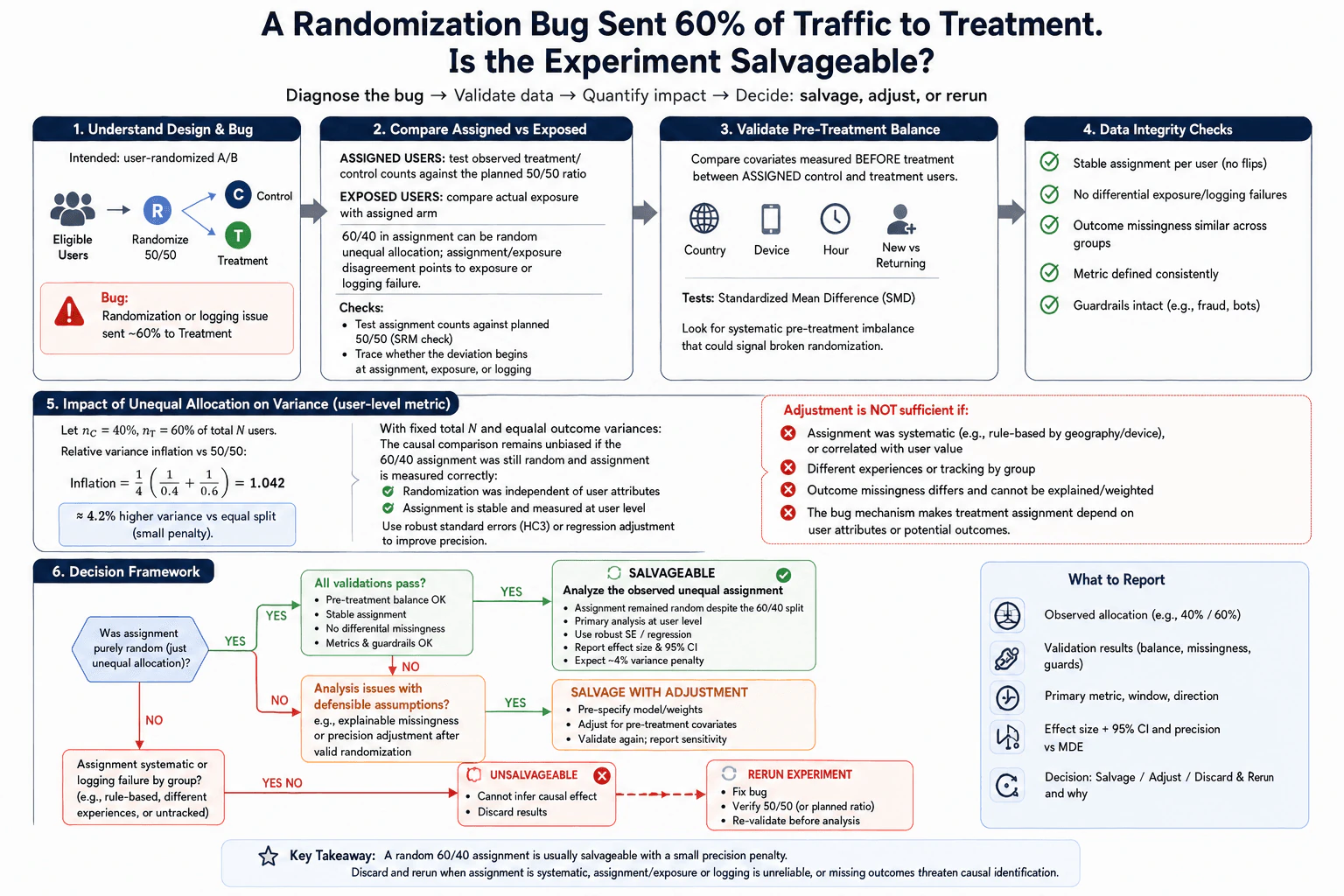
A randomization bug sent 60% of traffic to treatment. Is the experiment salvageable? diagram
How to Explain It in an Interview

Start at the randomization unit. This is an intended user-randomized A/B test, so I would reconstruct the user-level path from eligible user to assigned arm to actual exposure to observed outcome. I would not interpret the treatment effect until that path is understood.

First, test the observed assignment counts against the planned 50/50 allocation. This is a sample-ratio-mismatch, or SRM, check. A clear 60/40 assignment will normally fail a test against the planned 50/50 ratio in a sufficiently large experiment. That confirms the planned allocation was not followed, but it does not by itself prove biased randomization. I still need to understand the bug mechanism.

Next, compare assigned users with exposed users. If about 60% of users were randomly assigned treatment and actual exposure follows assignment consistently, the experiment may still be valid. If assignment and exposure disagree by group, or assignment looks correct while exposure or logging produces the 60/40 pattern, I would investigate an implementation, exposure, or logging failure.

Then compare pre-treatment covariates between the assigned treatment and control arms. These are variables measured before treatment, such as device type or other user characteristics already available before randomization. Standardized mean differences can be useful diagnostics. I would look for broad or systematic imbalance that could signal broken randomization. Balance does not prove randomization was correct, because chance imbalance is possible and unobserved variables may still differ.

I would also check whether outcome missingness differs across assigned arms. Similar missingness is reassuring. Differential missingness is dangerous because treatment and control may then represent different observed subsets. If the missingness can be handled under explicit, defensible assumptions, weighting or another pre-specified adjustment may be reasonable. If it is unexplained and plausibly related to treatment or outcomes, adjustment is not enough to restore a trustworthy causal comparison.

For a genuinely random 60/40 allocation, I would analyze using the actual group sizes. With fixed total sample size N, control fraction 0.4, treatment fraction 0.6, and equal outcome variances, the variance of a difference in means is proportional to 1/n_C + 1/n_T. Relative to 50/50, the variance inflation is (1/4) × (1/0.4 + 1/0.6) = 1.0417. That is about 4.2% higher variance, so the loss of precision is small under those assumptions.

If the group outcome variances are not equal, I would not rely on the 4.2% shortcut. I would use the actual group sizes and an appropriate robust or unequal-variance standard error. Regression adjustment using pre-treatment variables can also improve precision after valid randomization, but it cannot repair a fundamentally non-random assignment mechanism.

The primary causal analysis should remain at the user randomization level and follow the assigned arm when randomization is valid. I would report the observed allocation, the SRM diagnosis, assignment-versus-exposure checks, pre-treatment balance, missingness checks, the primary metric definition and analysis window if they were pre-specified, effect size, confidence interval, sample sizes, and any justified adjustment. Guardrail checks should also remain consistent with the original experiment design.

Adjustment is not sufficient when the bug made treatment assignment systematic, such as rule-based assignment by geography, device, user value, or another attribute related to potential outcomes; when groups had different experiences or tracking; when assignment cannot be reconstructed reliably; or when outcome missingness differs in a way that cannot be credibly explained or modeled.

The final decision is therefore conditional. Salvage and analyze the experiment when the observed 60/40 assignment remained random, assignments were stable, exposure and logging are trustworthy, pre-treatment diagnostics do not reveal evidence of a broken mechanism, and outcome collection supports the intended comparison. Use adjustment only when its assumptions are defensible after valid randomization. Discard the causal result and rerun when assignment is systematic or the assignment, exposure, logging, or missing-outcome process prevents credible causal identification. Before rerunning, fix the bug and verify the planned allocation and data pipeline.

Technical Approach
  1. Confirm that the intended experiment was user-randomized with a planned 50/50 allocation.
  2. Reconstruct the user-level path: eligible user -> assigned arm -> actual exposure -> observed outcome.
  3. Test observed assignment counts against the planned 50/50 ratio to diagnose SRM.
  4. Compare assigned and exposed populations to locate whether the deviation begins at assignment, exposure, or logging.
  5. Verify stable assignment and trace whether the bug mechanism depends on user attributes or other systematic rules.
  6. Compare pre-treatment covariates between assigned treatment and control users as a diagnostic for broken randomization.
  7. Compare outcome missingness across assigned arms and investigate differential loss.
  8. If the 60/40 assignment was genuinely random and the data are trustworthy, estimate the treatment effect at the user randomization level using the actual group sizes.
  9. Use robust or unequal-variance standard errors as appropriate. Use pre-treatment regression adjustment or defensible weighting only when their assumptions are justified.
  10. Report the observed allocation, validation checks, effect size, confidence interval, sample sizes, primary metric context, and limitations.
  11. Discard and rerun if assignment became systematic or assignment, exposure, logging, or outcome collection cannot support causal identification.
Practical Insights

A random 60/40 split mainly costs statistical efficiency, not validity. With the same total number of users and equal outcome variances, its variance is about 1.0417 times the variance of a 50/50 split, which is about a 4.2% increase. The larger practical cost is diagnostic work: assignment, exposure, logging, covariates, and missing outcomes must be reconciled at the user level. Regression adjustment can recover some precision after valid randomization, but it adds modeling assumptions. Rerunning costs additional time and traffic, yet it is the safer choice when the original experiment cannot support a credible causal estimate.

Why Interviewers Ask This

This question tests whether a candidate can separate an allocation imbalance from a failure of causal identification. A strong answer diagnoses sample-ratio mismatch before interpreting outcomes, distinguishes assigned users from exposed users, checks pre-treatment balance and missingness, understands the precision cost of unequal allocation, traces the bug mechanism, and knows when statistical adjustment cannot repair broken randomization.

Common interview mistakes

Common mistakes are declaring the experiment invalid only because 60/40 differs from 50/50; treating an SRM failure as proof that assignment was biased; analyzing exposed users without reconciling them to assigned users; checking post-treatment variables as if they were baseline covariates; treating covariate balance as proof that randomization worked; ignoring differential missing outcomes; using regression or weighting as a universal repair for systematic assignment; reporting only a p-value instead of an effect size and uncertainty; and quoting the 4.2% variance penalty without stating the fixed-total-sample and equal-variance assumptions.

Interview tip

Lead with the key distinction: wrong allocation probability is not the same as broken randomization. Walk through assignment, exposure, pre-treatment balance, missingness, and the bug mechanism before discussing the treatment effect. Then quantify the small 60/40 precision penalty and finish with explicit salvage-versus-rerun criteria.

Interviewer may ask next
What if the assignment table is 60/40, but treatment assignment was still independent of user attributes?

That supports treating the experiment as a random unequal allocation rather than a systematically biased assignment, provided the mechanism confirms independent randomization with the altered probability, assignments were stable, exposure and logging match assignment, and outcome collection is trustworthy. I would analyze at the user randomization level using the actual treatment and control sample sizes. Pre-treatment balance remains a diagnostic, not proof. With fixed total N and equal outcome variances, the 60/40 split has about 4.2% higher variance than 50/50.

What if the 60/40 bug occurred because users on one device type were more likely to receive treatment?

That is not merely a random unequal allocation. Assignment is systematic and may be related to user behavior or potential outcomes through device type. Regression adjustment for device does not automatically restore the original randomized experiment because causal validity would require additional identification assumptions. I would trace the assignment mechanism and determine whether a credible causal estimand can still be identified. If not, I would discard the causal result, fix the bug, verify the planned randomization and logging pipeline, and rerun the experiment.

56. How can Simpson's paradox reverse an A/B test conclusion?ExperimentationHard

Question Details

An experiment's overall treatment effect has one sign while effects within important segments have the opposite sign. Define the randomization unit, exposure, primary metric, segment variables, and weighting that produced the aggregate. Determine whether the segment is pre-treatment or treatment-affected, inspect allocation and mix shifts, and specify which estimand and decision rule are scientifically valid without selecting segments after seeing outcomes.

Short Interview Answer (30-60 seconds)

Simpson's paradox can make Treatment B look better overall even when B is worse in every important segment because the two arms contain different proportions of high- and low-baseline segments. I would diagnose that mix imbalance first, then use pre-treatment segments and common pre-specified target-population weights for the decision-relevant marginal effect.

Detailed Explanation

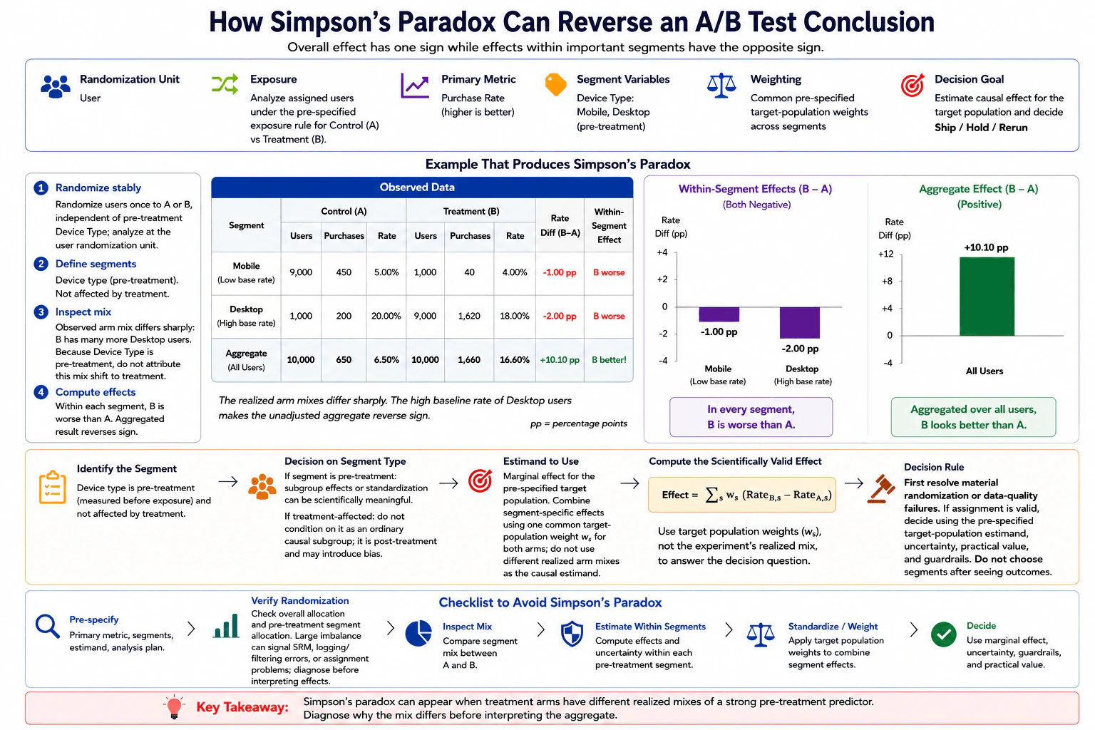
Simpson's paradox appears when an aggregate A/B result has the opposite sign from the effects inside important segments. Here, the randomization unit is the user, Control A is compared with Treatment B, purchase rate is the primary metric, and Device Type is a pre-treatment segment. Treatment B is worse within both Mobile and Desktop, but B contains many more high-converting Desktop users, so its raw overall purchase rate is higher. The key tasks are to diagnose why the arm mix differs, determine whether the segment is pre-treatment, and use the correct pre-specified estimand.

Useful Questions to Ask the Interviewer
  1. Is Device Type measured before treatment exposure, or can treatment affect which segment a user enters?
  2. Was each user assigned once to Control A or Treatment B, independently of pre-treatment Device Type?
  3. What exact pre-specified exposure rule determines which assigned users enter the primary analysis?
  4. Is purchase rate defined as purchases divided by analyzed assigned users under that exposure rule, with higher values considered better?
  5. What target population and segment weights were specified before looking at the outcomes?
  6. Is the extreme Mobile/Desktop allocation imbalance expected from the design, or could it indicate an assignment, filtering, logging, or other data-quality problem?
  7. What uncertainty, practical-value, and guardrail criteria control the final ship, hold, or rerun decision?
How can Simpson's paradox reverse an A/B test conclusion? diagram
How to Explain It in an Interview

Start with the observed reversal. For Mobile users, Control A has a 5.00% purchase rate and Treatment B has 4.00%, so B is worse by 1.00 percentage point. For Desktop users, A has 20.00% and B has 18.00%, so B is worse by 2.00 percentage points. Treatment B therefore underperforms Control A inside both pre-treatment segments.

The raw aggregate says the opposite. Control contains 9,000 Mobile users and 1,000 Desktop users, with 650 purchases among 10,000 users, giving 6.50%. Treatment contains 1,000 Mobile users and 9,000 Desktop users, with 1,660 purchases among 10,000 users, giving 16.60%. The unadjusted aggregate difference is therefore +10.10 percentage points for B.

The reversal happens because Desktop users have a much higher baseline purchase rate than Mobile users, and the realized treatment sample contains far more Desktop users. The aggregate is therefore dominated by different segment weights in the two arms. That arithmetic explains Simpson's paradox, but it does not by itself establish that treatment caused the favorable aggregate result.

Next, determine when the segment is measured. Device Type in this example is pre-treatment: it is defined before exposure and is not caused by treatment. That means subgroup effects and standardization can be scientifically meaningful. If a segment were treatment-affected instead, conditioning on it as an ordinary causal subgroup could introduce post-treatment bias, so I would not apply the same adjustment mechanically.

Then verify the experiment before interpreting any causal effect. Users should be assigned once at the user randomization unit, independently of pre-treatment Device Type. I would check overall treatment allocation, allocation within the pre-treatment segments, assignment logic, exposure construction, logging, filtering, and missing records. The very large conditional allocation imbalance in this example is a strong diagnostic signal. If it comes from broken assignment, sample-ratio mismatch, logging, or differential filtering, I would stop and repair or rerun the experiment before making a causal decision.

If assignment and data quality are valid, define the estimand before choosing weights. For the pre-specified target population, combine segment-specific effects using one common set of target-population weights. The standardized marginal effect is:

Effect = Σ_s w_s × (Rate_B,s - Rate_A,s)

Here, w_s is the pre-specified target-population weight for segment s, and the same w_s is used for both arms. I would not use a different realized segment composition for each arm as the causal weighting scheme because that recreates the misleading aggregate comparison.

Finally, make the decision from the pre-specified estimand rather than from whichever aggregate or subgroup looks favorable after outcomes are visible. Report the effect size with uncertainty, review the pre-specified segment results as supporting evidence, and apply practical-value and guardrail criteria. If the allocation problem invalidates the experiment, rerun or repair it. If assignment is valid, use the target-population marginal effect and the pre-specified decision rule to ship, hold, or rerun.

Technical Approach
  1. Confirm the randomization unit; here it is the user.
  2. Confirm stable assignment to Control A or Treatment B and the pre-specified exposure rule.
  3. Define the primary metric at the same analysis grain; here purchase rate is purchases divided by analyzed assigned users under the exposure rule, and higher is better.
  4. Identify the segment variable and decide whether it is pre-treatment or treatment-affected; Device Type is pre-treatment here.
  5. Compute the treatment effect within Mobile and Desktop before interpreting the aggregate.
  6. Compute the raw aggregate and compare segment proportions across A and B.
  7. Diagnose the extreme realized mix difference by checking overall allocation, within-segment allocation, assignment logic, exposure construction, logging, filtering, and missingness.
  8. If a material randomization or data-quality failure exists, stop causal interpretation and repair or rerun the experiment.
  9. If assignment is valid, use the pre-specified target-population estimand and combine segment-specific effects with one common set of target-population weights: Effect = Σ_s w_s × (Rate_B,s - Rate_A,s).
  10. Report effect size and uncertainty, check pre-specified guardrails and practical value, and make the ship, hold, or rerun decision without choosing segments or weights after seeing outcomes.
Practical Insights

The arithmetic is cheap, but the scientific validation can be expensive. With a few segments, computing subgroup rates and a weighted effect is simple. With many segments, some groups can become small and noisy, uncertainty grows, and multiple-comparison concerns become more important. Standardization also requires defensible target-population weights chosen before outcomes are inspected. The largest risk is not runtime cost. It is making a confident business decision from broken assignment, bad exposure or filtering logic, a treatment-affected segment, or a weighting scheme chosen after seeing results.

Why Interviewers Ask This

This question tests whether a candidate can distinguish a misleading raw aggregate from a scientifically valid causal estimand. It evaluates understanding of randomization, exposure, metric grain, pre-treatment versus treatment-affected variables, allocation diagnostics, Simpson's paradox, standardization, uncertainty, and decision rules. A strong candidate should explain why different segment mixes can reverse the aggregate sign, investigate whether the experiment or data pipeline is broken, and avoid choosing favorable segments or weights after seeing outcomes.

Common interview mistakes

Common mistakes are trusting the raw aggregate because its apparent lift is large; saying treatment caused a change in a pre-treatment segment mix; ignoring an extreme allocation imbalance; analyzing at a different grain from the user randomization unit; using each arm's realized segment proportions as the causal weighting scheme; conditioning on a treatment-affected variable as if it were a normal randomized subgroup; choosing segments or weights after seeing outcomes; reporting only point estimates without uncertainty; and making a ship decision before resolving material assignment or data-quality failures.

Interview tip

Explain the paradox in three steps: show the within-segment effects, show how different segment mixes reverse the raw aggregate, and then state the valid decision rule. Explicitly separate pre-treatment from treatment-affected segments and say that a severe allocation imbalance must be diagnosed before causal interpretation.

Interviewer may ask next
What changes if the segment variable is affected by treatment rather than measured before treatment?

I would not treat it as an ordinary causal subgroup or simply standardize over it. Conditioning on a post-treatment variable can select users based on something caused by treatment and introduce bias. I would keep the primary analysis anchored to randomized assignment and the pre-specified estimand. If the treatment-affected variable is scientifically important, I would analyze it with a causal method appropriate for mediation or post-treatment variables rather than interpreting the conditional A/B difference as a randomized subgroup effect.

What would you do if the Mobile/Desktop imbalance is so large that you suspect the randomization or data pipeline is broken?

I would not make the ship decision from either the raw aggregate or the standardized effect until the problem is understood. I would check overall assignment counts, conditional allocation within the pre-treatment segments, assignment logic, exposure construction, filtering, missing records, and logging. If the imbalance reflects sample-ratio mismatch, assignment failure, or differential data loss, the causal experiment may be invalid and should be repaired or rerun. Only after validating assignment and data integrity would I estimate the pre-specified target-population effect, report uncertainty, and apply the normal guardrail and practical-value decision rule.

57. What is a data pipeline, and how does it move data from sources to analytical or machine learning consumers?Data EngineeringEasy

Question Details

Define a data pipeline and describe ingestion, validation, transformation, storage, orchestration, observability, and delivery. Compare batch and streaming execution, explain how schemas, idempotency, lineage, retries, and data-quality checks protect downstream users, and give one realistic pipeline example for a Data Scientist.

Short Interview Answer (30-60 seconds)

A data pipeline moves data from sources through ingestion, validation, transformation, storage, and delivery. Batch pipelines process chunks on a schedule, while streaming pipelines process events continuously. Contracts, idempotency, quality checks, lineage, monitoring, retries, and backfills help keep downstream analytics and machine learning data reliable.

Detailed Explanation

A data pipeline is a repeatable way to move information from where it is created to where people or computer systems can use it. It can collect information from databases, apps, devices, files, and outside services. Along the way, it checks that the information looks right, handles bad or repeated records, combines and reshapes information, saves it, and makes it available for reports or prediction work. Some pipelines run at set times, while others handle new information as it arrives. Good pipelines also track problems and support safe recovery when something fails.

Useful Questions to Ask the Interviewer
  1. Is the pipeline mainly batch, streaming, or a combination of both?
  2. What are the main source systems and downstream consumers?
  3. What freshness or latency do downstream users need?
  4. How should duplicate, invalid, or late-arriving records be handled?
  5. Are there important retention, access-control, or recovery requirements?
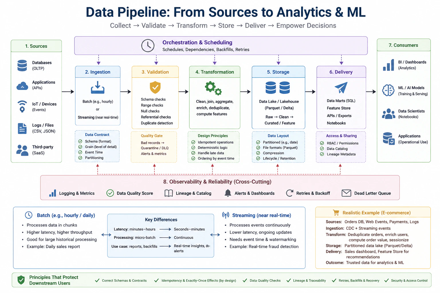
What is a data pipeline, and how does it move data from sources to analytical or machine learning consumers? diagram
How to Explain It in an Interview

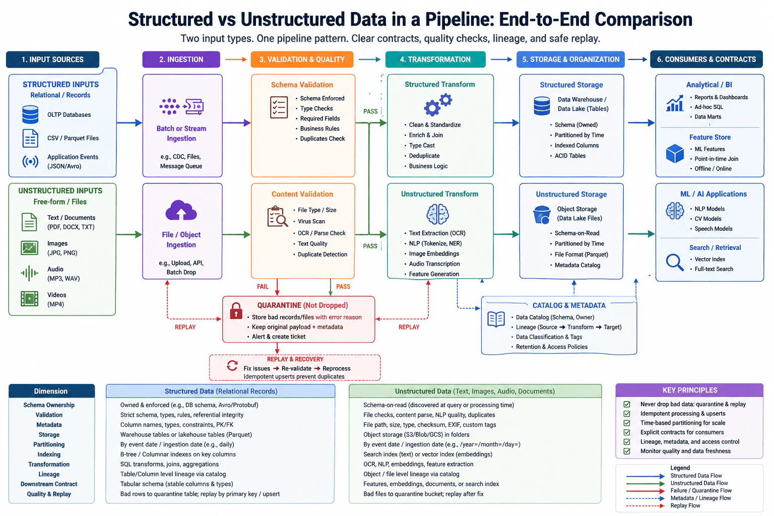
Start with the end-to-end flow shown in the diagram: sources -> ingestion -> validation -> transformation -> storage -> delivery -> consumers. Orchestration and observability are cross-cutting concerns around that flow.

  1. Sources and data contracts Sources can include operational databases, applications or APIs, IoT or device events, logs and files such as CSV or JSON, and third-party services. Before processing, define a data contract. It describes the expected schema, record grain, important event-time fields, and partitioning rules. Grain means what one record represents, such as one order or one event. Schema changes should be managed deliberately so upstream changes do not silently break downstream users.
  1. Ingestion Ingestion collects data from the sources. Batch ingestion processes bounded chunks, such as files or database changes every hour or day. Streaming ingestion receives events continuously or near real time. Change data capture, or CDC, can capture database changes for downstream processing. The ingestion design should retain enough durable information to retry or replay data when recovery or a backfill is needed.
  1. Validation and quality gates Validation checks whether incoming records match the expected contract. The diagram shows schema checks, range checks, null checks, referential checks, and duplicate detection. Bad records can be quarantined or sent to a dead-letter queue instead of entering trusted datasets. Quality metrics and alerts help detect situations where the pipeline technically runs but produces incorrect or incomplete data.
  1. Transformation Transformation can clean, join, aggregate, enrich, deduplicate, and compute features. The logic should be deterministic and idempotent. Idempotent means that retrying the same logical input does not create duplicate business effects. For streaming data, event time is when the event happened, while processing time is when the pipeline handles it. Watermarks help decide how long to wait for late events. Ordering should be defined only where needed; a distributed pipeline should not assume global ordering of all events.
  1. Storage Validated and transformed data can be stored in a data lake or lakehouse, warehouse, data mart, or feature store depending on the consumer. A common organization is raw -> clean -> curated or feature data. The diagram uses Parquet or Delta as representative analytical storage formats. Partitioning, for example by date when appropriate, can reduce the amount of data read. Retention and lifecycle policies control how long data remains available.
  1. Delivery and consumers Trusted data is delivered to BI dashboards, SQL analysis, notebooks, data scientists, machine learning training or serving, APIs, exports, and operational applications. Data marts can expose analysis-ready SQL data, while a feature store can expose reusable machine learning features. Access controls such as role-based permissions protect sensitive datasets, and catalog or lineage metadata helps consumers discover and understand data.
  1. Orchestration Orchestration manages schedules, task dependencies, retries, and backfills. For example, transformation should not begin until required ingestion and validation steps are ready. A backfill reprocesses historical data after a bug, missing input, or logic change. Backfills should use deterministic and idempotent logic so reprocessing does not silently duplicate or corrupt existing results.
  1. Observability, lineage, and recovery Observability includes logging, metrics, data-quality measurements, lineage, alerts, and dashboards. Lineage records how data moves from sources through transformations to consumers, which helps with debugging and impact analysis. Retries with backoff handle transient failures, and a dead-letter queue can isolate records that repeatedly fail validation or processing. Streaming systems may use checkpoints to resume progress after failures. These mechanisms do not automatically guarantee exactly-once business outcomes; safe outcomes still depend on the application logic and destination writes being idempotent or transactional where required.

Batch versus streaming Batch processing handles data in bounded chunks and is commonly used for reports, large historical jobs, and backfills. It usually has higher latency but is simpler to operate. Streaming processes events continuously and supports lower-latency dashboards, alerts, and model inputs. It requires more care with state, checkpoints, event time, watermarks, duplicates, ordering, and late data. Micro-batching is a middle ground that processes small batches frequently. Choose the simplest execution model that meets the required freshness and correctness.

Realistic Data Scientist example Consider an e-commerce pipeline like the one in the diagram. Sources include an orders database, web events, payments, and logs. Order changes can arrive through CDC, while web activity can arrive as streaming events. Validation applies schema and quality checks, and bad records are quarantined. Transformation deduplicates orders, enriches events with user information, computes order value, and sessionizes activity. The output is stored in a partitioned analytical lake or lakehouse using formats such as Parquet or Delta. Curated data feeds sales dashboards, while reusable features can feed a feature store for recommendation models. Logging, quality checks, lineage, retries, backfills, retention policies, and access controls protect downstream users.

Technical Approach
  1. Identify source systems, downstream consumers, data grain, and freshness requirements.
  2. Define the data contract, including schema, event-time fields, and partitioning rules.
  3. Choose batch, micro-batch, streaming, or a combination based on latency needs.
  4. Ingest data with enough durability for retries, replay, or backfills.
  5. Validate schema and data-quality rules; quarantine invalid records.
  6. Transform with deterministic, idempotent logic and explicit handling of duplicates and late data.
  7. Store raw, clean, curated, or feature data with suitable formats, partitioning, retention, and access controls.
  8. Deliver trusted data to analytics, notebooks, feature stores, ML systems, APIs, or applications.
  9. Orchestrate dependencies, retries, and backfills.
  10. Monitor logs, metrics, quality, lineage, alerts, and recovery behavior.
Practical Insights

The main costs are data volume, processing frequency, storage, and operations. Batch pipelines usually run compute only during scheduled jobs and are simpler to operate, but users wait longer for fresh data. Streaming keeps processing active and often needs state, checkpoints, watermark handling, and more monitoring, so operational complexity is higher. Partitioning and columnar formats can reduce analytical scan cost, while retention policies limit storage growth. Quality checks, lineage, idempotency, retries, and backfill support add engineering work but reduce the risk and cost of incorrect or unrecoverable downstream data.

Why Interviewers Ask This

Interviewers want to see whether the candidate understands a data pipeline as an end-to-end production system rather than only a transformation script. They evaluate whether the candidate can explain ingestion, validation, transformation, storage, orchestration, observability, delivery, batch versus streaming execution, and the reliability practices that protect analytical and machine learning consumers.

Common interview mistakes

Common mistakes include describing a pipeline as only ETL code; skipping the source and destination contracts; ignoring record grain; assuming retries are automatically safe; claiming a streaming engine alone guarantees exactly-once business outcomes; confusing event time with processing time; assuming global event ordering; ignoring duplicates or late data; allowing bad records to silently enter trusted datasets; monitoring only infrastructure instead of data quality; omitting lineage; running unsafe backfills; and forgetting retention or access control. Another mistake is choosing streaming simply because it sounds more advanced when batch processing already meets the required freshness.

Interview tip

Explain the pipeline from left to right: sources, ingestion, validation, transformation, storage, delivery, and consumers. Then explain the cross-cutting concerns: orchestration, observability, contracts, quality, idempotency, lineage, retries, backfills, retention, and access control. Finish by comparing batch with streaming and giving the e-commerce example.

Interviewer may ask next
How would you choose between a batch pipeline and a streaming pipeline?

Start with the freshness requirement. If data can be minutes or hours old, scheduled batch processing is usually simpler to operate. If users need updates within seconds or a few minutes, streaming may be justified. Streaming also requires explicit handling of state, checkpoints, event time, watermarks, duplicates, ordering, and late events. Micro-batching can be a useful middle ground. Choose the simplest model that meets both latency and correctness requirements.

How do you make retries and backfills safe without creating duplicate data?

Use idempotent processing so replaying the same logical input produces the same intended final state rather than another copy. Keep stable record or event identifiers, preserve the intended grain, deduplicate when necessary, and use deterministic replacement, merge, or transactional destination writes when the storage system supports them. Track processing progress, validate backfill output, and keep lineage so affected downstream datasets are known. Transport-level delivery guarantees alone are not enough to guarantee exactly-once business outcomes.

58. What is data modeling, and why does grain matter?Data EngineeringEasy

Question Details

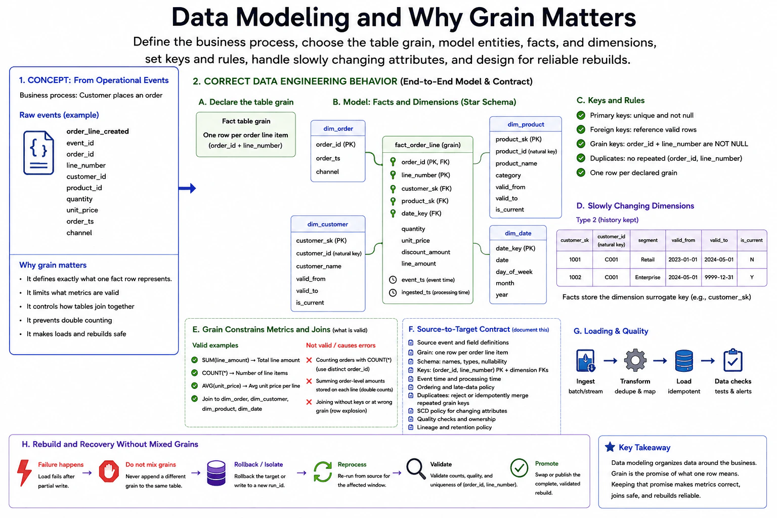
A team is designing analytical tables from operational events. Define the business process, table grain, entities, facts, dimensions, primary and foreign keys, null and duplicate rules, and slowly changing attributes. Explain how the declared grain constrains valid metrics and joins, what source-to-target contract should be documented, and how a rebuild or failed load can recover without producing mixed grains.

Short Interview Answer (30-60 seconds)

Data modeling defines how business data is represented and related. Grain defines exactly what one fact row means. Once grain is declared, facts, keys, joins, metrics, duplicate rules, historical dimensions, and recovery must stay consistent with that level so analytics remain correct and rebuilds do not create mixed-grain data.

Detailed Explanation

The first decision is to define what each row means before building the table. Imagine a store wants to analyze customer orders. The team must decide whether one row represents a whole order, one item inside an order, or another business activity. That choice controls which numbers can be added, which records can be connected, how repeated records are handled, and how changes are remembered over time. If different row meanings are mixed in the same table, reports can count activity more than once, connect records incorrectly, or produce unreliable results after a failed rebuild.

Useful Questions to Ask the Interviewer
  1. What business process should the analytical table represent?
  2. What should exactly one fact-table row represent?
  3. Which measures must be calculated from this table?
  4. Which descriptive attributes need historical tracking when they change?
  5. What uniquely identifies a source event and the declared business grain?
  6. How should duplicate, late, or replayed source records be handled?
  7. Should failed loads be rebuilt for the full table or only an affected time window or partition?
What is data modeling, and why does grain matter? diagram
How to Explain It in an Interview

Start with the practical decision: define the business process and declare the grain before choosing columns. The business process in this example is a customer placing an order. The operational source produces an order_line_created event, and the analytical destination uses a fact-table grain of one row per order line item. The business grain key is (order_id, line_number).

The main business entities are orders, order lines, customers, products, and dates. The source event can carry event_id, order_id, line_number, customer_id, product_id, quantity, unit_price, order_ts, and channel. The destination is a dimensional analytical model with a central fact_order_line table connected to descriptive dimensions.

The central fact table is fact_order_line. Its order_id and line_number form the composite primary key representing the declared grain. order_id is also a foreign key to dim_order. The fact contains additional foreign keys such as customer_sk, product_sk, and date_key. Measures such as quantity, unit_price, discount_amount, and line_amount belong in the fact because they describe the order-line row.

Dimensions provide descriptive context. dim_order contains order-level attributes such as order_ts and channel. dim_date provides calendar attributes. dim_customer and dim_product use surrogate keys. A surrogate key is an internal identifier for one specific dimension row and is different from a durable business identifier such as customer_id or product_id.

Slowly changing attributes need an explicit history policy. With a Type 2 slowly changing dimension, a changed attribute creates a new dimension row instead of overwriting the old row. For example, customer C001 can have surrogate key 1001 while the customer is in the Retail segment and surrogate key 1002 after changing to Enterprise. Fields such as valid_from, valid_to, and is_current identify when each version applies. Facts store the surrogate key of the dimension version that applies to the fact, preserving historical meaning.

Primary-key, foreign-key, null, and duplicate rules must agree with the declared grain. The grain keys order_id and line_number are not null, and the target cannot contain repeated (order_id, line_number) combinations. Foreign keys should reference valid dimension rows. Duplicate or replayed input should be rejected or idempotently merged so reprocessing the same business record does not create another fact row.

Grain also constrains metrics. At one row per order line, SUM(line_amount) gives total line amount, COUNT(*) gives the number of line items, and AVG(unit_price) gives the average unit price per fact row. Counting orders requires COUNT(DISTINCT order_id) because one order can contain several lines. An order-level amount copied onto every order line must not be summed directly because it would be double counted. Joining tables using incompatible keys or grains can multiply rows and corrupt metrics.

The source-to-target contract should document the source event and field definitions; declared grain; column names, types, and nullability; the (order_id, line_number) primary key and dimension foreign keys; event-time and processing-time meaning; ordering and late-data policy; duplicate and replay behavior; slowly changing dimension policy; quality checks and ownership; lineage; and retention policy. These rules make the transformation from operational events to analytical tables explicit and testable.

Event time and processing time should be distinguished. Event time is when the business event occurred, represented here by the event or order timestamp. Processing time is when the pipeline handled the record. The contract should state how ordering and late-arriving records are treated rather than assuming records always arrive in business-event order.

The loading flow is ingest, transform, load, and validate. Transformation includes mapping source fields to the target model and applying duplicate rules. The target load should be idempotent, meaning rerunning the same input produces the same final business result instead of additional rows. Data checks should verify the declared grain, uniqueness of (order_id, line_number), required fields, valid foreign keys, and important measure rules.

Recovery must not combine an uncertain partial result with a new rebuild. If a load fails after a partial write, isolate or roll back the affected target state. Reprocess the affected source scope using the same declared grain and duplicate rules. Then validate row counts, quality rules, and uniqueness of (order_id, line_number). Only after the rebuilt result is complete should it be promoted or swapped into the analytical target. This prevents partial old data and newly rebuilt data from becoming mixed.

The key idea is simple: grain is the promise of what one row means. Once that promise is declared, entities, facts, dimensions, keys, metrics, joins, duplicate handling, historical attributes, validation, and recovery must all preserve it.

Technical Approach
  1. Define the business process being analyzed.
  2. Identify the important entities, such as orders, order lines, customers, products, and dates.
  3. Declare the fact-table grain in one sentence, such as one row per order line item.
  4. Define the grain key, here (order_id, line_number).
  5. Separate measurable facts from descriptive dimensions.
  6. Define primary keys, surrogate dimension keys, foreign keys, null rules, and duplicate rules.
  7. Decide which changing dimension attributes require Type 2 history.
  8. Document the source-to-target contract, including schema, time semantics, ordering, late-data handling, replay behavior, quality ownership, lineage, and retention.
  9. Check every proposed metric and join against the declared grain to prevent double counting or row multiplication.
  10. Make target writes idempotent and validate grain-key uniqueness and foreign-key validity.
  11. For failures or backfills, rebuild an isolated affected scope, validate it completely, and promote it only after it passes checks.
Practical Insights

The main cost is data and operational complexity rather than algorithmic complexity. A finer grain, such as one row per order line instead of one row per order, creates more rows and therefore increases storage, transformation, validation, and maintenance work. Type 2 dimensions also keep historical versions, which increases dimension size. Correct grain reduces downstream confusion because metrics and joins have predictable meaning. Safe rebuilds may require temporary storage for an isolated replacement dataset, but they reduce the risk of duplicates, partial results, and mixed-grain tables.

Why Interviewers Ask This

Interviewers want to see whether the candidate can turn operational events into trustworthy analytical tables. They are testing whether the candidate understands that grain is a design contract, not just a description. A strong answer connects grain to business entities, facts, dimensions, primary and foreign keys, null and duplicate rules, slowly changing attributes, valid metrics, safe joins, source-to-target contracts, quality checks, lineage, and failure recovery.

Common interview mistakes

Common mistakes are choosing columns before declaring the grain; mixing order-level and order-line-level facts in one table; using a natural customer identifier as the unique row key of a Type 2 dimension; omitting required foreign keys; allowing null or repeated grain keys; copying an order-level amount onto every order line and then summing it; counting fact rows when the required metric is distinct orders; joining tables at incompatible grains and multiplying rows; overwriting dimension history; treating arrival order as guaranteed event order; assuming retries are safe without idempotency; and rebuilding directly into a partially written target so old and new data become mixed.

Interview tip

State the business process and grain first and keep returning to them. A strong answer can use one example throughout: one row per order line. Then show how that decision determines the primary key, foreign keys, measures, dimensions, valid metrics, duplicate rules, Type 2 history, source-to-target contract, quality checks, and safe recovery.

Interviewer may ask next
What happens if a table contains both order-level and order-line-level measures?

The table contains mixed grains, so metrics become ambiguous and can be double counted. For example, if an order total is repeated on every order line, summing that field multiplies the order amount by the number of lines. The safer design is to keep each fact table at one declared grain or deliberately transform a higher-level value into a valid line-level allocation using an explicit business rule.

How would you safely rebuild this fact table after a partial failed load?

Do not append a new rebuild on top of an uncertain partial result. Isolate or roll back the affected target scope, rerun the source data for that scope with the same one-row-per-order-line grain and idempotent duplicate rules, and validate counts, required fields, foreign keys, and uniqueness of (order_id, line_number). Promote or replace the affected target only after the complete rebuilt result passes validation.

59. How do structured and unstructured data differ in a pipeline?Data EngineeringEasy

Question Details

Compare relational records with free-form text, images, audio, or documents as pipeline inputs. For each, define schema ownership, validation, metadata, storage, partitioning, indexing, transformation, lineage, and downstream analytical or feature contracts. Include how malformed items are quarantined and replayed rather than silently dropped.

Short Interview Answer (30-60 seconds)

Structured data has a known record shape and stronger upfront schema checks. Unstructured data needs file-level validation, richer metadata, content extraction, and often full-text or vector indexing. Both paths still require explicit contracts, lineage, quality checks, partitioning, and quarantine plus replay for failures.

Detailed Explanation

This question asks how a data pipeline should handle two kinds of input. One kind arrives in predictable records with known values. The other can be free-form text, documents, pictures, sound, or video whose useful information must be extracted. You should explain who defines what valid input looks like, how bad items are detected, what metadata is kept, where data is stored, how it is organized and searched, what processing prepares it for users, how its history is tracked, and how failed items are saved and tried again instead of being lost.

Useful Questions to Ask the Interviewer
  1. Should I discuss both batch and streaming ingestion, or focus on the common pipeline design?
  2. Can I assume the structured records have an owned schema before ingestion?
  3. Are the unstructured outputs mainly intended for analytics, search, machine learning features, or all three?
  4. Should the quarantine path retain the complete original payload so failed items can be replayed safely?
How do structured and unstructured data differ in a pipeline? diagram
How to Explain It in an Interview

Start with the practical difference. Structured data has a predictable record shape. Unstructured data contains content whose useful structure usually has to be discovered or extracted during processing.

For structured inputs, examples include relational database records, CSV or Parquet files, and typed application events. The source or data-owning team should own an explicit schema contract. The contract defines fields, data types, required values, keys, allowed ranges, and compatibility expectations when the schema evolves.

During validation, the pipeline can perform type checks, required-field checks, business-rule checks, uniqueness or duplicate checks, and referential checks when relationships between records require them. Invalid records should not be silently discarded.

Structured metadata commonly includes the dataset name, columns, data types, key information, schema version, source, owner, ingestion information, and lineage. After cleaning and transformation, trusted structured data is commonly stored in warehouse or lakehouse tables. It can be partitioned by a useful time field when that matches the query pattern and data volume. Depending on the storage system, frequently filtered fields can also use indexes, clustering, or sort keys.

Structured transformations commonly include cleaning, standardization, type casting, deduplication, joins, enrichment, aggregation, and business logic. Writes used during retries or backfills should be idempotent where practical. Idempotent means repeating the same logical operation does not create an unintended second result.

The downstream structured-data contract should state the output table schema and its grain. Grain means what one row represents, for example one user per day. The contract should also describe important semantics, freshness expectations, and compatibility rules so reports, ad-hoc SQL, data marts, feature stores, and machine-learning consumers do not silently receive a different meaning.

For unstructured inputs, examples include free-form text, documents such as PDF or DOCX files, images, audio, and video. These items usually arrive as files or objects through uploads, APIs, batch drops, or similar ingestion paths. The first contract is therefore often about the object and its metadata rather than a fixed set of business columns.

Unstructured validation can check file type, size, readability, checksum, duplicate identity, and content-specific validity. Documents may be tested for successful parsing or OCR. Images, audio, or video may be checked to confirm they can be decoded. Security-oriented checks such as malware scanning can also be appropriate for externally supplied files.

Metadata is especially important for unstructured data. Useful fields can include an object ID, original filename, media type, size, checksum, source, owner, timestamps, processing status, and processing version. The original payload is commonly retained in object storage so it can be audited, reprocessed, or replayed later.

Raw unstructured objects should normally remain in their native file formats. Derived structured outputs, such as extracted text, document chunks, transcripts, or feature tables, can be stored in formats such as Parquet when that is useful for analytical processing. Object collections can be organized or partitioned by ingestion date or another stable operational attribute when that matches retention and access patterns.

Indexing differs between the two paths. Structured data usually relies on indexes, clustering, sorting, or partition pruning over known fields. Extracted text can use a full-text search index. Content intended for semantic retrieval can be converted into embeddings and stored in a vector index. These indexes are derived serving structures; the original object and metadata should remain available for lineage and replay.

Unstructured transformations depend on the media. Documents may require parsing or OCR. Text may require tokenization, entity extraction, or other NLP processing. Audio may require transcription. Images may produce embeddings or other features. These steps often turn free-form inputs into structured artifacts that downstream systems can consume.

The downstream contract for unstructured data should define those derived artifacts. A document pipeline might publish one record per document or one record per chunk with document_id and chunk_id as the grain. A feature pipeline might publish one embedding per object or chunk. The contract should state the meaning, identifiers, version, and freshness expectations of those outputs.

Consumers also differ. Structured outputs commonly feed BI reports, dashboards, ad-hoc SQL, data marts, and feature stores. Unstructured outputs commonly feed search and retrieval, NLP applications, computer-vision models, speech models, machine-learning training, and data-science workflows.

Lineage is required for both. Structured lineage should connect source records or tables through transformations to destination tables or features. Unstructured lineage should connect the original file or object to extracted text, chunks, transcripts, embeddings, or other derived artifacts. Recording schema and transformation versions helps explain why the same source might produce a different derived result after the processing logic changes.

Failure handling should also follow the same reliability rule for both paths. When validation fails, place the malformed record or file in quarantine rather than dropping it. Store the original payload, identifying metadata, failure reason, and processing or schema version. Alert or monitor the failure so it is visible.

After the data or processing problem is corrected, revalidate and replay the quarantined item. Replay should use idempotent processing, deduplication, or stable-key upserts so repeating an item does not create unintended duplicates. The same mechanism supports historical backfills when transformation logic or downstream contracts change.

Retention and access-control policies apply to both raw and derived data. This is especially important for documents, audio, images, or other files that may contain sensitive information.

The main tradeoff is that structured data gives stronger validation earlier and is usually easier to query directly, but schema evolution must be managed carefully. Unstructured data accepts richer and more varied inputs, but it needs more metadata, extraction work, storage, specialized indexing, and operational controls before downstream consumers can use it reliably.

Technical Approach
  1. Classify the input as a structured record or an unstructured file or object and identify the owner of its input contract.
  2. Ingest through the appropriate path, such as batch, CDC, streaming, file upload, API, or batch drop.
  3. Validate structured records with schema, type, required-field, business-rule, uniqueness, duplicate, and referential checks where relevant.
  4. Validate unstructured items with file type, size, checksum, readability, parsing or decoding, duplicate, and content-quality checks where relevant.
  5. Capture metadata, source, owner, identifiers, schema or processing version, and lineage before downstream transformation.
  6. Quarantine failed records or files with the original payload and failure reason instead of silently dropping them.
  7. Transform valid structured data with cleaning, standardization, joins, enrichment, type casting, deduplication, aggregation, or other business logic.
  8. Transform valid unstructured data with parsing, OCR, NLP, transcription, embedding generation, or media-specific feature extraction.
  9. Store structured outputs as curated warehouse or lakehouse tables and retain raw unstructured payloads in object storage; store derived unstructured artifacts separately as needed.
  10. Choose partitioning and indexing according to access patterns: time-based partitioning when appropriate, field-oriented indexing for structured data, and full-text or vector indexes for extracted unstructured content when required.
  11. Publish explicit analytical or feature contracts that define schema, grain, semantics, identifiers, versions, and freshness expectations.
  12. After correcting a failure, revalidate and replay quarantined items with idempotent writes, stable keys, upserts, or deduplication so retries and backfills do not create unintended duplicates.
Practical Insights

Structured pipelines are usually simpler to validate because the fields and types are already known. Their main maintenance cost is controlling schema changes and keeping downstream contracts compatible. Unstructured pipelines often need more storage because the original files are retained, and they add processing cost for OCR, NLP, transcription, embeddings, or other feature extraction. Full-text and vector indexes add more storage and compute. Both designs also need metadata catalogs, lineage, monitoring, quarantine storage, replay logic, retention policies, access controls, and backfill support. Partitioning can reduce how much data must be scanned, but excessive partitions or many small files can increase operational overhead.

Why Interviewers Ask This

Interviewers want to know whether you understand how the data type changes validation, metadata, storage, indexing, transformation, lineage, and downstream contracts. They also want to see operational judgment: malformed records or files should be quarantined with their original payload and failure reason, then safely replayed instead of disappearing.

Common interview mistakes

A common mistake is saying only that structured data has rows and columns while unstructured data does not. That ignores the pipeline implications. Other mistakes include treating unstructured data as if it needs no contract, failing to retain rich object metadata, assuming raw unstructured files should be converted directly into tables, confusing a derived search or vector index with the source of truth, using the same validation or indexing strategy for both data types, omitting downstream grain and contract definitions, ignoring schema or processing-version changes, and silently dropping malformed inputs. Another serious mistake is replaying failures without idempotency or deduplication, which can create duplicate outputs.

Interview tip

Compare the two paths using the same stages: source and contract, ingestion, validation, metadata, transformation, storage and partitioning, indexing, lineage, downstream consumers, and failure recovery. Emphasize that the implementation differs by data type, but the reliability rule is shared: keep the original data, make contracts explicit, quarantine failures, and replay them safely.

Interviewer may ask next
How would you handle a malformed document or structured record without losing data?

I would route the failed item to a quarantine location instead of dropping it. I would retain the original payload, stable identifier, source metadata, schema or processing version, and an explicit error reason. The failure should be visible through monitoring or alerts. After correcting the data or processing logic, I would revalidate and replay the item. The destination write should use a stable key, upsert, or deduplication rule so replay is idempotent and does not create unintended duplicates.

Why might an unstructured-data pipeline use both object storage and a full-text or vector index?

They solve different problems. Object storage keeps the original document, image, audio, video, or other payload together with durable metadata for retention, lineage, audit, reprocessing, and recovery. A full-text index stores analyzed text for lexical retrieval, while a vector index stores embeddings for similarity or semantic retrieval. Those indexes are derived serving structures and can be rebuilt from retained source data and transformation metadata, so they should not be the only copy of the content.

60. When would you choose a star schema rather than a snowflake schema?Data EngineeringEasy

Question Details

A warehouse must support repeatable business metrics over facts joined to descriptive dimensions. Compare denormalized star dimensions with normalized snowflake dimensions in terms of grain, key integrity, storage, update anomalies, query simplicity, performance, governance, and slowly changing history. Define how source changes are loaded and how a failed dimension or fact publish is recovered atomically.

Short Interview Answer (30-60 seconds)

I choose a star schema when simple, repeatable analytics and fewer joins matter more than minimizing repeated dimension data. It is easier for analysts and often faster for reporting. I choose a snowflake when normalization, reduced repetition, or large reusable hierarchies justify the additional tables, keys, and joins.

Detailed Explanation

The question asks how to organize business data so people can calculate the same numbers repeatedly and get consistent results. One design keeps descriptive information together, which makes reports easier to understand and usually needs fewer connections. The other breaks that information into more related pieces, which can reduce repetition but makes reporting more complex. You also need to explain how changed information is stored over time, how new records are checked before users can see them, and what happens if only part of an update succeeds so nobody sees an incomplete release.

Useful Questions to Ask the Interviewer
  1. Are simple analyst queries and reporting performance more important than minimizing repeated descriptive data?
  2. How large and frequently changing are the dimensions and their hierarchies?
  3. Do historical reports need to preserve old dimension values with SCD Type 2?
  4. What warehouse or storage system is used, and which atomic publish operations does it support?
When would you choose a star schema rather than a snowflake schema? diagram
How to Explain It in an Interview

I would start with the fact grain. If the grain is one row per order line, every fact row must continue to represent exactly one order line in either design.

In a star schema, descriptive dimensions such as customer, product, date, and store connect directly to the fact table. The dimensions are denormalized, so descriptive values can repeat. That can use more storage and can create more update-anomaly risk, but it gives fewer joins, simpler SQL, easier analyst use, and often better analytical query performance.

In a snowflake schema, a dimension is normalized into additional related tables. For example, product can be separated into product, subcategory, and category, or store can reference region. This reduces repeated dimension data and can reduce update anomalies, but it creates more foreign-key relationships, more joins, more SQL complexity, and more objects to govern. Queries may therefore cost more depending on the warehouse and workload.

Key integrity matters in both designs. Facts should reference valid dimension keys. Stable surrogate keys are useful for warehouse relationships because source business keys can change or be reused.

For slowly changing history, I would use SCD Type 2 when the business must preserve old dimension values. A changed dimension member receives a new version rather than overwriting the old row. Fields such as effective_start, effective_end, and is_current identify the valid period. Facts should point to the dimension version that was valid for the relevant business event.

For loading, source changes can arrive from systems such as CRM, ERP, or e-commerce applications. They first go to a raw or staging area through batch or streaming ingestion. In staging, clean and standardize records, deduplicate them deterministically, and use event_time when ordering or historical matching requires it. Then build or update dimensions, resolve dimension keys, and load facts at the defined grain.

Before publication, run quality checks such as schema validation, row-count checks, null checks, range checks, uniqueness checks where required, and referential-integrity checks. The exact checks depend on the warehouse contract.

For publication, keep the new data unpublished until dimensions and facts both pass validation. Then use one atomic publish operation supported by the platform, such as a partition swap, table-pointer swap, rename, or transaction where supported. Consumers such as BI dashboards, reports, and exports should see either the old complete release or the new complete release, never a partial one.

If a dimension or fact step fails before publish, do not swap or commit. Leave the current published data unchanged, alert and stop the failed run, correct the issue, rebuild or reuse deterministic staging data, rerun validation, and publish again. Idempotent keys and deterministic transformations let retries and backfills reproduce the same result instead of creating duplicate business records.

Technical Approach
  1. Define the fact-table grain, such as one row per order line.
  2. Identify descriptive dimensions and their warehouse keys.
  3. Prefer a star schema when fewer joins, simpler SQL, analyst usability, and repeatable reporting are the main goals.
  4. Prefer a snowflake when reducing repeated dimension attributes, normalizing large hierarchies, or reducing update anomalies is worth the extra joins and governance objects.
  5. Define SCD behavior for attributes whose history must be preserved.
  6. Ingest source changes into raw or staging storage using the required batch or streaming process.
  7. Clean, standardize, and deterministically deduplicate staged records.
  8. Build or update dimensions first and resolve stable dimension keys.
  9. Load facts at the unchanged business grain.
  10. Run schema, count, null, range, uniqueness, and referential-integrity checks as required by the data contract.
  11. Publish the validated dimensions and facts through one warehouse-supported atomic operation.
  12. If the run fails before publish, keep the previous published release unchanged, correct the issue, rerun idempotently, validate again, and republish.
Practical Insights

A star schema normally has fewer tables and joins, so queries are easier to write and often require less join work. The cost is that descriptive values can repeat, so dimensions may use more storage and some changes can touch repeated data. A snowflake can reduce repeated dimension values and some update anomalies, but it adds tables, keys, joins, lineage relationships, and governance work. SCD Type 2 also uses extra storage because old versions are retained. Staging, validation, and atomic publishing add temporary storage and operational steps, but they prevent incomplete releases from reaching users.

Why Interviewers Ask This

Interviewers want to know whether you understand the practical tradeoff between denormalized and normalized dimensional models. They are testing whether you can protect fact grain and key integrity, reason about storage, update anomalies, query complexity, performance, governance, slowly changing history, and design a safe load-and-recovery process that avoids exposing partially published warehouse data.

Common interview mistakes

Common mistakes are changing the fact grain during modeling, treating source business keys as permanently stable, saying a star schema is always faster, saying a snowflake always uses less total storage, normalizing dimensions without considering analyst complexity, overwriting historical attributes when SCD Type 2 is required, loading facts before their dimension keys resolve, skipping referential-integrity checks, assuming transport retries provide exactly-once business results, and publishing dimensions and facts separately so consumers can observe a partial release. Another mistake is assuming every warehouse supports the same atomic swap operation.

Interview tip

Start with the decision and tradeoff: use a star schema for simpler, repeatable analytics with fewer joins; use a snowflake when normalization benefits justify extra complexity. Then cover grain, keys, SCD history, quality checks, and atomic recovery. Qualify performance statements with words such as "often" or "may" because the actual result depends on the warehouse and workload.

Interviewer may ask next
How would you preserve customer history if a customer's descriptive attributes change?

Use SCD Type 2. Keep the previous customer row with its original surrogate key and historical validity period, then insert a new customer version with a new surrogate key. Fields such as effective_start, effective_end, and is_current identify which version was valid at each time. New facts should resolve to the version valid for their business event, while old facts continue referencing the historical version.

What should happen if the dimension build succeeds but the fact load fails before publication?

Do not publish the new release. Keep the current published warehouse unchanged and leave the new dimension and fact data in staging or another unpublished location. Correct the failure, rerun the deterministic or idempotent processing, rebuild or reuse staging data as appropriate, rerun all required checks, and only then publish both parts through one warehouse-supported atomic operation so consumers never see a partial state.

More questions load as you scroll

Disclaimer: This interview guide is for educational and informational purposes only. It is designed to help readers prepare, but it does not guarantee any interview result, hiring decision, offer, or outcome. Interview questions, hiring criteria, and preferred answers can vary by employer, interviewer, industry, location, and time. The examples and explanations reflect the authors' research and judgment, are provided without warranties of any kind, and should not be treated as the only correct approach. Diagrams are simplified illustrations intended to highlight the main components and their interactions; actual systems and implementations may be more complex. Alternative approaches may be equally valid or better suited to a particular question, context, or interviewer. To the fullest extent permitted by applicable law, the author, contributors, and publisher are not liable for decisions made, actions taken, or losses incurred based on this guide.

Content Accuracy and Verification: To the fullest extent permitted by applicable law, we do not represent or warrant that interview guides, questions, answers, examples, or diagrams are accurate, complete, current, error-free, or suitable for any particular purpose. You are responsible for independently reviewing and verifying the information before relying on it.