This interview guide is for educational and informational purposes only. It is designed to help readers prepare, but it does not guarantee any interview result, hiring decision, offer, or outcome. Interview questions, hiring criteria, and preferred answers can vary by employer, interviewer, industry, location, and time. All answers, examples, and explanations in this guide are suggested examples for interview preparation, not definitive answers or instructions for professional practice. They are based on research and judgment, are provided without warranties of any kind, and should be adapted to the question, role, and applicable laws and professional requirements. Diagrams are simplified illustrations intended to highlight the main concepts and their relationships; actual situations, systems, and practices may be more complex. Alternative approaches may be equally valid or better suited to a particular question, context, or interviewer. To the fullest extent permitted by applicable law, the contributors and publisher are not liable for decisions made, actions taken, or losses incurred based on this guide.
State Laws and Professional Responsibilities
Laws and requirements governing an occupation vary by state and jurisdiction. You are responsible for checking the current laws, licensing requirements, and scope-of-practice rules that apply to your location and role, and for ensuring that your answers and actions comply with them. Adapt examples in this guide to those requirements. This guide is not legal advice.
Identity, Image, and Privacy Notice
To respect individual privacy, some names, profile photographs, avatars, biographical details, and other identifying information displayed in this guide may be replaced with pseudonyms, licensed stock images, illustrative avatars, composite images, or representative descriptions. Unless a person is expressly identified as an actual contributor, a displayed name, image, or profile should not be understood as depicting or identifying a specific candidate, interviewer, employee, or other real individual. These representations are provided for editorial and illustrative purposes only and do not imply endorsement, employment, participation, or affiliation with this guide or any company mentioned in it. Any resemblance to an actual person is coincidental.
Company Notice
This guide is an independent educational resource and is not affiliated with, endorsed by, sponsored by, or approved by the company named in this guide. Company names identify reported interview experiences or the employer context of clearly labeled original practice exercises. Interview practices can change without notice, and inclusion of company-specific content does not mean these questions are official, complete, or guaranteed to be asked. To the fullest extent permitted by law, the author, contributors, and publisher are not responsible for outcomes related to use of this material.
Content Accuracy and Verification
To the fullest extent permitted by applicable law, we do not represent or warrant that interview guides, questions, answers, examples, or diagrams are accurate, complete, current, error-free, or suitable for any particular purpose. You are responsible for independently reviewing and verifying the information before relying on it.
Questions or comments?
Contact us for general questions, or share feedback, technical corrections, and comments with the community.
71. Summarize monthly transactions by country.Sql And DatabaseMedium
i Question Details
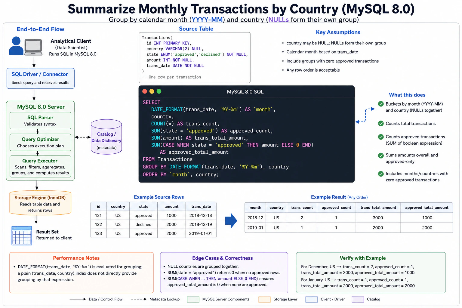
Use MySQL 8.0. Table Transactions(id INT PRIMARY KEY, country VARCHAR(2) NULL, state ENUM('approved','declined') NOT NULL, amount INT NOT NULL, trans_date DATE NOT NULL) has one row per transaction; country may be null and null countries form their own group. Group by calendar month formatted YYYY-MM and country. Return columns month, country, trans_count, approved_count, trans_total_amount, and approved_total_amount; include groups with zero approved transactions and allow any row order. Example rows (121,'US','approved',1000,'2018-12-18'),(122,'US','declined',2000,'2018-12-19'),(123,'US','approved',2000,'2019-01-01') produce December US counts 2,1 and totals 3000,1000, plus January US counts 1,1 and totals 2000,2000.
Short Interview Answer (30-60 seconds)
Group the Transactions table by YYYY-MM and country. Count every row, conditionally count approved rows, sum every amount, and conditionally sum approved amounts. Keep declined rows in the input so groups with zero approvals still appear, and let NULL countries form one group.
Each row in the table is one transaction. The task is to turn those individual rows into a monthly summary for each country. For every month and country, we need the total number of transactions, the number that were approved, the total amount, and the approved amount. Missing countries must still appear as their own group. A group must also remain when it has transactions but none are approved. The three supplied rows therefore create one US result for December 2018 and one US result for January 2019.
Useful Questions to Ask the Interviewer
Should the amount values be summed exactly as stored, with no currency conversion or unit scaling?
How to Explain It in an Interview
The input grain is one row per transaction, with id as the primary key. The required output grain is one row per calendar month and country.
The analytical client sends the standalone MySQL 8.0 query through a SQL driver or connector. MySQL parses and optimizes the statement, the query executor reads the Transactions rows from the storage engine, computes the grouped aggregates, and returns the result set to the client. Those execution layers do not change the logical meaning of the query.
Use DATE_FORMAT(trans_date, '%Y-%m') to create the requested calendar-month label. Group by that expression together with country. MySQL GROUP BY places NULL country values for the same month into one NULL group, so no special replacement value is needed.
COUNT() gives trans_count because every source row represents one transaction. SUM(state = 'approved') gives approved_count in MySQL 8.0 because the Boolean comparison evaluates to 1 when true and 0 when false. The state column is NOT NULL.
SUM(amount) gives trans_total_amount. For approved_total_amount, use SUM(CASE WHEN state = 'approved' THEN amount ELSE 0 END). The ELSE 0 makes a group with no approved rows return an approved amount of 0.
Do not use WHERE state = 'approved'. That would remove declined rows before aggregation, making trans_count and trans_total_amount incorrect and causing groups with zero approved transactions to disappear.
For the supplied example, December 2018 in the US has trans_count = 2, approved_count = 1, trans_total_amount = 3000, and approved_total_amount = 1000. January 2019 in the US has 1, 1, 2000, and 2000 respectively.
Any row order is allowed. ORDER BY month, country is optional and is included only to make the example output deterministic.
For performance, DATE_FORMAT(trans_date, '%Y-%m') is evaluated as part of grouping. A plain index on (trans_date, country) does not directly provide grouping by that formatted expression. For a large, frequently executed report, inspect the MySQL query plan and measured workload before adding a specialized generated or functional indexing strategy, because indexes add storage and write-maintenance cost.
Technical Approach
Read all Transactions rows needed for the report without filtering by state.
Derive the month with DATE_FORMAT(trans_date, '%Y-%m').
Group by the derived month and country.
Use COUNT() for trans_count.
Use SUM(state = 'approved') for approved_count.
Use SUM(amount) for trans_total_amount.
Use SUM(CASE WHEN state = 'approved' THEN amount ELSE 0 END) for approved_total_amount.
Optionally sort by month and country.
Time & Space Complexity
The database must read the relevant transaction rows and place them into month-country groups, so the amount of work generally grows with the number of rows processed. Memory is needed to maintain aggregate groups, and MySQL chooses the physical aggregation strategy. DATE_FORMAT is evaluated for grouping. A plain (trans_date, country) index does not directly provide the required grouping by the formatted month expression. Any extra index also has storage and write-maintenance cost, so performance changes should be based on an observed query plan and workload.
Example
The SQL groups Transactions by the requested YYYY-MM month and country. COUNT() counts every transaction. SUM(state = 'approved') conditionally counts approved rows using MySQL Boolean values. SUM(amount) calculates the total amount. The CASE expression adds amount only for approved rows and contributes 0 otherwise. Because no state filter is applied, declined transactions remain in the overall totals and groups with zero approved transactions remain in the result. NULL countries are grouped together naturally by MySQL.
Code
-- Result grain: one row per calendar month and country.-- NULL country values for the same month form one GROUP BY group.SELECT
DATE_FORMAT (trans_date, '%Y-%m') ASMONTH,
country,
-- Count every transaction in the month-country group.COUNT(*) AS trans_count,
-- MySQL evaluates the approved comparison as 1 when true and 0 when false.SUM(state ='approved') AS approved_count,
-- Sum the amount from every transaction in the group.SUM(amount) AS trans_total_amount,
-- Add only approved amounts; ELSE 0 keeps zero-approved groups at 0.SUM(
CASEWHEN state ='approved'THEN amount
ELSE0END
) AS approved_total_amount
FROM
Transactions
-- Group at the exact requested month-and-country grain.GROUPBY
DATE_FORMAT (trans_date, '%Y-%m'),
country
-- Ordering is optional because the question allows any row order.ORDERBYMONTH,
country;
Where it is used
This pattern is used in monthly transaction reports, finance dashboards, payment analytics, sales summaries, operational reporting, and business-intelligence extracts where overall metrics and approved-only metrics must be calculated at the same month-and-country grain.
Why Interviewers Ask This
This question tests whether a candidate can choose the correct aggregation grain, use MySQL conditional aggregation, handle NULL grouping correctly, preserve groups with zero approved transactions, and reason about the performance effect of grouping by an expression.
Common interview mistakes
Filtering with WHERE state = 'approved' is the main mistake because it removes declined transactions and makes the overall count and total wrong; it also removes groups with zero approved rows. Other mistakes include grouping only by month or only by country, grouping by month number without the year, mishandling NULL country values, using a conditional SUM without ELSE 0 for approved_total_amount, or returning the wrong result grain.
Interview tip
Start by stating the result grain: one row per YYYY-MM month and country. Then explain that conditional aggregation is necessary because the query needs overall metrics and approved-only metrics from the same rows. Explicitly call out NULL-country grouping and the zero-approved case.
Interviewer may ask next
Why should we not filter with WHERE state = 'approved' before grouping?
Because the result needs both overall transaction metrics and approved-only metrics. Filtering first would remove declined rows, so trans_count and trans_total_amount would become approved-only values. It would also completely remove a month-country group that has transactions but zero approved transactions. Conditional aggregation keeps every row available while calculating the approved subset separately.
How would you handle performance if this report becomes expensive on a very large Transactions table?
First inspect the MySQL query plan and measure the real workload. DATE_FORMAT(trans_date, '%Y-%m') is an expression used for grouping, so a plain index on (trans_date, country) does not directly provide grouping by the formatted month expression. If repeated execution is expensive, a generated or functional indexing approach may be considered where supported and justified. That optimization adds storage and write-maintenance cost, so it should be based on measured benefit rather than added automatically.
72. Calculate each user's confirmation rate.Sql And DatabaseMedium
i Question Details
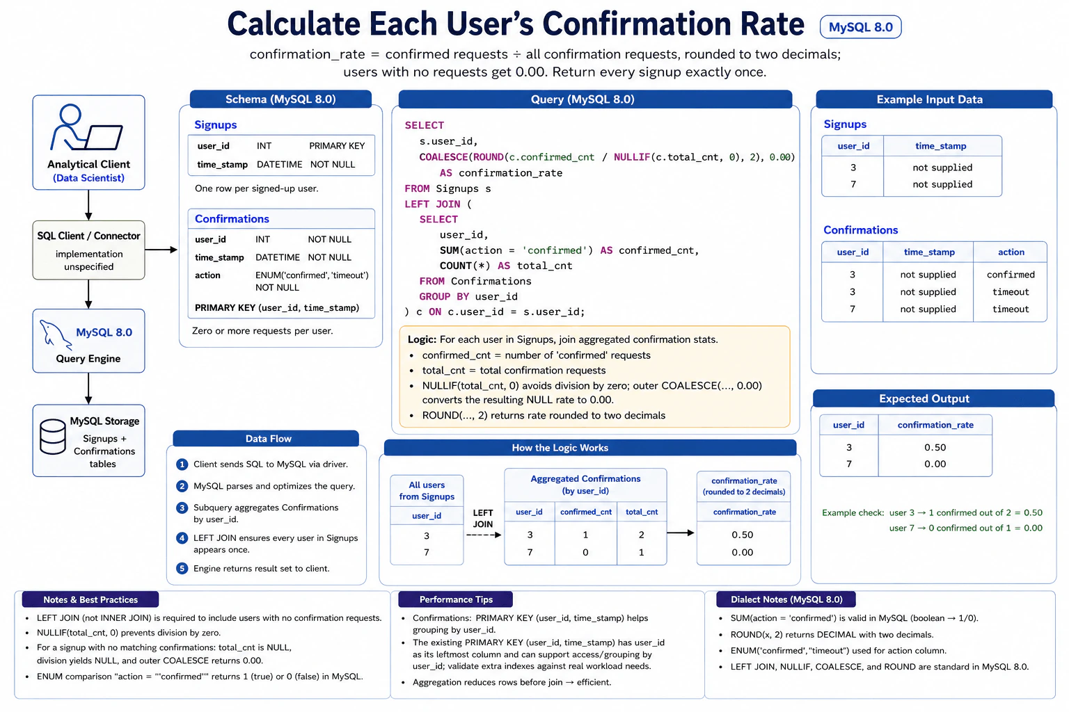
Use MySQL 8.0. Table Signups(user_id INT PRIMARY KEY, time_stamp DATETIME NOT NULL) has one row per signed-up user. Table Confirmations(user_id INT NOT NULL, time_stamp DATETIME NOT NULL, action ENUM('confirmed','timeout') NOT NULL, PRIMARY KEY(user_id,time_stamp)) has zero or more requests per user. Return every signup once with user_id and confirmation_rate, defined as confirmed requests divided by all confirmation requests, rounded to two decimals; users with no requests get 0.00. Row order is unrestricted. Example signups 3 and 7 with confirmations (3,confirmed),(3,timeout),(7,timeout) must return rates 0.50 and 0.00.
Short Interview Answer (30-60 seconds)
Aggregate Confirmations by user_id, counting confirmed requests and all requests. LEFT JOIN those counts to Signups so every signup remains. Divide confirmed_cnt by total_cnt with NULLIF for safe division, wrap the rounded result with COALESCE, and return 0.00 when a user has no requests.
We need to give one result for every person who signed up. For each person, look at all confirmation requests and count how many succeeded. Divide the successful count by the total number of requests and show the result with two decimal places. A person who never made a confirmation request must still appear and must receive 0.00. In the example, user 3 succeeded once out of two requests, so the result is 0.50. User 7 had one request and it did not succeed, so the result is 0.00.
Useful Questions to Ask the Interviewer
Is there an expected data-size or performance boundary that should influence whether we discuss additional indexing or query-plan verification?
How to Explain It in an Interview
The required result grain is one row per signup. Signups.user_id is a primary key, so Signups already contains exactly one row per signed-up user. Confirmations has zero or more requests per user and has primary key (user_id, time_stamp).
First, aggregate Confirmations by user_id. In MySQL 8.0, SUM(action = 'confirmed') counts confirmed rows because the comparison evaluates to 1 when true and 0 when false. COUNT(*) counts all confirmation requests. This produces at most one aggregate row per user.
Next, LEFT JOIN that aggregate to Signups. The LEFT JOIN is essential because an INNER JOIN would remove signups that have no confirmation requests. If a signup has no matching aggregate row, confirmed_cnt and total_cnt are NULL.
Calculate c.confirmed_cnt / NULLIF(c.total_cnt, 0). NULLIF prevents division by zero. Then use ROUND(..., 2) and wrap the final expression with COALESCE(..., 0.00). For a signup with no matching confirmations, the division result is NULL and the outer COALESCE returns 0.00.
For the supplied example, user 3 has one confirmed request out of two total requests, so the rate is 0.50. User 7 has zero confirmed requests out of one total request, so the rate is 0.00. Row order is unrestricted, so no ORDER BY is required.
The existing Confirmations primary key (user_id, time_stamp) has user_id as its leftmost column, so it can support access and grouping by user_id. I would not add another index automatically. I would consider table size, data distribution, workload, and the MySQL execution plan before adding an index because extra indexes consume storage and increase write-maintenance cost.
Technical Approach
Use Signups as the base because every signup must appear exactly once.
Group Confirmations by user_id.
Compute confirmed_cnt with SUM(action = 'confirmed').
Compute total_cnt with COUNT(*).
LEFT JOIN the aggregated counts to Signups by user_id.
Divide confirmed_cnt by NULLIF(total_cnt, 0).
Round the ratio to two decimals.
Use outer COALESCE to return 0.00 when no confirmation aggregate exists.
Do not add ORDER BY because row order is unrestricted.
Practical Complexity & Trade-offs
Logically, the query processes the signup rows and the confirmation rows needed for aggregation. With S signups and C confirmation rows, the amount of work is roughly proportional to S + C, although MySQL may choose a different physical execution plan. Grouping requires working memory or temporary storage for per-user counts. The existing primary key (user_id, time_stamp) starts with user_id and can support access or grouping by user_id. Additional indexes consume storage and add write cost, so they should be justified by the real workload and execution plan.
Example
The subquery reduces Confirmations to one row per user before the join. SUM(action = 'confirmed') counts confirmed requests in MySQL 8.0, while COUNT(*) counts all requests. LEFT JOIN preserves every signup. NULLIF(total_cnt, 0) protects the denominator, ROUND(..., 2) rounds the rate, and the outer COALESCE converts a missing rate to 0.00. Because the aggregate has at most one row per user and Signups has a primary key on user_id, the final result has exactly one row per signup.
Code
-- Start from Signups so the final result grain is exactly one row per signed-up user.SELECT
s.user_id,
-- Protect the denominator with NULLIF, round to two decimals,-- and return 0.00 when the LEFT JOIN finds no confirmation aggregate.COALESCE(
ROUND(c.confirmed_cnt /NULLIF(c.total_cnt, 0), 2),
0.00
) AS confirmation_rate
FROM
Signups AS s
LEFTJOIN (
-- Aggregate Confirmations first so this subquery returns at most one row per user_id.SELECT
user_id,
-- In MySQL 8.0, the comparison is 1 for 'confirmed' and 0 otherwise.SUM(action ='confirmed') AS confirmed_cnt,
-- Count every confirmation request for the user.COUNT(*) AS total_cnt
FROM
Confirmations
GROUPBY
user_id
) AS c
-- LEFT JOIN keeps signups that have zero confirmation requests.ON c.user_id = s.user_id;
Where it is used
This pattern is common in product and behavioral analytics where every entity must remain in the result even when it has no activity. Examples include signup-to-verification rates, email-confirmation rates, payment-success rates, application-completion rates, experiment conversion summaries, and other success-count divided by attempt-count metrics.
Why Interviewers Ask This
This question tests whether the candidate can preserve the required one-row-per-signup result grain while calculating a ratio from a one-to-many relationship. It checks aggregation, LEFT JOIN behavior, MySQL conditional counting, NULL handling, safe division, rounding, keys, and practical indexing judgment.
Common interview mistakes
Using INNER JOIN is a major mistake because it removes signups with no confirmation requests. Another mistake is counting all rows after a direct LEFT JOIN with COUNT(*), which can incorrectly count the preserved signup row even when no confirmation exists. Candidates may also divide without safe NULL or zero handling, forget the required 0.00 default, forget to round to two decimals, accidentally change the one-row-per-signup grain, add unnecessary ordering, or recommend another index without considering that the existing (user_id, time_stamp) primary key already begins with user_id.
Interview tip
State the required grain first: one row per signup. Then explain why you aggregate Confirmations before the LEFT JOIN. Walk through the no-request case explicitly: the joined counts are NULL, NULLIF keeps division safe, and outer COALESCE returns 0.00. Finish by checking users 3 and 7 against 0.50 and 0.00.
Interviewer may ask next
Why use a LEFT JOIN instead of an INNER JOIN?
The requirement says every signup must appear, including users with zero confirmation requests. An INNER JOIN would keep only users with a matching confirmation aggregate, so users with no requests would disappear. A LEFT JOIN keeps every row from Signups; missing confirmation counts become NULL, and the final COALESCE converts the missing rate to 0.00.
Would you add an index on Confirmations(user_id) for this query?
Not automatically. The existing primary key is (user_id, time_stamp), so user_id is already the leftmost indexed column and can support access or grouping by user_id. Whether another index helps depends on table size, data distribution, workload, and the plan MySQL chooses. I would inspect the execution plan and workload evidence before adding an index because every extra index uses storage and adds write-maintenance cost.
73. Return employees whose salaries are among the top three distinct salaries in their department.Sql And DatabaseHard
i Question Details
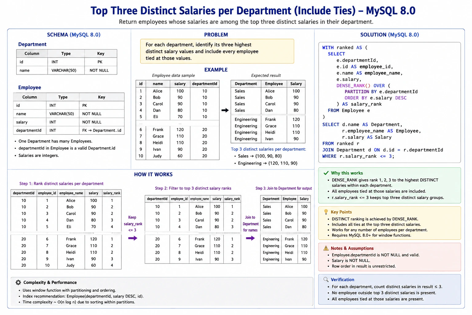
Use MySQL 8.0. Table Department(id INT PRIMARY KEY, name VARCHAR(50) NOT NULL) has one row per department. Table Employee(id INT PRIMARY KEY, name VARCHAR(50) NOT NULL, salary INT NOT NULL, departmentId INT NOT NULL) has valid department keys. For each department, identify its three highest distinct salary values and include every employee tied at those values. Return columns named Department, Employee, and Salary; row order is unrestricted and duplicate employees do not occur. If a department has salaries 100, 90, 90, 80, and 70, include the employees at 100, both at 90, and the employee at 80.
Short Interview Answer (30-60 seconds)
Use DENSE_RANK() partitioned by departmentId and ordered by salary descending. Tied salaries receive the same rank, so filtering to ranks 1 through 3 keeps the three highest distinct salary levels and every employee tied at those levels. Then join Department to return its name.
The task is to examine each department separately and find its three highest different salary amounts. Every employee earning one of those amounts must be returned. Employees with the same salary belong to the same salary level, so a department can return more than three people. For salaries 100, 90, 90, 80, and 70, the selected levels are 100, 90, and 80. Both employees earning 90 remain in the result. The final output contains the department name, employee name, and salary, with no required row order.
Useful Questions to Ask the Interviewer
Should every employee tied at the third-highest distinct salary be included? Yes, the requirement explicitly says to include all ties.
What should happen when a department has fewer than three distinct salary values? Return employees at every salary level that exists.
Is a particular final row order required? No. The question says row order is unrestricted.
How to Explain It in an Interview
Use MySQL 8.0's DENSE_RANK() window function. A window function calculates a value across related rows while keeping the original rows instead of collapsing them into groups.
Partition by departmentId, so ranking restarts for every department. Inside each partition, order by salary DESC so the highest salary receives rank 1. DENSE_RANK() assigns the same rank to equal salaries and does not leave gaps between distinct salary levels.
For example, salaries 100, 90, 90, 80, and 70 receive ranks 1, 2, 2, 3, and 4. Filtering to salary_rank <= 3 therefore returns the employee at 100, both employees at 90, and the employee at 80. This exactly matches the requirement to keep the top three distinct salary values while including every tie.
The ranked result stays at employee grain: one row per employee. Join Department using Department.id = Employee.departmentId to obtain the department name. Because every employee has a valid department key, this many-to-one join does not duplicate employee rows. Return d.name AS Department, the employee name as Employee, and salary as Salary.
The schema defines salary and departmentId as NOT NULL, so no special null handling is needed. Employee IDs are primary keys and duplicate employees do not occur, so no final DISTINCT is needed. Row order is unrestricted, so an outer ORDER BY is unnecessary.
For performance, the main cost is partitioning and ordering employees for the window function. An index such as Employee(departmentId, salary DESC, id) can support relevant access and ordering patterns, but indexes consume storage and add write-maintenance cost. MySQL's optimizer chooses the physical execution plan, so use EXPLAIN with representative data when production performance matters.
Technical Approach
1. Start with Employee at one row per employee. 2. Partition rows by departmentId. 3. Order salaries descending within each department. 4. Apply DENSE_RANK() so equal salaries receive the same rank and distinct salary levels receive consecutive ranks. 5. Keep rows with salary_rank <= 3. 6. Join Department on Department.id = departmentId. 7. Return Department, Employee, and Salary. 8. Do not add DISTINCT or a final ORDER BY because duplicate employees do not occur and output order is unrestricted.
Practical Complexity & Trade-offs
The main work is ranking employee salaries inside each department. In the general case, ordering N employee rows can require about O(N log N) work, although the actual MySQL execution plan depends on data distribution and available indexes. The window operation may also use working memory or temporary storage. The Department join is efficient because Department.id is a primary key. An index such as Employee(departmentId, salary DESC, id) may help the access and ordering pattern, but it consumes storage and adds maintenance work when Employee rows are inserted or updated. Use EXPLAIN to verify the real plan rather than assuming an index removes every sort.
Example
The common table expression keeps one row per employee and calculates a salary rank within that employee's department. PARTITION BY e.departmentId restarts the ranking for each department, while ORDER BY e.salary DESC ranks higher salaries first. DENSE_RANK() gives employees with equal salaries the same rank and gives the next distinct salary the next consecutive rank. The outer query joins Department to obtain its name and filters to ranks 1, 2, and 3. The schema already excludes null salaries and invalid department keys, duplicate employees do not occur, and the requested output has no required ordering.
Code
WITH
ranked AS (
SELECT
e.departmentId,
e.name AS employee_name,
e.salary,
-- Rank salary levels independently inside each department.-- DENSE_RANK gives tied salaries the same rank and keeps ranks consecutive.DENSE_RANK() OVER (
PARTITIONBY
e.departmentId
ORDERBY
e.salary DESC
) AS salary_rank
FROM
Employee AS e
-- Result grain remains one row per employee because Employee.id is a primary key.-- salary and departmentId are NOT NULL, so no special null handling is required.
)
SELECT
d.name AS Department,
r.employee_name AS Employee,
r.salary AS Salary
FROM
ranked AS r
JOIN Department AS d
-- Each employee has one valid department key, so this is a many-to-one join.ON d.id = r.departmentId
-- Keep the three highest distinct salary groups and every employee tied within them.WHERE
r.salary_rank <=3;
-- No final ORDER BY is required because result order is unrestricted.
Where it is used
This pattern is used for top-N-with-ties analysis within groups, such as finding employees in the highest compensation bands per department, top product prices per category, highest customer scores per segment, or strongest metric values per region. It is especially useful when the limit applies to distinct ranked values and all records tied at those values must remain.
Why Interviewers Ask This
This question tests whether the candidate understands ranking within groups, distinct value ranking, tie handling, window functions, many-to-one joins, result grain, and practical query performance. The key judgment is recognizing that the requirement is for the top three distinct salary values rather than exactly three employee rows, making DENSE_RANK() the appropriate ranking function.
Common interview mistakes
Using ROW_NUMBER() is incorrect because employees with equal salaries receive different row numbers, so tied employees can be dropped. Using RANK() with <= 3 is also incorrect for this exact requirement because gaps after ties can prevent the third distinct salary from qualifying; for 100, 90, 90, 80, 70 it produces ranks 1, 2, 2, 4, 5. Using LIMIT 3 returns at most three rows rather than three distinct salary levels. Forgetting PARTITION BY departmentId ranks salaries across the whole company instead of within each department. Forgetting the Department join fails to return the required department name. Adding DISTINCT is unnecessary because duplicate employees do not occur.
Interview tip
Start by saying that the requirement is for three distinct salary levels, not three employee rows. Then explain why DENSE_RANK() matches that rule: tied salaries share one rank and the next distinct salary gets the next consecutive rank. Walk through 100, 90, 90, 80, 70 as ranks 1, 2, 2, 3, 4.
Interviewer may ask next
Why is DENSE_RANK() better than ROW_NUMBER() or RANK() for this requirement?
DENSE_RANK() directly represents distinct salary levels. Equal salaries receive the same rank, and the next different salary receives the next consecutive rank. For 100, 90, 90, 80, and 70, it produces 1, 2, 2, 3, 4. ROW_NUMBER() would number tied employees separately and could remove a tie when filtered to three. RANK() would produce 1, 2, 2, 4, 5, so rank <= 3 would incorrectly omit 80 even though 80 is the third-highest distinct salary.
What happens when a department has fewer than three distinct salaries, and what index would you consider?
Every employee in that department is returned because all existing distinct salary levels have DENSE_RANK values of 1, 2, or 3. For performance, an index such as Employee(departmentId, salary DESC, id) may support the partition-and-order access pattern. It also consumes storage and adds write-maintenance cost, and MySQL may still choose a plan that performs sorting. Validate the actual behavior with EXPLAIN and representative data.
74. Calculate daily cancellation rates for trips requested by unbanned users.Sql And DatabaseHard
i Question Details
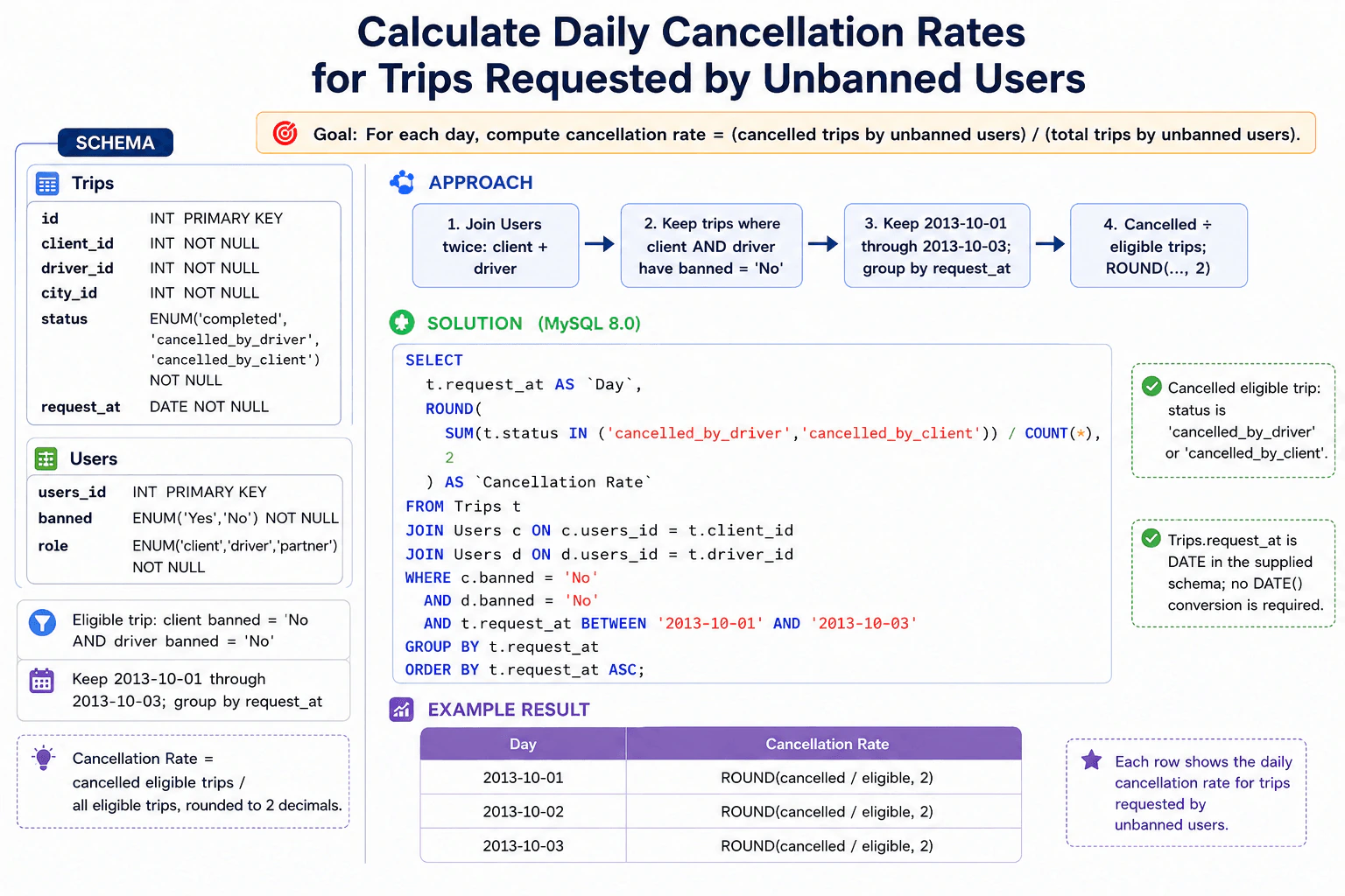
Use MySQL 8.0. Table Trips(id INT PRIMARY KEY, client_id INT NOT NULL, driver_id INT NOT NULL, city_id INT NOT NULL, status ENUM('completed','cancelled_by_driver','cancelled_by_client') NOT NULL, request_at DATE NOT NULL) has one row per trip. Table Users(users_id INT PRIMARY KEY, banned ENUM('Yes','No') NOT NULL, role ENUM('client','driver','partner') NOT NULL) identifies users. For dates 2013-10-01 through 2013-10-03 inclusive, keep only trips whose client and driver are both unbanned. For each date with at least one eligible trip, return Day and Cancellation Rate, where the rate is cancelled eligible trips divided by all eligible trips, rounded to two decimals; sort by Day ascending.
Short Interview Answer (30-60 seconds)
Join Users twice to validate both the client and driver. Filter both to banned = 'No' and keep the required dates. Group by request_at, divide cancelled eligible trips by all eligible trips, round to two decimals, and order by Day ascending.
We need to look at trips made during three specific days and ignore any trip where either person involved is banned. For every remaining day, we count how many trips happened and how many ended because either the client or driver cancelled. We then divide the cancelled count by the total count for that day and round the result to two decimal places. A day appears only when at least one valid trip exists. Finally, the days must be returned from earliest to latest.
Useful Questions to Ask the Interviewer
Should both the client and driver be required to have banned = 'No'? Yes. The question explicitly requires both to be unbanned.
Should a date with no eligible trips appear with a zero cancellation rate? No. Only dates with at least one eligible trip should appear.
Is request_at already stored as a DATE? Yes. No date-extraction function is needed.
How to Explain It in an Interview
The required result grain is one row per request_at date that has at least one eligible trip. Trips contains one row per trip. Users.users_id is a primary key, so each client or driver identifier can match at most one Users row.
I join Users twice because client_id and driver_id represent two different people. The client alias joins on c.users_id = t.client_id, and the driver alias joins on d.users_id = t.driver_id. I then keep only trips where both c.banned = 'No' and d.banned = 'No'.
The date filter is inclusive: t.request_at BETWEEN '2013-10-01' AND '2013-10-03'. Because request_at is already a DATE, there is no need to wrap it in DATE().
A trip counts as cancelled when status is either cancelled_by_driver or cancelled_by_client. In MySQL, the expression t.status IN (...) evaluates to 1 when true and 0 when false, so summing it counts cancelled eligible trips. COUNT(*) counts every eligible trip in the same daily group. Dividing the cancelled count by COUNT(*) gives the requested cancellation rate, and ROUND(..., 2) rounds it to two decimal places.
There is no divide-by-zero case for an emitted group because a GROUP BY row exists only when at least one eligible trip survived the joins and filters. Finally, ORDER BY t.request_at ASC returns the result from earliest to latest.
The supplied schema represents only the current banned value. It contains no ban-history timestamp, so I would not invent historical ban-state logic.
Technical Approach
Start from Trips, which has one row per trip.
Join Users as the client with c.users_id = t.client_id.
Join Users again as the driver with d.users_id = t.driver_id.
Keep only rows where c.banned = 'No' and d.banned = 'No'.
Keep trips from 2013-10-01 through 2013-10-03 inclusive.
Group the eligible trips by t.request_at.
Count cancelled trips by summing the condition that status is cancelled_by_driver or cancelled_by_client.
Divide cancelled eligible trips by all eligible trips and round to two decimals.
Return exactly Day and Cancellation Rate, ordered by day ascending.
Practical Complexity & Trade-offs
The database must find trips in the requested date range, look up the client and driver for each relevant trip, and aggregate the eligible rows by day. The two Users joins are primary-key lookups because users_id is the primary key. An index that starts with request_at may help a large Trips table avoid reading unrelated dates, but the actual benefit should be checked with the query plan. Only a few daily groups are produced here, so aggregation memory is small. No application-side transaction logic is needed for this single read query, and maintenance cost is low because the query follows the supplied schema directly.
Example
The query joins Users twice because every trip has both a client and a driver whose ban status must be checked independently. The WHERE clause applies both eligibility filters and the inclusive three-day date range before aggregation. Because request_at is already a DATE, it is grouped directly. The conditional SUM counts the two cancellation statuses, while COUNT(*) counts every eligible trip in the daily group. Their quotient is rounded to two decimals. The final ORDER BY returns the required ascending day order.
Code
-- Result grain: one row per request date that has at least one eligible trip.SELECT
t.request_at ASDAY,
-- Count cancelled eligible trips, divide by all eligible trips for the day,-- and round the requested ratio to two decimal places.
ROUND(
SUM(
t.status IN ('cancelled_by_driver', 'cancelled_by_client')
) /COUNT(*),
2
) AS Cancellation Rate
FROM
Trips AS t
-- Join the client through the Users primary key.JOIN Users AS c ON c.users_id = t.client_id
-- Join Users independently for the driver because driver eligibility is also required.JOIN Users AS d ON d.users_id = t.driver_id
-- Both participants must be unbanned, and the requested date range is inclusive.WHERE
c.banned ='No'AND d.banned ='No'AND t.request_at BETWEEN'2013-10-01'AND'2013-10-03'-- request_at is already DATE, so group directly at the required daily grain.GROUPBY
t.request_at
-- Return days from earliest to latest.ORDERBY
t.request_at ASC;
Where it is used
This pattern is common in transportation, delivery, marketplace, booking, and platform analytics. It is useful whenever an event references multiple participants and a metric should include the event only when every required participant satisfies an eligibility rule. The same conditional-aggregation idea can also calculate daily failure rates, refund rates, defect rates, or other ratios.
Why Interviewers Ask This
This question tests whether you can translate several business rules into precise SQL. The key judgment is recognizing that eligibility depends on both the client and the driver, so Users must be joined twice. It also tests correct filtering, daily aggregation, conditional counting, numerical division, rounding, result grain, and ordering without inventing columns or changing the supplied schema.
Common interview mistakes
Common mistakes are checking only the client and forgetting that the driver must also be unbanned; joining Users only once; using banned = 0 even though the supplied column is ENUM('Yes','No'); inventing a banned_at column; forgetting one of the two cancellation statuses; multiplying the ratio by 100 even though the question asks for a rate rather than a percentage; wrapping request_at in an unnecessary DATE() call; omitting the inclusive date filter; returning extra columns instead of exactly Day and Cancellation Rate; or forgetting the ascending sort.
Interview tip
State the output grain first: one row per eligible day. Then explain the key insight that Users must be joined twice because both the client and driver must be unbanned. Finish by defining the cancellation numerator, the eligible-trip denominator, the two-decimal rounding, and the ascending order.
Interviewer may ask next
How would the query change if every date had to appear even when there were no eligible trips?
Use a date source containing the required dates and LEFT JOIN the daily eligible-trip aggregation to it. For a date with no eligible trips, the denominator is zero, so the interviewer must define whether the cancellation rate should be NULL, 0, or another value. The original question avoids this ambiguity by returning only dates with at least one eligible trip.
What indexes could help if Trips were very large?
The Users joins already use the users_id primary key. On Trips, an index beginning with request_at may help restrict work to the requested dates. Whether a wider composite index is worthwhile depends on data distribution and the optimizer's plan, so I would inspect EXPLAIN before claiming a specific index is best.
75. What is Big O notation, and why does it matter when processing large datasets?CodingEasy
i Question Details
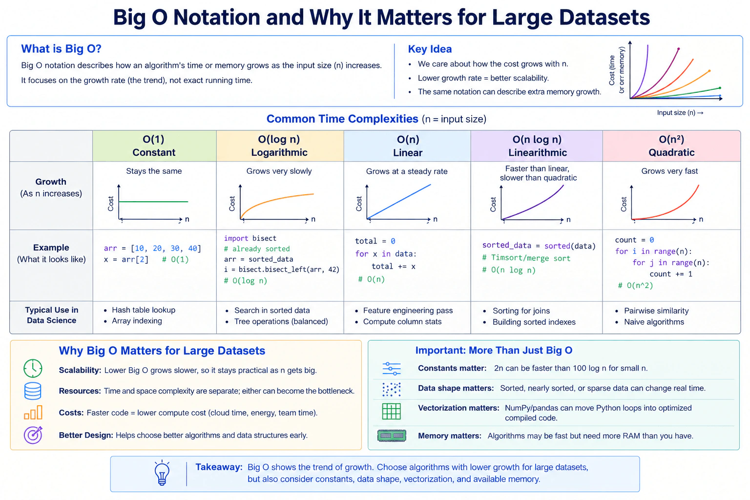
Explain how Big O notation describes the growth of runtime and memory requirements as input size increases. Compare constant, logarithmic, linear, linearithmic, and quadratic complexity using short Python or data-processing examples, and explain why constants, data shape, vectorization, and available memory still matter in practice.
Short Interview Answer (30-60 seconds)
Big O notation describes how runtime or memory grows as the input size n becomes larger. I compare growth rates such as O(1), O(log n), O(n), O(n log n), and O(n²). For example, array indexing is O(1), binary search on sorted data is O(log n), scanning rows is O(n), sorting is O(n log n), and comparing every pair is O(n²). Lower growth usually scales better, but constants, data shape, vectorization, and available memory still matter in practice.
The question asks how the amount of work or memory changes when a dataset becomes larger. Big O gives us a simple way to describe that growth. It does not predict an exact number of seconds or bytes. Instead, it shows the trend as the input size n increases. The diagram compares constant, logarithmic, linear, linearithmic, and quadratic growth. It also shows why theoretical growth is only part of the decision because real performance depends on constants, data shape, vectorized execution, and available memory.
Useful Questions to Ask the Interviewer
Should I discuss both runtime complexity and space complexity?
Should I compare the five common growth rates with Python examples?
Should I also explain practical factors such as vectorization and available RAM?
How to Explain It in an Interview
1. Start with the meaning of Big O
Big O describes how a cost grows when input size n grows. The cost can be execution time or memory usage. It focuses on the growth trend rather than exact runtime.
Time complexity and space complexity are separate. The same Big O notation can describe either one. An algorithm may have acceptable runtime growth but still need more memory than the machine has.
2. Compare the five complexity classes
O(1) is constant complexity. Its cost stays roughly the same as n grows. The diagram shows direct array access with arr = [10, 20, 30, 40] and x = arr[2].
O(log n) is logarithmic complexity. It grows very slowly. The diagram uses binary search on data that is already sorted. With bisect.bisect_left, the search repeatedly narrows the remaining range instead of scanning every item.
O(n) is linear complexity. The work grows in direct proportion to the number of input items. The diagram shows a loop that scans all rows and adds each value to total.
O(n log n) is linearithmic complexity. It grows faster than O(n) but much more slowly than O(n²). The diagram shows sorted_data = sorted(data), representing efficient comparison sorting such as Timsort or merge sort behavior.
O(n²) is quadratic complexity. The diagram shows two nested loops. Each of the n outer iterations performs n inner iterations, so the total number of iterations grows as n².
3. Connect each class to data-science work
O(1) examples include array indexing and average-case hash-table lookup. O(log n) appears in binary search on sorted data and balanced-tree operations. O(n) appears when scanning rows, computing column statistics, or performing one feature-engineering pass. O(n log n) appears when sorting for joins or building sorted indexes. O(n²) appears in pairwise similarity calculations and naive algorithms that compare every item with every other item.
4. Explain why growth matters for large datasets
For a small dataset, several approaches may all finish quickly. The difference becomes important when n grows to millions or billions of rows. Lower asymptotic growth usually scales better. It can reduce execution time, compute cost, and the risk that an approach becomes impractical as the dataset grows.
5. Explain why Big O is not the whole story
Constants matter. For a small n, an operation with a worse Big O class can still be faster because its constant overhead is lower.
Data shape matters too. Sorted, nearly sorted, sparse, duplicated, or skewed data can change real execution time.
Vectorization also matters. NumPy and pandas can move Python-level loops into optimized compiled code. This can reduce constant overhead even when the Big O class does not change.
Memory is another practical limit. Time and space complexity are separate. Either can become the bottleneck. An algorithm can be fast enough in theory but still fail because its data or temporary results do not fit in RAM.
6. Finish with the main takeaway
Big O helps compare how algorithms grow as data becomes larger. O(1), O(log n), and O(n) usually scale better than O(n²). But I would not choose an implementation from Big O alone. I would also consider constants, the shape of the data, vectorized execution, and available memory.
Key Insight / Why This Solution Works
This is a complexity-comparison question rather than one problem with one selected algorithm. The key idea is to hold the meaning of n constant as the input size and compare how different operations grow. The diagram uses direct array access for O(1), binary search on already sorted data for O(log n), a full scan for O(n), sorting for O(n log n), and nested all-pairs loops for O(n²). The central invariant is that each complexity label describes the growth trend of the shown operation as n increases. Lower growth usually scales better for very large inputs, but practical performance also depends on constant factors, data shape, vectorization, and memory limits.
Code
import bisect
# Shared small data used to make the diagram examples executable.
data = [10, 20, 30, 40]
# O(1): access one fixed array position.
arr = [10, 20, 30, 40]
x = arr[2]
# O(log n): binary search requires data that is already sorted.
sorted_data = [10, 20, 30, 40]
arr = sorted_data
# bisect_left repeatedly narrows the search range and returns an insertion position.
i = bisect.bisect_left(arr, 42)
# O(n): scan every item once and update the running total.
total = 0for x in data:
total += x
# O(n log n): create a sorted copy of the data.
sorted_data = sorted(data)
# O(n^2): perform one count update for every ordered pair of positions.
n = len(data)
count = 0for i inrange(n):
for j inrange(n):
count += 1
Time & Space Complexity
There is no single complexity for the whole answer because the diagram compares five different operations. Direct array access is O(1) time because one indexed lookup does not grow with n. Binary search on already sorted data is O(log n) time because each step removes a large part of the remaining search range. Scanning all items is O(n) time because every item is visited once. Sorting is O(n log n) time in the diagram. Two nested loops over n items are O(n²) time because they perform n × n iterations. The small examples shown use O(1) extra working memory apart from the sorted result, while Python sorted creates a new list whose size grows with n. Time and space complexity must be analyzed separately.
Where it is used
These ideas are used whenever a data scientist chooses between ways to process large data. Constant-time access appears in array indexing and average hash-table lookup. Logarithmic search appears with sorted data. Linear work appears in row scans, feature-engineering passes, and column statistics. Linearithmic work appears in sorting for joins and building sorted indexes. Quadratic work appears in pairwise similarity and naive all-pairs comparisons.
Why Interviewers Ask This
The interviewer is checking whether you can reason about scalability instead of judging code only on small inputs. They want to see whether you understand constant, logarithmic, linear, linearithmic, and quadratic growth and can connect each one to realistic data-processing work. They are also checking whether you separate runtime from memory complexity and understand that practical performance depends on more than asymptotic notation, especially constants, data shape, vectorization, and available memory.
Common interview mistakes
A common mistake is treating Big O as an exact runtime instead of a growth trend. Another mistake is counting the sorting step as part of the O(log n) binary-search example even though the diagram says the data is already sorted. Candidates may also assume one Big O value describes both time and memory, but time complexity and space complexity are separate. Another mistake is hiding the O(n log n) cost of sorting. Finally, lower Big O does not guarantee faster execution for every input because constants, data shape, vectorization, and hardware still affect real performance.
Interview tip
Explain the classes in increasing growth order and attach one concrete example to each one: array access, binary search, row scan, sorting, and all-pairs comparison. Then say that Big O describes growth, not exact runtime, and finish with the practical factors shown in the diagram.
Interviewer may ask next
Why can a vectorized O(n) NumPy operation be much faster than an O(n) Python loop?
Both can still be O(n) because the amount of work grows roughly in proportion to n. The difference is the constant overhead. A Python loop performs Python-level work for each item, while NumPy can move much of that work into optimized compiled code. The asymptotic class can stay O(n) even though the real runtime becomes much smaller. The tradeoff is that vectorized operations can sometimes create temporary arrays and use additional memory.
What should you consider if the runtime complexity is acceptable but the dataset does not fit in RAM?
I would analyze space complexity separately from time complexity. A method can have good runtime growth and still use too much memory. Depending on the task, I could process the data in chunks, stream records, avoid unnecessary copies, or use a method with lower working-memory requirements. The exact new time and space complexity depends on the chosen approach, so I would state both instead of assuming that reducing memory is free.
76. Return the indices of two numbers that add to a target.CodingEasy
i Question Details
Using Python 3.14, implement def two_sum(nums: list[int], target: int) -> list[int]. nums has length 2 to 10,000; each value and target is between -10^9 and 10^9. Exactly one pair of distinct indices has values summing to target; the same element may not be used twice. Return the two zero-based indices in either order as a new two-item list without mutating nums. Use only the Python standard library and target O(n) time. Inputs outside this contract need not be handled. Example: two_sum([2, 7, 11, 15], 9) returns [0, 1] or [1, 0].
Short Interview Answer (30-60 seconds)
I use a hash map that stores each earlier value and its index. For each number, I calculate its complement, which is the target minus the current value. I check for that complement before storing the current number, so I cannot reuse the same element. When the complement exists, I return the two indices immediately. I process each item at most once and stop when the answer is found. This gives O(n) expected time and O(n) auxiliary space.
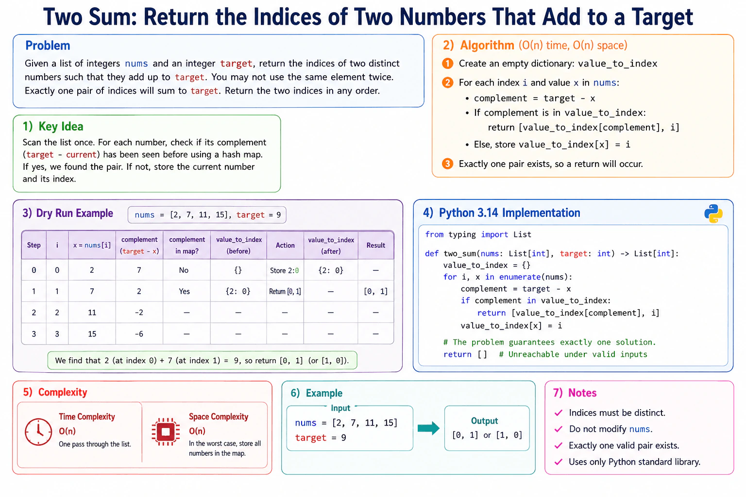
We are given a list of integers called nums and an integer target. We need the zero-based positions of two different elements whose values add up to target. The list has between 2 and 10,000 elements. Each value and target is between -10^9 and 10^9. Exactly one valid pair is guaranteed. Either index order is accepted. We must return a new two-item list and must not change nums. A dictionary is a good fit because it lets us remember earlier values and quickly find the value needed for the target.
Useful Questions to Ask the Interviewer
Can I return the two valid indices in either order?
Is exactly one valid pair always guaranteed, as stated?
Should I leave the input list unchanged?
How to Explain It in an Interview
1. Understand the input and required output
The function receives nums, a list of integers, and target, an integer. It must return a new list containing two distinct zero-based indices. The values at those indices must add to target. The same element cannot be used twice. The input list must stay unchanged. Exactly one valid pair is guaranteed, and either order of the two indices is valid.
2. Choose the algorithm and data structure
I use a dictionary named value_to_index. It acts as a hash map. Each key is a value already processed. Its mapped value is that earlier element's index. Before processing index i, the map contains only values from earlier indices. For the current value x, I calculate complement = target - x. Complement means the value needed with x to reach target. If that complement is already in the map, I have found the required pair.
3. Initialize the state
I start with value_to_index = {}. Nothing has been processed yet, so the empty map is correct. Then I move from left to right through nums. For each element, I get both its index i and its value x.
4. Walk through the example
The example is nums = [2, 7, 11, 15] and target = 9.
At index 0, x = 2. The map before the step is {}. I calculate complement = 9 - 2 = 7. The value 7 is not in the map. I therefore store 2 -> 0. The map becomes {2: 0}.
At index 1, x = 7. The map before the step is {2: 0}. I calculate complement = 9 - 7 = 2. The value 2 is already in the map at index 0. I return [0, 1] immediately. Processing stops, so indices 2 and 3 are not processed.
The returned indices point to nums[0] = 2 and nums[1] = 7. Their values satisfy 2 + 7 = 9. Therefore, [0, 1] is a correct returned pair. [1, 0] is also allowed because the problem accepts either order.
5. Explain why the result is correct
The important invariant is that value_to_index contains only values from earlier indices. I check for the complement before storing the current value. Therefore, when a complement is found, its stored index must be different from the current index. Also, complement + x equals target by definition. Because the problem guarantees one valid pair, the algorithm eventually finds that pair and returns it.
6. Explain the Python implementation
The code creates an empty dictionary. enumerate(nums) gives the current index and value. For each value, the code calculates target - x. It looks for that complement before inserting x. If the complement exists, it returns the earlier index and the current index immediately. Otherwise, it stores the current value and index for later elements. The final return [] is only a defensive fallback. It is not expected for an input that follows the stated contract.
7. Explain complexity and edge cases
Python dictionary lookup and insertion are O(1) on average. We process the input at most once, so the total expected time is O(n). The dictionary can grow with the number of processed elements, so auxiliary space is O(n). Duplicate values work correctly because the current value is checked against earlier values before it is inserted. Negative numbers and zero also work. The algorithm does not mutate nums.
Key Insight / Why This Solution Works
The key idea is to remember values from earlier indices. The dictionary stores value -> earlier index. For each current value x, calculate complement = target - x. If complement is already stored, return the earlier index and the current index. Otherwise, store x with its index and continue. The central invariant is that the map contains only values from earlier indices. Checking before insertion prevents the current element from matching itself. This avoids the slower approach of checking every possible pair.
Code
deftwo_sum(nums: list[int], target: int) -> list[int]:
# Store each value already processed and the index where it appeared.
value_to_index: dict[int, int] = {}
# Process elements from left to right until the valid pair is found.for i, x inenumerate(nums):
# Complement is the value needed with x to reach the target.
complement = target - x
# Check before insertion so the current element cannot match itself.if complement in value_to_index:
# Return the earlier matching index and the current index.return [value_to_index[complement], i]
# No pair yet, so remember this value and its index for later elements.
value_to_index[x] = i
# Defensive fallback; the stated problem guarantees a solution.return []
Time & Space Complexity
Let n be the number of elements in nums. We process the input at most once. For each processed element, Python dictionary lookup and insertion are O(1) on average. Therefore, the total expected time is O(n). The dictionary may store up to O(n) values before the answer is found, so the auxiliary space is O(n). Auxiliary space means the extra memory used by the algorithm.
Where it is used
This pattern is useful when software needs to match a current item with something seen earlier while keeping original positions. Hash maps are commonly used for fast matching, deduplication, lookup-heavy data processing, and one-pass scans where repeated searching would be too slow.
Why Interviewers Ask This
This problem tests whether you can recognize a hash-map lookup pattern instead of checking every possible pair. It also tests whether you preserve original indices, keep values separate from indices, handle duplicates correctly, and maintain a clear invariant. The interviewer can also evaluate whether you understand early return behavior and whether you describe Python dictionary complexity accurately as average or expected rather than guaranteed constant-time behavior.
Common interview mistakes
A common mistake is returning the two values instead of their indices. Another mistake is storing the current value before checking its complement, which can allow the same element to be reused. Sorting nums without preserving original indices can also produce the wrong output. Candidates may continue processing after finding the pair instead of returning immediately. Another mistake is claiming guaranteed O(n) time instead of O(n) expected time for a Python dictionary-based solution.
Interview tip
Explain the invariant before coding: the dictionary contains only values from earlier indices. Then say that you check the complement before storing the current value. This makes it easy to explain why the two returned indices are always distinct.
Interviewer may ask next
What changes if a valid pair is not guaranteed?
The same hash-map scan can still be used. If no complement is found after processing the input, the function needs an agreed no-result value, such as an empty list or another sentinel required by the interface. The lookup-before-insertion rule and correctness invariant stay the same. Expected time remains O(n), and auxiliary space remains O(n). The main tradeoff is that the caller must now handle the no-solution result.
What happens with duplicate values, for example nums = [3, 3] and target = 6?
The same algorithm already handles this case. At index 0, complement is 3, but the dictionary is empty, so it stores 3 -> 0. At index 1, complement is again 3. The dictionary contains 3 -> 0, so the function returns [0, 1]. The two indices are distinct because the lookup happens before the current value is inserted. Expected time remains O(n), and auxiliary space remains O(n).
77. Determine whether two strings are anagrams.CodingEasy
i Question Details
Using Python 3.14, implement def is_anagram(s: str, t: str) -> bool. Both strings contain only lowercase English letters and each has length 1 to 50,000. Return True exactly when the strings contain identical character counts, including repeated letters; order does not matter. Treat the strings as immutable, use only the standard library, and do not normalize case or Unicode. Inputs outside the contract need not be handled. Example: is_anagram("anagram", "nagaram") returns True.
Short Interview Answer (30-60 seconds)
I would first compare the string lengths. If they differ, I return False. Otherwise, I create two arrays of 26 counters, one for each lowercase English letter. I scan each string and increment the matching counter using ord(ch) - ord('a'). At the end, I compare the two arrays. They are anagrams exactly when every character count matches. This takes O(n) time and O(1) auxiliary space because the arrays always contain exactly 26 counters.
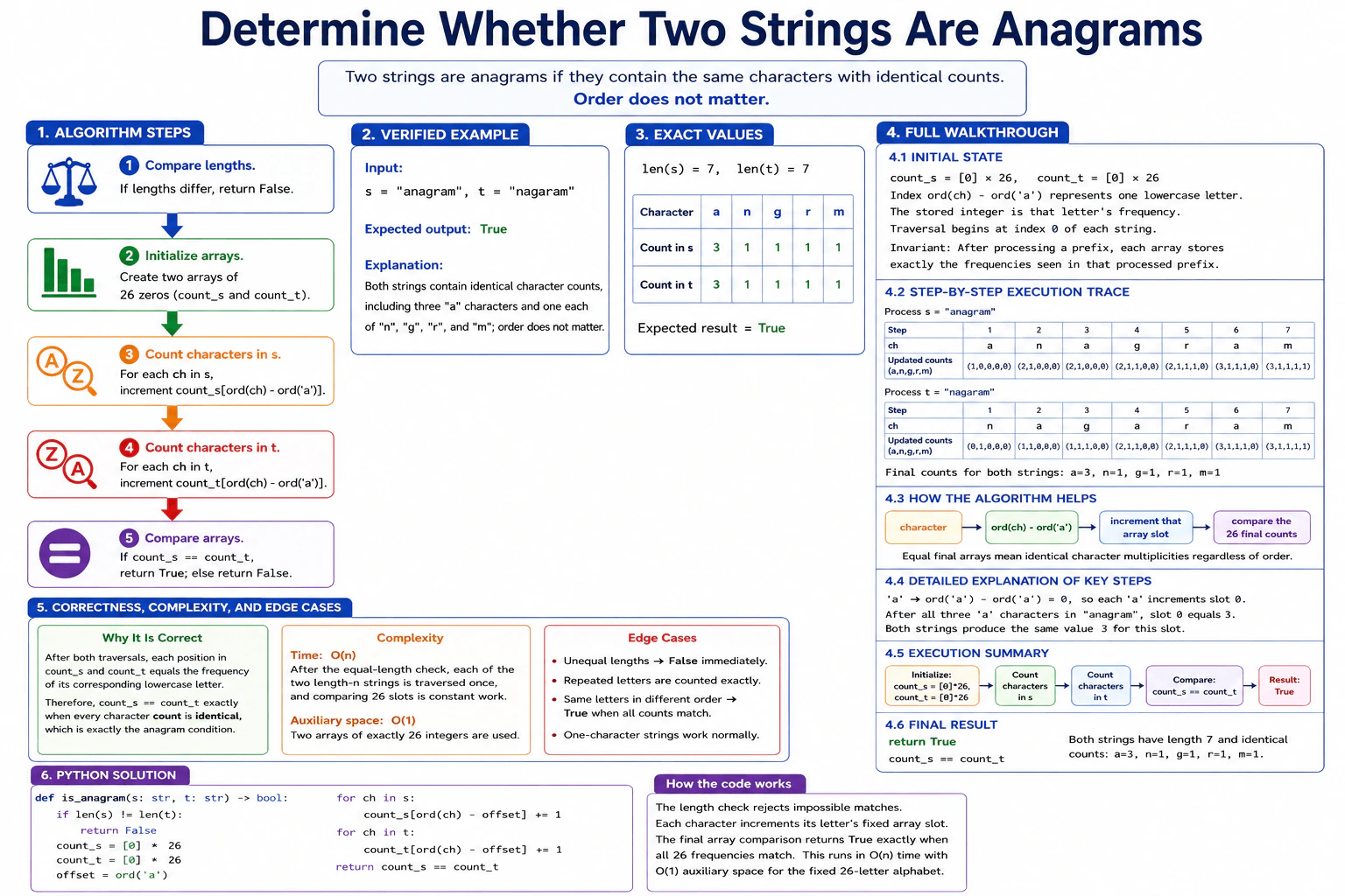
We need to decide whether two lowercase English strings contain exactly the same letters the same number of times. Their order does not matter. Repeated letters do matter. For example, "anagram" and "nagaram" are a match because both contain three "a" characters and one each of "n", "g", "r", and "m". I use two fixed arrays with 26 positions. Each position counts one lowercase letter. This fits the problem because the alphabet size is fixed.
Useful Questions to Ask the Interviewer
Can I assume both strings contain only lowercase English letters, as stated?
Should repeated letters count separately? Yes, identical frequencies are required.
Do I need to handle inputs outside the stated length and character constraints? No.
How to Explain It in an Interview
1. Understand the input and required output
The function receives two strings, s and t. Each contains only lowercase English letters and has length from 1 to 50,000. We return True only when every letter appears the same number of times in both strings. We treat both strings as immutable. We do not normalize case or Unicode because inputs outside the stated contract do not need to be handled.
2. Choose the algorithm and data structure
I use two arrays of exactly 26 integer counters. Each array position represents one lowercase English letter. Position 0 represents "a", position 1 represents "b", and so on. The expression ord(ch) - ord('a') converts a character into its array position. The key invariant is that after processing any prefix of a string, its count array stores exactly the letter frequencies seen in that processed prefix.
3. Initialize and process the strings
First, compare len(s) and len(t). If the lengths differ, return False immediately because strings with different numbers of characters cannot have identical character counts. Otherwise, create count_s = [0] * 26 and count_t = [0] * 26. Store ord('a') as offset. Then process every character in s and increment its position in count_s. Next, process every character in t and increment its position in count_t.
4. Walk through the verified example
For s = "anagram", the characters are processed in this order: a, n, a, g, r, a, m. The important final counts are a = 3, n = 1, g = 1, r = 1, and m = 1. For t = "nagaram", the characters are processed in this order: n, a, g, a, r, a, m. Its final counts are also a = 3, n = 1, g = 1, r = 1, and m = 1. For example, ord('a') - ord('a') = 0, so every "a" increments slot 0. After all three "a" characters are processed, slot 0 contains 3.
5. Explain why the result is correct
After both traversals, each position in count_s equals the frequency of its corresponding lowercase letter in s. The same is true for count_t and t. Therefore, count_s == count_t exactly when every character count is identical. That is exactly the definition required by this problem. For "anagram" and "nagaram", the arrays match, so the function returns True.
6. Explain complexity and edge cases
After the equal-length check, each length-n string is traversed once. Comparing the two 26-element arrays takes constant work because 26 does not grow with n. The total time is O(n). Auxiliary space is O(1) because the two arrays always contain exactly 26 integers. Unequal lengths return False immediately. Repeated letters are counted exactly. Different character order does not matter. One-character strings work normally.
Key Insight / Why This Solution Works
The key idea is to compare character frequencies instead of character positions. Because the contract limits every character to one of 26 lowercase English letters, two fixed arrays of 26 counters are enough. The expression ord(ch) - ord('a') maps each character to its counter position. The central invariant is: after processing a prefix of a string, its array contains exactly the frequencies of the letters in that processed prefix. After both strings are processed, they are anagrams exactly when the two arrays are equal.
Code
defis_anagram(s: str, t: str) -> bool:
# Different lengths cannot have identical character counts.iflen(s) != len(t):
returnFalse# Keep one fixed counter for each lowercase English letter in each string.
count_s = [0] * 26
count_t = [0] * 26# Use the code point for 'a' to map letters to indices 0 through 25.
offset = ord("a")
# Count every character in s without modifying the input string.for ch in s:
count_s[ord(ch) - offset] += 1# Count every character in t using the same mapping.for ch in t:
count_t[ord(ch) - offset] += 1# Equal arrays mean all 26 character frequencies are identical.return count_s == count_t
# Run the verified example from the problem and diagram.print(is_anagram("anagram", "nagaram")) # True
Time & Space Complexity
Let n be the length of each string after the initial length check confirms the lengths are equal. We read all n characters in s once and all n characters in t once. We then compare 26 counter positions. Since 26 is a fixed constant, this gives O(n) time. Auxiliary space is O(1) because count_s and count_t always contain exactly 26 integers, regardless of how large n becomes.
Where it is used
This fixed-frequency-array pattern is useful when software needs to compare counts from a small, known set of possible values. For example, it can compare lowercase text signatures or count fixed categories where the number of categories never grows with the input size.
Why Interviewers Ask This
This question checks whether you recognize that an anagram test is really a frequency-counting problem. It tests whether you choose a data structure that matches the fixed lowercase alphabet, handle repeated characters correctly, maintain a clear counting invariant, and write simple Python without unnecessary work. It also checks whether you can justify the early length check and explain why the fixed 26-element arrays give O(1) auxiliary space.
Common interview mistakes
A common mistake is checking only whether the same distinct letters appear while ignoring repeated counts. Another mistake is forgetting that different lengths can return False immediately. Candidates may also calculate the wrong array position for a character. Another error is changing the strings even though mutation is unnecessary. Finally, do not claim O(n) auxiliary space. The two counting arrays always have exactly 26 positions, so the auxiliary space is O(1).
Interview tip
Explain the invariant with one concrete mapping: 'a' gives ord('a') - ord('a') = 0, so every 'a' increments slot 0. Then explain that the same idea applies to all 26 lowercase letters. This makes the final count_s == count_t comparison easy to justify.
Interviewer may ask next
What would change if the strings could contain arbitrary Unicode characters instead of only lowercase English letters?
The fixed 26-element arrays would no longer represent every possible character. I would use frequency dictionaries instead. Each dictionary would map a character to its count. The correctness idea stays the same: the strings are anagrams exactly when every character frequency matches. With Python dictionaries, the expected time would be O(n), assuming average O(1) dictionary operations. Auxiliary space would become O(k), where k is the number of distinct characters. The tradeoff is support for a much larger character set at the cost of memory that can grow with the input.
Can we use one 26-element counting array instead of two?
Yes. Increment a letter's counter while scanning s and decrement the same counter while scanning t. At the end, every counter must be zero. A zero at every position means both strings contributed the same frequency for every lowercase letter, so correctness is preserved. The time remains O(n), and auxiliary space remains O(1). The main tradeoff is that one array uses slightly less constant memory, while the two-array version shown in the diagram can be easier to explain and inspect.
78. Validate a string of brackets.CodingEasy
i Question Details
Using Python 3.14, implement def is_valid(s: str) -> bool. s has length 1 to 10,000 and contains only (, ), [, ], {, and }. Return True exactly when every opening bracket is closed by the same type in properly nested order and no closing bracket appears without a matching opener. Do not mutate any caller-owned object; use only the standard library. Inputs outside the stated alphabet or length range need not be handled. Examples: is_valid("()[]{}") returns True, while is_valid("(]") returns False.
Short Interview Answer (30-60 seconds)
I would use a stack to keep the opening brackets that still need a match. I process each character at most once and stop immediately if the string becomes invalid. I push each opener. For a closer, the stack must be nonempty, and its top must be the matching opener. After all characters are processed, the stack must be empty. This works because nested brackets close in reverse order. The time complexity is O(n), and the auxiliary space is O(n).
The input is one string containing only round, square, and curly brackets. We need to return True only when every opening bracket has the correct closing bracket and the brackets are nested in the correct order. A closing bracket cannot appear without an opening bracket waiting for it. A stack fits this rule because the most recently opened bracket must be closed first. We read the string from left to right and never modify the input string.
Useful Questions to Ask the Interviewer
Can I rely on the stated guarantee that the input contains only (, ), [, ], {, and } and has length from 1 to 10,000?
Is O(n) auxiliary space acceptable for a stack when the input can contain many unmatched opening brackets?
How to Explain It in an Interview
1. Understand the input and required output
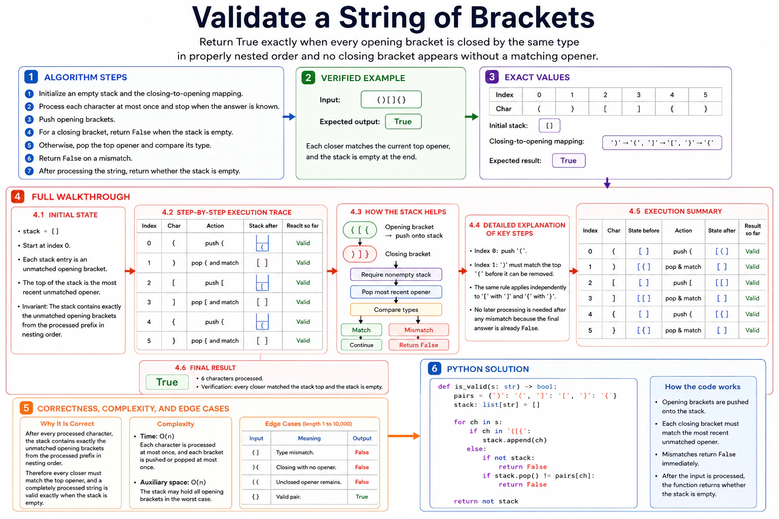
The function is is_valid(s: str) -> bool. The input is a string of length 1 to 10,000 containing only the six allowed bracket characters. We return True exactly when every opening bracket is closed by the same type in properly nested order and no closing bracket appears without a matching opener. The solution uses only the Python standard library and does not mutate any caller-owned object. The diagram's main example is "()[]{}", which returns True.
2. Choose the stack and matching rule
I use a stack. Each stack entry is an opening bracket that has not been matched yet. The top of the stack is the most recent unmatched opener. I also use the closing-to-opening mapping ')' -> '(', ']' -> '[', and '}' -> '{'.
The central invariant is: after every processed character, the stack contains exactly the unmatched opening brackets from the processed prefix, in nesting order. Because nested brackets must close in reverse order, each closer must match the stack top.
3. Initialize the state
Start with stack = []. Traversal begins at index 0. The stack is empty because no opening bracket has been processed yet. The dictionary pairs tells us which opening bracket is required for each closing bracket.
4. Walk through the example
For s = "()[]{}", the characters are at indices 0 through 5.
At index 0, the character is (. The stack is []. This is an opening bracket, so push it. The stack becomes ['(']. Processing continues.
At index 1, the character is ). The stack is ['(']. It is nonempty, so pop the top value (. The mapping says ) requires (. They match, so the stack becomes []. Processing continues.
At index 2, the character is [. Push it. The stack changes from [] to ['['].
At index 3, the character is ]. Pop [. The mapping says ] requires [. They match, so the stack becomes [].
At index 4, the character is {. Push it. The stack changes from [] to ['{'].
At index 5, the character is }. Pop {. The mapping says } requires {. They match, so the stack becomes [].
All 6 characters were processed. Every closing bracket matched the current stack top, and the stack is empty at the end. Therefore the function returns True. If a closer appeared while the stack was empty, or if a popped opener had the wrong type, the function would return False immediately and no later characters would be processed.
5. Explain why the result is correct
The stack always represents the opening brackets that still need a closing bracket. Its top is the most recent unmatched opener. Checking every closer against that top verifies both bracket type and nesting order. The empty-stack check prevents a closing bracket from appearing without an opener. Finally, an empty stack after the loop proves that no opening bracket was left unmatched.
6. Explain the Python implementation
The code first creates pairs, which maps every closing bracket to the opener it requires. It then creates an empty list called stack. Python lists support the needed stack operations with append and pop.
The loop processes the input from left to right. If ch is one of (, [, or {, the code pushes it. Otherwise, under the stated input guarantee, ch is a closing bracket. The code first checks if not stack so it never pops an empty stack. It then pops the most recent opener and compares it with pairs[ch]. Either failure returns False immediately. After the loop, return not stack returns True exactly when every opener was matched.
7. Explain complexity and edge cases
Let n be the length of the string. The time complexity is O(n). Each character is processed at most once, and each bracket is pushed or popped at most once. The auxiliary space complexity is O(n) because the stack can hold all opening brackets in the worst case.
Relevant edge cases from the diagram are "(]" -> False for a type mismatch, ")(" -> False for a closing bracket with no opener, "((" -> False because unmatched openers remain at the end, and "{}" -> True for a valid pair.
Key Insight / Why This Solution Works
Bracket nesting follows last-in, first-out order. The most recent unmatched opening bracket must be closed before any earlier opener, so a stack is the correct data structure. Opening brackets are pushed onto the stack. For each closing bracket, the stack must first be nonempty. Then the algorithm pops the most recent opener and checks it against the closing-to-opening mapping. The invariant is that the stack contains exactly the unmatched opening brackets from the processed prefix in nesting order. If the full input is processed and the stack is empty, every bracket was matched correctly.
Code
defis_valid(s: str) -> bool:
# Map each closing bracket to the opening bracket it must match.
pairs = {")": "(", "]": "[", "}": "{"}
# Store opening brackets that have not been matched yet.
stack: list[str] = []
# Process the input from left to right and stop on the first invalid state.for ch in s:
# An opening bracket waits for a matching closer later in the string.if ch in"([{":
stack.append(ch)
else:
# A closing bracket is invalid when there is no unmatched opener.ifnot stack:
returnFalse# The closer must match the most recent unmatched opening bracket.if stack.pop() != pairs[ch]:
returnFalse# Any opener left on the stack is unmatched, so only an empty stack is valid.returnnot stack
# Diagram example: this evaluates to True.
is_valid("()[]{}")
Time & Space Complexity
Let n be the length of the string. The time complexity is O(n). We process each character at most once. Each opening bracket can be pushed once, and each matched opening bracket can be popped once. The auxiliary space is O(n). Auxiliary space means extra memory used by the algorithm. In the worst case, the string can contain many opening brackets before any are closed, so the stack can grow to O(n) entries.
Where it is used
This stack pattern is useful when items must be closed or completed in reverse order from how they were opened. Common examples include validating brackets in source code, checking nested expressions, and parsing structures where the most recently opened construct must finish first.
Why Interviewers Ask This
This problem tests whether you recognize a last-in, first-out pattern and select a stack. It also checks whether you can maintain a clear invariant, validate both bracket type and nesting order, avoid popping an empty stack, and use early returns correctly. The interviewer can also evaluate whether you write simple Python, reason about edge cases such as unmatched openers and closers, and explain the O(n) time and O(n) auxiliary space accurately.
Common interview mistakes
A common mistake is checking only whether the counts of opening and closing brackets are equal. Equal counts do not prove correct type or nesting. Another mistake is popping before checking whether the stack is empty. Candidates may also compare a closing bracket with something other than the stack top, which breaks nesting order. Another error is forgetting the final empty-stack check, which would incorrectly accept inputs such as "((". Finally, once an empty-stack failure or type mismatch is found, continuing to process later characters is unnecessary because the final answer is already False.
Interview tip
Explain the invariant before writing the loop: the stack contains exactly the unmatched opening brackets, and its top is the only opener the next closing bracket may match. Then each push, pop, early return, and final empty-stack check follows naturally.
Interviewer may ask next
How would the solution change if the bracket characters arrived as a stream instead of one complete string?
The same stack algorithm still works. Process each incoming character in order. Push opening brackets. For a closing bracket, require a nonempty stack, pop the top opener, and compare the types. A mismatch can return False immediately. When the stream ends, the result is True only if the stack is empty. For n total characters, the time complexity remains O(n), and the auxiliary space remains O(n) in the worst case. The tradeoff is that a final True result cannot be known until the stream ends.
Can the auxiliary space be reduced below O(n) for arbitrary valid bracket strings?
Not in general for exact validation with arbitrary nesting. The algorithm must remember the types and order of unmatched opening brackets so future closers can be checked correctly. A deeply nested input can contain O(n) unmatched opening brackets at the same time. Therefore the worst-case auxiliary space remains O(n), although it is more precisely O(d), where d is the maximum nesting depth and d can be n. The time complexity remains O(n).
79. Merge two sorted arrays in place.CodingEasy
i Question Details
Using Python 3.14, implement def merge(nums1: list[int], m: int, nums2: list[int], n: int) -> None. nums1 has length m+n; its first m entries are valid values in nondecreasing order and its final n entries are zero placeholders that must be overwritten. nums2 has exactly n values in nondecreasing order. Here 0 <= m,n <= 200, 1 <= m+n <= 200, and values are between -10^9 and 10^9. Mutate nums1 so it contains all m+n values in nondecreasing order; return None, leave nums2 unchanged, and use only the standard library. Valid inputs are guaranteed. Example: after merge([1,2,3,0,0,0], 3, [2,5,6], 3), nums1 is [1,2,2,3,5,6].
Short Interview Answer (30-60 seconds)
I would merge from the end of nums1 using three pointers. Pointer i starts at the last valid value in nums1, j starts at the last value in nums2, and k starts at the last position in nums1. I compare nums1[i] and nums2[j], write the larger value at nums1[k], and move the corresponding pointer left. This avoids overwriting values that I still need. The time complexity is O(m + n), and the auxiliary space complexity is O(1).
nums1 already has enough room to hold all values from both arrays. Its first m positions contain sorted values, and its final n positions are placeholders that may be overwritten. nums2 contains n sorted values. We need to combine both sets of values inside nums1, keep the final values in nondecreasing order, leave nums2 unchanged, and return None. The safest approach is to fill nums1 from right to left because the unused positions are at the end. This prevents us from overwriting valid nums1 values before they have been compared.
Useful Questions to Ask the Interviewer
Should I modify nums1 directly and leave nums2 unchanged? Yes. That is the required behavior.
Can m or n be zero? Yes. The stated constraints allow either one to be zero.
Are the valid values in nums1 and all values in nums2 already sorted in nondecreasing order? Yes.
How to Explain It in an Interview
1. Understand the input and required output
nums1 has length m + n. Its first m entries are valid sorted values. Its final n entries are zero placeholders that must be overwritten. nums2 contains exactly n sorted values. We must mutate nums1 so that all m + n values are in nondecreasing order. nums2 must remain unchanged, and the function returns None.
2. Use three pointers from the end
I use three indices. i = m - 1 points to the last valid value in nums1. j = n - 1 points to the last value in nums2. k = m + n - 1 points to the last position in nums1. At each step, nums1[i] and nums2[j] are the largest remaining candidates from their arrays. I place the larger one at nums1[k]. Then I move the pointer for the value that was used and move k one position left.
The central invariant is that every position after k already contains its correct final value. The values at or before i in nums1 and at or before j in nums2 are the values that still need to be merged.
3. Initialize the example
For nums1 = [1,2,3,0,0,0], m = 3, nums2 = [2,5,6], and n = 3, the starting pointers are i = 2, j = 2, and k = 5. Therefore nums1[i] = 3, nums2[j] = 6, and nums1[5] is the first destination position.
4. Walk through the example
Step 1: Compare nums1[2] = 3 with nums2[2] = 6. Since 6 is larger, write 6 at nums1[5]. nums1 becomes [1,2,3,0,0,6]. Move j from 2 to 1 and k from 5 to 4.
Step 2: Compare nums1[2] = 3 with nums2[1] = 5. Since 5 is larger, write 5 at nums1[4]. nums1 becomes [1,2,3,0,5,6]. Move j from 1 to 0 and k from 4 to 3.
Step 3: Compare nums1[2] = 3 with nums2[0] = 2. Since 3 is larger, write 3 at nums1[3]. nums1 becomes [1,2,3,3,5,6]. Move i from 2 to 1 and k from 3 to 2.
Step 4: Compare nums1[1] = 2 with nums2[0] = 2. The condition is nums1[i] > nums2[j], so equal values go through the else branch. Write nums2[0] = 2 at nums1[2]. nums1 becomes [1,2,2,3,5,6]. Move j from 0 to -1 and k from 2 to 1.
Now j < 0, so every value from nums2 has been placed. The remaining values from nums1 are already in their correct positions. The final nums1 is [1,2,2,3,5,6].
5. Explain why the result is correct
At every iteration, nums1[i] and nums2[j] are the largest remaining values in their respective unmerged parts. The algorithm places the larger one into the rightmost unfilled position k. Therefore each position filled from right to left receives its correct final value. If nums2 is exhausted first, the remaining nums1 values are already correctly positioned. If nums1 is exhausted first, the remaining nums2 values are copied into the open positions.
6. Explain the Python implementation
The code initializes i, j, and k exactly as shown in the diagram. The loop continues while j >= 0 because every nums2 value must eventually be placed into nums1. If i is still valid and nums1[i] > nums2[j], the code writes nums1[i] at nums1[k] and moves i left. Otherwise, it writes nums2[j] and moves j left. After either action, k moves left. When j becomes negative, the merge is complete. nums1 has been modified in place, nums2 has not been changed, and Python returns None implicitly.
7. Explain complexity and edge cases
The time complexity is O(m + n). Each source pointer moves only left, so each value is processed at most once. The auxiliary space complexity is O(1) because only three integer indices are stored. If n = 0, the loop does not run. If m = 0, all values from nums2 are copied into nums1. Duplicate values, negative values, and zero values are handled correctly because the algorithm relies only on the sorted order.
Key Insight / Why This Solution Works
The key insight is to use the free positions at the end of nums1. Filling from the front could overwrite a valid nums1 value before it has been compared. Filling from the back avoids that problem. Set i = m - 1, j = n - 1, and k = m + n - 1. Compare nums1[i] and nums2[j], place the larger remaining value at nums1[k], and move the appropriate pointer left. Then move k left. The invariant is that every position after k is already in its correct final position. The loop only needs to continue while j >= 0 because any values left in nums1 are already correctly placed.
Code
defmerge(nums1: list[int], m: int, nums2: list[int], n: int) -> None:
# i points to the last valid original value in nums1.
i = m - 1# j points to the last value in nums2 that still needs to be placed.
j = n - 1# k points to the rightmost position in nums1 that still needs its final value.
k = m + n - 1# Continue until every value from nums2 has been placed into nums1.# Any nums1 values left after that are already in their correct positions.while j >= 0:
# Choose nums1[i] only when i is valid and its value is strictly larger.# Filling from the back avoids overwriting an unprocessed nums1 value.if i >= 0and nums1[i] > nums2[j]:
nums1[k] = nums1[i]
i -= 1else:
# Otherwise place nums2[j]. This handles ties and the case i < 0.
nums1[k] = nums2[j]
j -= 1# The value at k is now final, so move to the next position on the left.
k -= 1# nums1 was mutated in place. nums2 was not changed.# No explicit return is needed because Python returns None implicitly.
Time & Space Complexity
Let m be the number of valid starting values in nums1 and n be the number of values in nums2. The time complexity is O(m + n). Each value is handled at most once because i and j only move from right to left. The auxiliary space complexity is O(1). Auxiliary space means extra memory used by the algorithm. The solution stores only the three integer indices i, j, and k. It does not create another array whose size grows with the input.
Where it is used
This pattern is useful when two sorted sequences must be merged and the destination already has enough unused capacity for the final result. Filling from the end is especially useful when writing from the front could overwrite input values that are still needed.
Why Interviewers Ask This
This problem checks whether you recognize that nums1 already contains the storage needed for the result. It tests two-pointer reasoning, careful pointer movement, and the ability to maintain an invariant while modifying an array in place. It also checks whether you handle duplicates and boundary cases such as m = 0 or n = 0. Finally, the interviewer can evaluate whether you explain the O(m + n) time and O(1) auxiliary-space costs correctly.
Common interview mistakes
A common mistake is merging from the front of nums1. That can overwrite a valid value before it has been processed. Another mistake is forgetting to check i >= 0 before reading nums1[i]. A candidate may also stop when i becomes negative, even though values can still remain in nums2. Moving the wrong source pointer after writing a value is another common bug. It is also easy to forget to decrement k after each write. Finally, creating another merged array gives correct values but does not match the O(1) auxiliary-space approach shown in the diagram.
Interview tip
Before writing code, explain why the merge must go from right to left. Say that nums1 has free space at the end, so filling those positions first avoids overwriting valid values that still need to be compared. Then define i, j, and k clearly.
Interviewer may ask next
What changes if nums1 does not have enough extra capacity to hold all m + n values?
The exact in-place destination strategy would no longer work because there would be no safe unused positions where the merged values could be written. A straightforward approach is to create a new result array and merge both sorted inputs into it with two pointers. At each step, take the smaller current value, so the result stays sorted. The time complexity remains O(m + n), but the auxiliary space becomes O(m + n). The tradeoff is using extra memory because the destination no longer provides enough spare capacity.
What happens when m = 0 or n = 0?
If n = 0, j starts at -1, so the while loop does not execute and nums1 stays unchanged. If m = 0, i starts at -1. The condition i >= 0 is false, so the else branch copies every value from nums2 into nums1 from right to left. The same invariant still holds because each position after k contains its correct final value. These cases use O(1) auxiliary space. The merge work is O(1) when n = 0 and O(n) when m = 0.
80. Find the maximum profit from one stock trade.CodingEasy
i Question Details
Using Python 3.14, implement def max_profit(prices: list[int]) -> int. prices[i] is the nonnegative price on day i; the list has length 1 to 100,000 and each price is at most 10,000. Choose at most one buy and one later sell, with the buy day strictly before the sell day. Return the largest achievable profit, or 0 when no profitable trade exists. Do not mutate the input and use only the standard library. Inputs outside the contract need not be handled. Example: max_profit([7,1,5,3,6,4]) returns 5.
Short Interview Answer (30-60 seconds)
I would scan the prices from left to right while keeping the lowest price seen so far and the best profit found so far. If the current price is a new minimum, I update min_price. Otherwise, I calculate the profit from selling today after buying at that earlier minimum. I keep the largest profit and return it. This works because every sell day is compared with its best earlier buy price. The time complexity is O(n), and the auxiliary space is O(1).
We have a list of daily stock prices. We may make at most one trade. That means we can buy once and sell once on a later day, or make no trade. We want the largest possible profit. If every possible trade gives no positive profit, we return 0. The simple idea is to move from left to right, remember the lowest price seen so far, and compare each later selling price with that earlier low price. This gives the best answer in one pass without changing the input.
Useful Questions to Ask the Interviewer
Can I assume the list always contains at least one price, as stated in the contract?
Should I return only the maximum profit, not the buy and sell days?
If no profitable trade exists, should I return 0?
How to Explain It in an Interview
1. Understand the input and required output
The input is prices: list[int]. prices[i] is the nonnegative stock price on day i. The list length is from 1 to 100,000, and each price is at most 10,000. We may buy at most once and sell at most once. If we trade, the buy day must be strictly before the sell day. We return only the largest profit as an integer. If no profitable trade exists, we return 0. We do not modify the input list.
2. Track the minimum price and maximum profit
We keep two main values. min_price is the lowest price seen so far. It represents the best buying price available before a later sale. max_profit is the largest valid profit found so far. We scan from left to right. If today's price is lower than min_price, it becomes the new minimum. Otherwise, we calculate price - min_price and compare that profit with max_profit.
3. Initialize the state
The diagram starts with min_price = float('inf') and max_profit = 0. Positive infinity is larger than every valid stock price, so the first price becomes the first minimum. Because max_profit starts at 0, the function naturally returns 0 when no profitable trade exists.
4. Walk through the example
Use prices = [7, 1, 5, 3, 6, 4].
Day 0 has price 7. Since 7 is lower than positive infinity, set min_price = 7. max_profit stays 0.
Day 1 has price 1. Since 1 is lower than 7, set min_price = 1. max_profit stays 0.
Day 2 has price 5. It is not a new minimum. The profit from selling today is 5 - 1 = 4. Set max_profit = 4.
Day 3 has price 3. The profit is 3 - 1 = 2. This is smaller than 4, so max_profit stays 4.
Day 4 has price 6. The profit is 6 - 1 = 5. This is better, so set max_profit = 5.
Day 5 has price 4. The profit is 4 - 1 = 3. The best profit remains 5.
The final result is 5. The illustrated best trade buys at price 1 on day 1 and sells at price 6 on day 4.
5. Explain why the result is correct
The key invariant is that min_price is always the lowest buying price seen so far. When we consider a later selling price, subtracting min_price gives the best profit possible for selling on that day. max_profit keeps the largest profit from all selling days processed so far. Because we consider the prices from left to right, the buy price used for a positive trade comes before its sell price.
6. Explain the Python implementation
The function initializes the running minimum and best profit. It then processes each price once. A lower price updates min_price. Otherwise, the code calculates the profit from selling at the current price after buying at the stored minimum. If that profit is larger than the current max_profit, the function saves it. After the loop finishes, it returns max_profit.
7. Explain complexity and edge cases
The function scans the list once, so the time complexity is O(n), where n is the number of prices. It uses only a few variables, so the auxiliary space complexity is O(1). A one-element list returns 0 because no later sell day exists. A strictly decreasing list returns 0 because no profitable trade exists. Equal prices are also handled correctly. Although the diagram notes an empty-list result of 0, empty input is outside the stated contract and does not need special handling.
Key Insight / Why This Solution Works
The key insight is that for any possible selling day, the best buying price is the lowest price that appeared before it. We therefore scan from left to right and maintain min_price, the lowest price seen so far, and max_profit, the best valid profit found so far. If the current price is lower than min_price, we update the minimum. Otherwise, price - min_price is the best profit available if we sell today. The central invariant is that min_price represents the cheapest buying opportunity seen so far and max_profit represents the best completed trade seen so far.
Code
defmax_profit(prices: list[int]) -> int:
# Start above every valid price so the first price becomes the first minimum.
min_price = float("inf")
# Zero is the correct result when no profitable trade exists.
max_profit = 0# Process prices from left to right to preserve buy-before-sell order.for price in prices:
# A lower price becomes the best buying price seen so far.if price < min_price:
min_price = price
else:
# Selling today after buying at the earlier minimum gives this profit.
profit = price - min_price
# Keep the largest valid profit found so far.if profit > max_profit:
max_profit = profit
# Return the best profit, or 0 if no profitable trade was found.return max_profit
# Example from the question and diagram.
example_prices = [7, 1, 5, 3, 6, 4]
print(max_profit(example_prices)) # 5
Time & Space Complexity
Let n be the number of prices. The loop processes each price once, so the time complexity is O(n). The algorithm does not create another list, map, table, or other structure that grows with n. It stores only a few variables such as min_price, max_profit, and profit. Therefore, the auxiliary space complexity is O(1).
Where it is used
This pattern is useful when we need the best difference between a later value and an earlier smaller value while keeping the original order. Similar running-minimum logic can be used in price analysis, time-series processing, and streaming data where storing or comparing every possible pair would be unnecessary.
Why Interviewers Ask This
This problem tests whether a candidate can turn a simple pair-comparison idea into a one-pass solution. It also tests whether the candidate can maintain useful state while scanning data, preserve the buy-before-sell ordering, explain an invariant, handle the no-profit case, write correct Python, and state O(n) time and O(1) auxiliary space accurately.
Common interview mistakes
1. Comparing only neighboring days instead of allowing the buy and sell days to be farther apart. 2. Sorting the prices and losing the original day order, which can violate the buy-before-sell rule. 3. Tracking only the smallest and largest values without checking whether the smaller value occurs first. 4. Returning a negative number when prices only decrease instead of returning 0. 5. Claiming O(n²) time for the one-pass implementation or claiming extra space grows with n when it does not.
Interview tip
State the invariant early: min_price is the lowest buying price seen so far, and max_profit is the best valid profit seen so far. Then trace [7, 1, 5, 3, 6, 4] and show why buying at 1 and selling at 6 gives the final profit of 5.
Interviewer may ask next
How would you return the actual buy day and sell day as well as the maximum profit?
I would store the index of the current min_price. Whenever a new max_profit is found, I would save that minimum index as the best buy day and the current index as the best sell day. The same invariant still works because the minimum index comes from an earlier processed day. The time complexity stays O(n), and the auxiliary space stays O(1). The tradeoff is only a few extra variables.
How would the solution work if prices arrived one at a time as a stream?
The same algorithm works for a stream. I only need the lowest price seen so far and the best profit seen so far. For each new price, I update the minimum if it is lower. Otherwise, I calculate the profit from selling at that price and update the best profit when needed. Correctness is preserved because the stored minimum always comes from an earlier streamed value. Processing n prices takes O(n) total time and O(1) auxiliary space.
More questions load as you scroll
Disclaimer: This interview guide is for educational and informational purposes only. It is designed to help readers prepare, but it does not guarantee any interview result, hiring decision, offer, or outcome. Interview questions, hiring criteria, and preferred answers can vary by employer, interviewer, industry, location, and time. All answers, examples, and explanations in this guide are suggested examples for interview preparation, not definitive answers or instructions for professional practice. They are based on research and judgment, are provided without warranties of any kind, and should be adapted to the question, role, and applicable laws and professional requirements. Diagrams are simplified illustrations intended to highlight the main concepts and their relationships; actual situations, systems, and practices may be more complex. Alternative approaches may be equally valid or better suited to a particular question, context, or interviewer. To the fullest extent permitted by applicable law, the contributors and publisher are not liable for decisions made, actions taken, or losses incurred based on this guide.
State Laws and Professional Responsibilities: Laws and requirements governing an occupation vary by state and jurisdiction. You are responsible for checking the current laws, licensing requirements, and scope-of-practice rules that apply to your location and role, and for ensuring that your answers and actions comply with them. Adapt examples in this guide to those requirements. This guide is not legal advice.
Content Accuracy and Verification: To the fullest extent permitted by applicable law, we do not represent or warrant that interview guides, questions, answers, examples, or diagrams are accurate, complete, current, error-free, or suitable for any particular purpose. You are responsible for independently reviewing and verifying the information before relying on it.