188 Data Scientist Interview Questions & Answers

92 top • 12 Amazon • 15 Apple • 13 Google • 12 Meta • 15 Microsoft • 15 Netflix • 14 NVIDIA

Data Scientist icon

Questions with Detailed ExplanationsWith Detailed Explanations

(Last Updated: September 8, 2026)

31. What are the distinct purposes of training, validation, and test data?Model Evaluation And ValidationEasy

Question Details

For a supervised model, define how each split is used during fitting, hyperparameter selection, threshold selection, and final performance estimation. Explain what information may cross each boundary, when a test set becomes contaminated, and how the split must respect the observation unit and intended deployment population.

Short Interview Answer (30-60 seconds)

Training data teaches the model parameters. Validation data guides choices such as hyperparameters and the decision threshold. After those choices are locked, the test set is evaluated once for the final performance estimate. The splits must avoid leakage, respect the observation unit, and represent the intended deployment population.

Detailed Explanation

Training, validation, and test data have different jobs. The training set is used to learn model parameters such as weights or coefficients. The validation set is used to compare model choices, tune hyperparameters, and select a decision threshold. After those choices are fixed, the test set is used for the final performance estimate. Test information must not influence fitting or selection. A valid split must also prevent overlapping or closely related observations from leaking across boundaries and should represent the population and time period where the model will actually be used.

Useful Questions to Ask the Interviewer
  1. What is the observation unit that must stay together when we split the data?
  2. Does deployment involve future data, so the split should preserve time order?
  3. What validation metric should guide model or hyperparameter selection?
  4. Do we need to choose a decision threshold after fitting the model?
  5. What population and time period should the final test set represent?
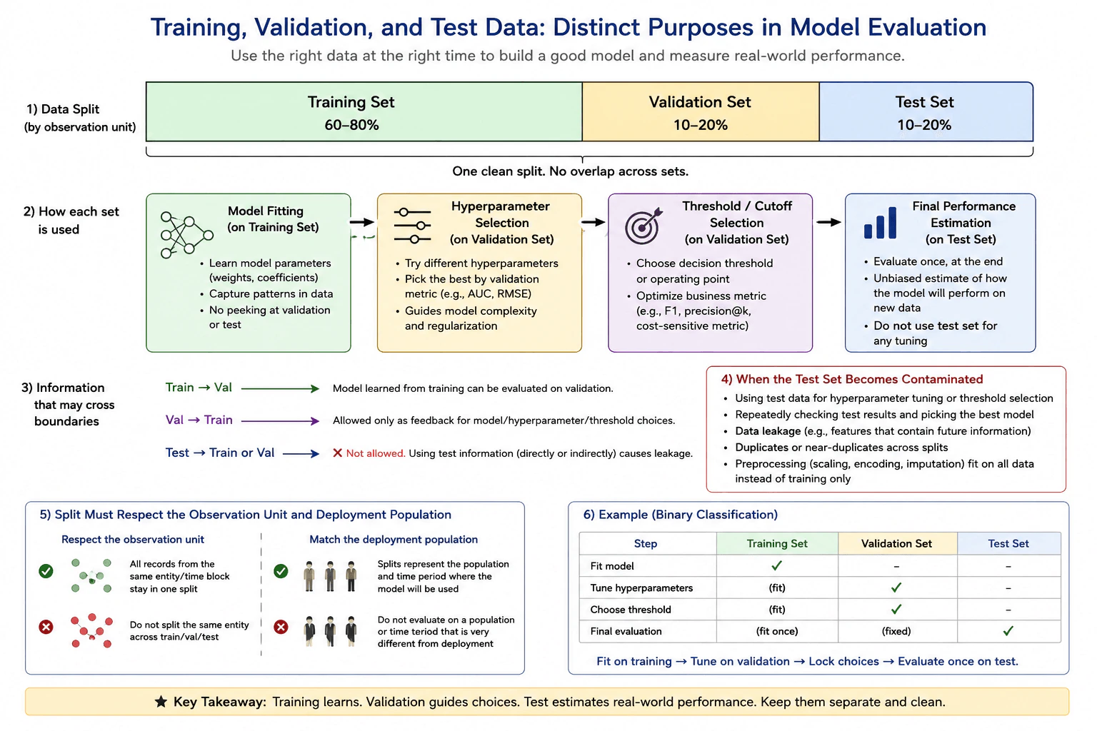
What are the distinct purposes of training, validation, and test data? diagram
How to Explain It in an Interview

Start with the training set. Its purpose is learning. The fitting algorithm uses training examples to estimate model parameters, such as weights or coefficients, and capture patterns in the data. Any preprocessing step that learns values from data, such as scaling, encoding, imputation, or feature selection, must also be fitted using only allowed training data. The learned transformation can then be applied to validation and test data without refitting it there.

Next use the validation set for development choices. A model fitted on training data can generate predictions on validation data. Those results can guide hyperparameter selection, model complexity, regularization, feature or model choices, and decision-threshold selection. For example, candidate models may be compared with an appropriate validation metric. The diagram gives examples such as AUC or RMSE. For a thresholded classifier, the validation set can also be used to choose an operating point with a metric such as F1, precision at a required level, or another cost-sensitive criterion when that criterion matches the problem.

Validation information is therefore allowed to flow back into the development process as feedback. If validation results cause me to change hyperparameters, regularization, features, the model, or the threshold, that is expected. Because those choices were influenced by validation data, validation performance is not an untouched final estimate.

The test set has a different purpose. After training and validation-based choices are complete, I lock the preprocessing, features, model settings, and threshold. I then evaluate that fixed pipeline on the test set. If the test set has remained untouched and represents deployment, its result is the final estimate of how the chosen model should perform on new data from that setting. I should not use the test result for additional tuning and still describe a later score on the same test set as an untouched estimate.

A test set becomes contaminated when test information influences development. Examples include tuning hyperparameters using test performance, selecting the threshold after seeing test scores, repeatedly checking test results and choosing the best model, using test information for feature selection, or fitting preprocessing such as scaling, encoding, or imputation on all data before evaluation. Duplicates or near-duplicates across splits can also leak information and make performance look better than it really is.

The split must respect the observation unit. If several records belong to the same entity or time block and are not independent for the intended prediction problem, those records should stay in one split instead of being divided across training, validation, and test data. Otherwise the model may be evaluated on observations that are too closely related to data it already saw.

The split must also match the intended deployment population. The validation and test data should represent the population and time period where the model will be used. If the real task is future-facing, preserving time order may be more appropriate than a random split. Evaluating on a very different population or time period can produce a number that does not answer the real deployment question.

The diagram shows example proportions of roughly 60–80% training and 10–20% each for validation and test. These percentages are examples, not universal rules. The important sequence is: fit on training, tune and select on validation, lock the choices, and then evaluate once on the untouched test set.

Technical Approach
  1. Define the observation unit and the intended deployment population and time period.
  2. Create non-overlapping training, validation, and test splits so related observations do not improperly cross boundaries.
  3. Fit learned preprocessing and model parameters using training data only.
  4. Apply the fitted pipeline to validation data and use validation feedback to choose hyperparameters, model complexity, features when appropriate, regularization, and the decision threshold.
  5. Repeat training and validation as needed without using test results.
  6. Lock the preprocessing, features, hyperparameters, fitted model procedure, and threshold.
  7. Evaluate the finalized model on the untouched test set for the final performance estimate.
  8. If test results influence another development decision, treat that test set as contaminated for final evaluation and use a new independent test set for a clean final estimate.
Practical Insights

Keeping separate validation and test sets means fewer observations are available for model fitting. With a small dataset, that can make estimates noisier, so a careful validation method such as cross-validation may help during development while an independent final test set is still protected. Repeated tuning can also overfit to validation data. Group-aware or time-aware splitting may leave less convenient sample sizes than a random split, but it is necessary when it better matches the observation unit or deployment setting. The main tradeoff is using less data for fitting in exchange for a more trustworthy evaluation.

Why Interviewers Ask This

Interviewers want to know whether you understand why training, validation, and test data must have separate roles. They are testing whether you can fit a model, tune it without leaking information, keep the final test set independent, select thresholds correctly, and construct splits that respect observation units, time, and the intended deployment population. These choices determine whether the reported final performance is a trustworthy estimate for new data.

Common interview mistakes

Common mistakes include fitting the model with validation or test data, tuning hyperparameters from test performance, choosing a threshold after seeing test results, repeatedly checking the test set and reporting the best run, fitting preprocessing on the full dataset before evaluation, allowing duplicate or closely related records from the same observation unit to cross splits, ignoring time order for a future-facing deployment, and evaluating on a population that does not represent intended deployment. Another mistake is treating example split percentages such as 60–80% training and 10–20% validation and test as mandatory rules.

Interview tip

Start with the simple rule: training learns, validation guides choices, and test estimates final performance. Then explain the boundary: validation feedback may influence development, but test information must not. Finish by mentioning observation-unit integrity, deployment population, time boundaries, and preprocessing leakage because these are common ways an apparently clean split becomes invalid.
Interviewer may ask next
What if several rows belong to the same customer or another repeated entity?

If those rows are not independent for the intended prediction problem, keep all related records from that observation unit in the same split. Putting some records from one entity in training and closely related records from the same entity in test can leak information and make test performance too optimistic. The split should therefore be performed at the appropriate group or entity level. If time also matters, the grouping rule and temporal ordering should both reflect how predictions will be made in deployment.

What should you do if you see the test result, change the model, and then evaluate on the same test set again?

The test set has now influenced model development, so it is contaminated as an untouched final evaluation set. I can use what I learned from it during further development, but I should not treat another score on that same set as a clean final estimate. After the new choices are finalized and locked, I need a new independent test set that has not influenced those choices and that represents the intended deployment population.

32. How would you choose a baseline before evaluating a model?Model Evaluation And ValidationEasy

Question Details

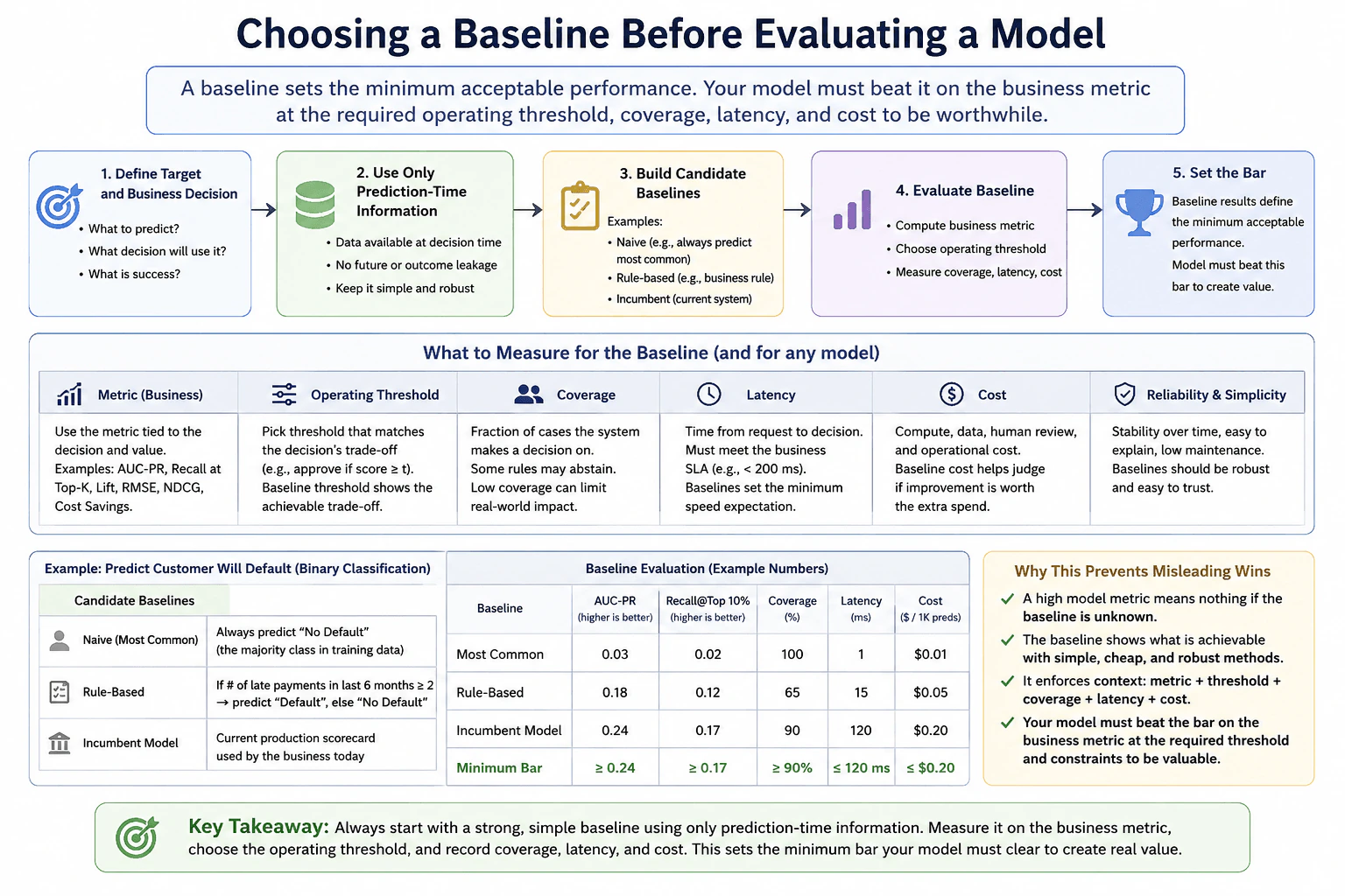
Given a prediction target and a business decision, define at least one naive, rule-based, or incumbent baseline that uses only prediction-time information. Explain how the baseline metric, operating threshold, coverage, latency, and cost establish the minimum acceptable performance and prevent an impressive-looking model metric from being evaluated without context.

Short Interview Answer (30-60 seconds)

I would choose a simple baseline that uses only prediction-time information, such as the majority class, a business rule, or the incumbent system. I would measure its business metric, operating threshold, coverage, latency, and cost. That becomes the minimum practical bar the new model must beat.

Detailed Explanation

I first define what we are predicting and which business decision will use that prediction. Then I choose at least one realistic baseline that can run using only information available at prediction time. It could be a naive majority-class rule, a simple business rule, or the incumbent production system. I evaluate that baseline using the same business metric and operating conditions planned for the new model. I record its threshold, coverage, latency, cost, reliability, and simplicity. These results create the minimum practical bar for deciding whether the new model adds value.

Useful Questions to Ask the Interviewer
  1. What prediction target are we trying to estimate, and what business decision will use it?
  2. Which prediction errors are most costly for that decision?
  3. Is there an existing rule or production model that already makes this decision?
  4. Which metric should define success for the business decision?
  5. What operating constraints matter, such as required coverage, maximum latency, or maximum cost?
How would you choose a baseline before evaluating a model? diagram
How to Explain It in an Interview

First, define the prediction target and the business decision. A baseline is useful only if it represents a realistic alternative to the new model.

The approved example is a binary customer-default prediction problem. The system predicts whether a customer will default, and the comparison is made against simple alternatives that the business could actually use.

Next, restrict every baseline to information that exists when the prediction is made. Future outcomes must not be used. This prevents leakage and keeps the baseline realistic.

I would normally consider three baseline types. A naive baseline can always predict the most common class. In the example, it always predicts "No Default." A rule-based baseline can apply a simple business rule. The example predicts "Default" when the number of late payments in the last six months is at least two; otherwise it predicts "No Default." An incumbent baseline is the current production scorecard already used by the business.

Then I evaluate each baseline in the same way I plan to evaluate the new model. The business metric measures predictive value for the decision. The operating threshold defines when a score or rule turns into an action. Coverage is the fraction of cases for which the system can make the intended decision. Latency is the time from request to decision. Cost includes compute, data, human review, and operational expense. Reliability and simplicity also matter because a stable, explainable baseline may be cheaper to operate and easier to trust.

The diagram shows the comparison clearly. The most-common baseline has AUC-PR 0.03, Recall@Top 10% of 0.02, 100% coverage, 1 ms latency, and a cost of $0.01 per 1,000 predictions. The rule-based baseline has AUC-PR 0.18, Recall@Top 10% of 0.12, 65% coverage, 15 ms latency, and a cost of $0.05 per 1,000 predictions. The incumbent model has AUC-PR 0.24, Recall@Top 10% of 0.17, 90% coverage, 120 ms latency, and a cost of $0.20 per 1,000 predictions.

In this example, the incumbent is the strongest practical baseline. The diagram therefore shows a minimum bar of AUC-PR at least 0.24, Recall@Top 10% at least 0.17, coverage at least 90%, latency no more than 120 ms, and cost no more than $0.20 per 1,000 predictions. The operating threshold itself should be chosen to match the business tradeoff, such as the acceptable balance between false positives and false negatives.

The new model should not be accepted just because one offline metric looks impressive. It should beat the relevant baseline by a meaningful amount on the business metric while still satisfying the required threshold behavior, coverage, latency, and cost constraints. Otherwise, the apparent improvement may not create real business value.

This baseline also prevents misleading comparisons. A new model can look strong if it is compared only with a deliberately weak naive rule, even when an incumbent system already performs much better. Comparing against the strongest realistic alternative gives the model metric proper context.

The main limitation is that a baseline is not a permanent universal target. Business rules, costs, traffic, and incumbent systems can change. I would document how the baseline was defined and re-evaluate it when the operating environment changes.

Technical Approach
  1. Define the prediction target and the business decision that will use it.
  2. List the information available at prediction time and exclude future or outcome information.
  3. Define realistic baseline candidates: a naive baseline, a simple rule-based baseline, and the incumbent system when one exists.
  4. Evaluate each baseline with the business-relevant metric.
  5. Choose the operating threshold or rule cutoff that matches the business decision and error tradeoff.
  6. Record coverage, latency, operational cost, reliability, and simplicity.
  7. Identify the strongest relevant practical baseline instead of choosing only the easiest baseline to beat.
  8. Use that baseline to establish the minimum acceptable predictive and operational performance.
  9. Compare the new model and baseline under the same prediction-time information and comparable operating conditions.
Practical Insights

A naive baseline is usually very cheap, fast, and easy to maintain, but it may have weak predictive value. A rule-based baseline is still simple and explainable, but its coverage or predictive quality may be limited. An incumbent model may be slower or more expensive, but it represents the value the business already receives. A new model is worthwhile only when its extra predictive value justifies any extra latency, compute, data, operational work, and maintenance. Coverage matters too, because a strong metric on only a small fraction of cases may provide less value than a slightly weaker method that can handle most cases.

Why Interviewers Ask This

Interviewers want to see whether I can evaluate a model in context instead of treating one model metric as meaningful by itself. A strong answer shows that I understand realistic baselines, prediction-time information, leakage prevention, business-aligned metrics, operating thresholds, coverage, latency, cost, reliability, simplicity, and fair comparison with an existing system.

Common interview mistakes

Common mistakes are evaluating the new model without defining a baseline, using a deliberately weak baseline even when a stronger incumbent exists, allowing future or outcome information into the baseline, comparing systems under different operating conditions, ignoring the operating threshold, and forgetting coverage, latency, cost, reliability, or simplicity. Another mistake is assuming that a higher offline metric automatically means more business value. A model can score better and still be a poor replacement if it is too slow, too expensive, unstable, or unable to cover enough cases.

Interview tip

Start with the business decision, then name the realistic baseline candidates. Say explicitly that they use only prediction-time information. Finish by explaining that the business metric, operating threshold, coverage, latency, and cost together define the practical bar the new model must clear.

Interviewer may ask next
What if the naive baseline is easy to beat, but an incumbent production model already performs much better?

I would not use the weak naive baseline as the only acceptance bar. I can still report it for context, but the incumbent system is the more important practical comparison. In the diagram, the naive baseline has AUC-PR 0.03 while the incumbent has AUC-PR 0.24. Merely beating 0.03 would therefore not show that the new model improves the current system. I would compare the new model with the incumbent and require a meaningful improvement on the business metric while still satisfying the required operating threshold behavior, coverage, latency, and cost constraints.

What if the new model has a better predictive metric than the baseline but has worse latency or higher cost?

I would treat that as a business tradeoff instead of automatically accepting the model. In the diagram, the incumbent baseline provides 90% coverage, 120 ms latency, and a cost of $0.20 per 1,000 predictions. A new model with a better predictive metric may still be unacceptable if it violates required latency or cost limits. If those constraints are hard requirements, the model should not be adopted until it meets them. If they are flexible, I would compare the added business value with the additional operational cost before making the decision.

33. How do you interpret a binary classifier's confusion matrix?Model Evaluation And ValidationEasy

Question Details

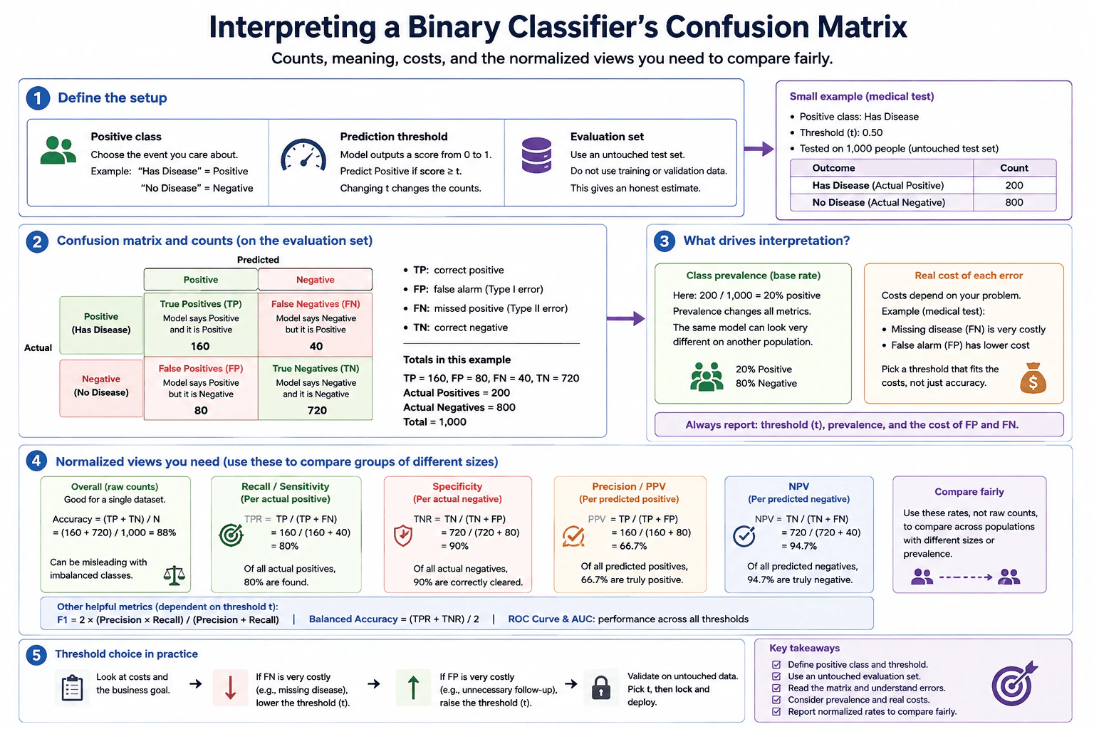
Define the positive class, prediction threshold, and counts of true positives, false positives, true negatives, and false negatives on an untouched evaluation set. Explain how class prevalence and the real cost of each error affect interpretation, and show which normalized views are needed when comparing populations of different sizes.

Short Interview Answer (30-60 seconds)

I first define the positive class and the prediction threshold. Then I read TP, FP, TN, and FN on an untouched evaluation set. I interpret those counts using class prevalence and the real cost of each error. For fair comparisons across populations, I use normalized rates such as recall, specificity, precision, and NPV.

Detailed Explanation

A confusion matrix compares a binary classifier's predicted class with the actual class. Before reading it, define which class is positive and state the prediction threshold. Then calculate the four counts on an untouched evaluation set: true positives, false positives, false negatives, and true negatives. The counts show what kinds of decisions the model made, but they need context. Class prevalence affects how common each outcome is, while false positives and false negatives may have different real costs. For populations of different sizes, normalized rates are more informative than raw counts alone.

Useful Questions to Ask the Interviewer
  1. Which outcome should be treated as the positive class?
  2. Is the prediction threshold already fixed, or should I discuss how changing it affects the errors?
  3. Which error is more costly in this problem: a false positive or a false negative?
  4. Are we comparing populations with different sizes or different positive-class prevalence?
How do you interpret a binary classifier's confusion matrix? diagram
How to Explain It in an Interview

Start with the setup. In the diagram's example, the positive class is "Has Disease" and the negative class is "No Disease." The classifier outputs a score from 0 to 1. With threshold t = 0.50, a score at or above 0.50 is predicted positive. Changing t changes how many cases are predicted positive, so it also changes TP, FP, FN, and TN.

The confusion matrix should be reported on an untouched evaluation set. This data should not have been used to train the model or repeatedly tune its threshold. That gives a more honest estimate of performance after the model and threshold are fixed.

The example has 1,000 evaluation cases. There are 200 actual positives and 800 actual negatives. The matrix contains TP = 160, FP = 80, FN = 40, and TN = 720.

A true positive, or TP, is a case that is actually positive and predicted positive. Here, 160 people with the disease are correctly predicted positive.

A false positive, or FP, is actually negative but predicted positive. Here, 80 people without the disease are incorrectly flagged positive. This is a false alarm.

A false negative, or FN, is actually positive but predicted negative. Here, 40 people with the disease are missed.

A true negative, or TN, is actually negative and predicted negative. Here, 720 people without the disease are correctly predicted negative.

The totals provide a useful check. Actual positives equal TP + FN = 160 + 40 = 200. Actual negatives equal TN + FP = 720 + 80 = 800. All four cells add to 1,000.

Next consider class prevalence, also called the base rate. It is the fraction of the population that is actually positive. In this example, prevalence is 200 / 1,000 = 20%. Prevalence matters because a classifier can produce different raw counts and different predictive values when used in a population with a different positive-class rate. Therefore, raw counts from two populations should not be compared without considering their sizes and prevalence.

Then consider the real cost of each error. The two errors do not have to be equally bad. In this medical-test example, missing a disease is a false negative and may be much more costly than creating a false alarm. If false negatives are very costly, a lower threshold can be considered. A lower threshold normally predicts more cases as positive, which tends to reduce false negatives and increase recall, but it can also increase false positives. If false positives are more costly, a higher threshold can be considered. This normally predicts fewer positives and can reduce false positives, but it can create more false negatives. The threshold should therefore reflect the real decision tradeoff, not accuracy alone.

Normalized rates make the matrix easier to interpret and make comparisons across different population sizes more meaningful.

Recall, also called sensitivity or true positive rate, normalizes within the actual positive class. Recall = TP / (TP + FN). In the example, recall = 160 / (160 + 40) = 80%. It answers: of all actual positives, what fraction did the model find? The complementary false-negative rate is FN / (TP + FN), which is 20% here.

Specificity, also called true negative rate, normalizes within the actual negative class. Specificity = TN / (TN + FP). Here, specificity = 720 / (720 + 80) = 90%. It answers: of all actual negatives, what fraction did the model correctly identify as negative? The complementary false-positive rate is FP / (FP + TN), which is 10% here.

Precision, also called positive predictive value or PPV, normalizes within predicted positives. Precision = TP / (TP + FP). Here, precision = 160 / (160 + 80) = about 66.7%. It answers: of all cases predicted positive, what fraction are actually positive?

Negative predictive value, or NPV, normalizes within predicted negatives. NPV = TN / (TN + FN). Here, NPV = 720 / (720 + 40) = about 94.7%. It answers: of all cases predicted negative, what fraction are actually negative?

These normalized views answer different questions. Row normalization by actual class gives rates such as recall, false-negative rate, specificity, and false-positive rate. Prediction-based normalization gives values such as precision and NPV. Normalizing every cell by the total population gives each outcome as a share of all cases. That can describe the overall population composition, but it does not remove the effect of prevalence.

Accuracy is (TP + TN) / N. In this example, accuracy = (160 + 720) / 1,000 = 88%. Accuracy can be useful, but it can be misleading when one class is much more common than the other. Balanced accuracy gives equal weight to the two actual classes and is (TPR + TNR) / 2. F1 combines precision and recall when that tradeoff is useful. ROC-AUC summarizes ranking performance across thresholds, while the confusion matrix describes behavior at one particular threshold.

When comparing populations of different sizes, do not compare only TP, FP, FN, and TN counts. Compare appropriate normalized rates. If prevalence also differs, remember that recall and specificity are conditioned on the actual class, while precision and NPV can change as prevalence changes. Report prevalence together with the rates so the comparison has the correct context.

A strong interpretation therefore states the positive class, threshold, evaluation set, TP, FP, FN, TN, prevalence, important normalized rates, and the relative cost of FP and FN. If the threshold still needs to be selected, use separate threshold-selection data or another valid validation procedure to choose it. Then lock the threshold and measure the final result on untouched evaluation data.

Technical Approach
  1. Define the positive and negative classes.
  2. State the prediction threshold.
  3. Use an untouched evaluation set after the model and threshold are fixed.
  4. Count TP, FP, FN, and TN by comparing predictions with actual labels.
  5. Check that TP + FN equals actual positives, TN + FP equals actual negatives, and all four cells equal the total.
  6. Calculate class prevalence.
  7. Calculate normalized rates such as recall, specificity, precision, and NPV.
  8. Interpret FP and FN using their real-world costs.
  9. When comparing populations of different sizes, compare normalized rates rather than raw counts alone.
  10. If threshold selection is still required, choose the threshold before final evaluation using the relevant error-cost tradeoff.
Practical Insights

The computation is simple because each evaluation example contributes to exactly one of four cells. The main difficulty is choosing the right interpretation. Raw counts depend on population size. Prevalence changes the mix of positive and negative cases and strongly affects predictive values such as precision and NPV. Accuracy may hide poor performance on a minority class. Lowering or raising the threshold trades false negatives against false positives, so the useful threshold depends on their real costs. Final performance should be measured only after that choice is fixed.

Why Interviewers Ask This

Interviewers want to know whether you can turn four confusion-matrix counts into useful model judgment. You should define the positive class and prediction threshold, correctly distinguish TP, FP, TN, and FN, and interpret them on untouched evaluation data. You should also understand why prevalence matters, why false positives and false negatives may have different real costs, and why normalized rates are more useful than raw counts when populations have different sizes.

Common interview mistakes

Common mistakes include not defining which class is positive, forgetting that the confusion matrix depends on the prediction threshold, mixing up false positives and false negatives, evaluating on data used for training or repeated tuning, comparing raw counts across populations of different sizes, ignoring prevalence, and relying only on accuracy when classes are imbalanced. Another mistake is treating recall, specificity, precision, and NPV as interchangeable. They use different denominators and answer different questions. It is also a mistake to change the threshold after inspecting the final untouched evaluation results and then report those same results as an unbiased final estimate.

Interview tip

Start by drawing the 2-by-2 matrix with actual and predicted classes clearly labeled. Define TP, FP, FN, and TN in plain English before giving formulas. Then explain prevalence, the different costs of FP and FN, and the normalized rates needed for fair comparison. This shows both mathematical understanding and practical model judgment.

Interviewer may ask next
What if the positive class becomes much rarer in another population?

I would not compare only the raw confusion-matrix counts because the population size and prevalence have changed. I would report the new prevalence and compare normalized rates. Recall and specificity describe performance within the actual positive and negative classes. Precision and NPV describe the reliability of positive and negative predictions, but they can change when prevalence changes. So even if sensitivity and specificity stay similar, precision may become lower when positives are rarer. The interpretation should therefore include both the normalized rates and the new base rate.

How would you change the threshold if false negatives became much more costly than false positives?

I would generally consider lowering the prediction threshold so more cases are predicted positive. That tends to reduce false negatives and increase recall, but it can also increase false positives and reduce specificity or precision. I would compare candidate thresholds using the relative cost of FN and FP on appropriate threshold-selection data, choose the tradeoff that matches the decision goal, lock that threshold, and then report final performance on untouched evaluation data.

34. How do precision, recall, and F1 score differ?Model Evaluation And ValidationEasy

Question Details

For a binary classifier with a specified positive class and threshold, define precision, recall, and F1 from confusion-matrix counts. Explain what happens when a denominator is zero, why F1 ignores true negatives, how prevalence affects precision, and which metric matters when false-positive and false-negative costs differ.

Short Interview Answer (30-60 seconds)

Precision asks, "Of the predicted positives, how many were correct?" Recall asks, "Of the actual positives, how many did we find?" F1 is their harmonic mean. Emphasize precision when false positives are costly, recall when false negatives are costly, and use F1 when one score should balance both.

Detailed Explanation

For a binary classifier, first choose the positive class and fix the decision threshold. The confusion matrix then gives true positives (TP), false positives (FP), false negatives (FN), and true negatives (TN). Precision measures how trustworthy positive predictions are. Recall measures how completely the classifier finds actual positives. F1 combines precision and recall into one score. These three metrics do not use TN. Their values can change when the threshold changes, and precision can also change when the positive-class prevalence changes.

Useful Questions to Ask the Interviewer
  1. Which class should I treat as the positive class?
  2. Is the decision threshold already fixed, or should metric choice help determine it?
  3. Are false positives or false negatives more costly?
  4. Is the positive class rare in the population?
  5. Do you want precision and recall separately, or one combined score such as F1?
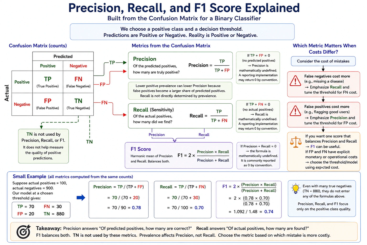
How do precision, recall, and F1 score differ? diagram
How to Explain It in an Interview

Start with the confusion matrix. TP means the model predicted positive and the example was actually positive. FP means the model predicted positive but the example was actually negative. FN means the model predicted negative but the example was actually positive. TN means the model predicted negative and the example was actually negative.

Precision is TP / (TP + FP). It answers: "Among everything the model predicted as positive, what fraction was actually positive?" High precision means fewer false alarms among positive predictions. If TP + FP = 0, the classifier predicted no positives, so the mathematical ratio is undefined. A reporting implementation may return 0 by convention, so that convention should be stated.

Recall, also called sensitivity, is TP / (TP + FN). It answers: "Among all actual positives, what fraction did the model find?" High recall means fewer missed positives. If TP + FN = 0, there are no actual positives, so the mathematical ratio is undefined. A reporting implementation may also return 0 by convention.

F1 is 2 × Precision × Recall / (Precision + Recall). When the component quantities are defined, it is equivalent to 2TP / (2TP + FP + FN). F1 is a harmonic mean, so it is high only when both precision and recall are reasonably high. If Precision + Recall = 0, the displayed precision-recall formula has a zero denominator and is mathematically undefined; it is commonly reported as 0 by convention.

F1 ignores true negatives because neither precision nor recall contains TN, and the equivalent count-based F1 formula contains only TP, FP, and FN. This is useful when positive-class performance is the main concern, but it also means F1 does not tell us how well the classifier handles the negative class.

Prevalence means the fraction of examples that are actually positive. Precision can depend strongly on prevalence. For example, if the true-positive rate and false-positive rate stay the same but positives become rarer, false positives can make up a larger share of predicted positives, so precision falls. Recall is conditioned on actual positives, so prevalence does not directly determine recall.

Using the diagram's example, TP = 70, FP = 20, FN = 30, and TN = 880. Precision = 70 / (70 + 20) = 70 / 90 = 0.78. Recall = 70 / (70 + 30) = 70 / 100 = 0.70. F1 = 2 × (0.78 × 0.70) / (0.78 + 0.70) ≈ 0.74. The TN count of 880 does not enter any of these formulas.

Metric choice should follow the cost of mistakes. If false negatives are more costly, emphasize recall and tune the threshold with false-negative cost in mind. If false positives are more costly, emphasize precision and tune the threshold with false-positive cost in mind. If you want one score that balances precision and recall, F1 can be useful. If false positives and false negatives have explicit monetary or operational costs, choose the model or threshold using expected cost rather than assuming F1 represents those costs.

Finally, the decision threshold matters. Changing it changes which examples are predicted positive or negative, which changes TP, FP, FN, and TN. Precision, recall, and F1 can therefore change with the threshold. The best metric and threshold depend on the real decision objective and the relative consequences of the two error types.

Technical Approach
  1. Specify the positive class and decision threshold.
  2. Count TP, FP, FN, and TN from the confusion matrix.
  3. Compute Precision = TP / (TP + FP) when the denominator is nonzero.
  4. Compute Recall = TP / (TP + FN) when the denominator is nonzero.
  5. Compute F1 = 2 × Precision × Recall / (Precision + Recall) when that denominator is nonzero.
  6. State the reporting convention used for undefined zero-denominator cases.
  7. Consider positive-class prevalence because it can materially affect precision.
  8. Choose the metric and threshold according to false-positive and false-negative costs; when explicit costs are known, compare choices using expected cost.
Practical Insights

The arithmetic is very cheap because the metrics use only confusion-matrix counts. The important tradeoff is statistical and operational, not computational. Changing the threshold usually changes the balance between false positives and false negatives, so precision and recall often move in different directions. F1 summarizes both but ignores true negatives. Precision can also change when prevalence changes. If false-positive and false-negative errors have different real costs, a single metric may not represent the decision correctly.

Why Interviewers Ask This

Interviewers want to see whether the candidate understands what precision, recall, and F1 measure, can derive them from confusion-matrix counts, handles zero-denominator edge cases correctly, understands why true negatives are excluded, recognizes how prevalence can affect precision, and chooses metrics based on the relative cost of false positives and false negatives.

Common interview mistakes

Common mistakes are swapping precision and recall, using FN in the precision denominator, using FP in the recall denominator, claiming that F1 uses true negatives, saying F1 is automatically the best metric for imbalanced data, ignoring zero-denominator cases, comparing precision across populations without considering prevalence, treating metric choice as independent of the threshold, and choosing F1 when explicit false-positive and false-negative costs should drive the decision.

Interview tip

Start with the confusion matrix and the two simple questions answered by precision and recall. Then define F1. Finish with zero denominators, why TN is excluded, prevalence, threshold effects, and error costs. This shows both formula knowledge and practical evaluation judgment.

Interviewer may ask next
What happens if the classifier predicts no positive examples?

Then TP + FP = 0, so precision is mathematically undefined because its denominator is zero. A reporting implementation may return 0 by convention, but that convention should be stated. If actual positives still exist, TP = 0 and recall is 0. With precision and recall both reported as 0, F1 is commonly reported as 0 by convention.

If false negatives become much more expensive than false positives, should I still optimize F1?

Not automatically. F1 balances precision and recall but does not encode the actual cost of false positives and false negatives. If false negatives are much more expensive, I would emphasize recall and tune the threshold to reduce false negatives. If the costs are explicitly known, I would choose the model or threshold using expected cost while still reporting precision, recall, and F1 for interpretation.

35. When is area under the precision-recall curve preferable to ROC AUC?Model Evaluation And ValidationMedium

Question Details

Consider a rare-positive classifier whose scores will be used to rank cases for limited review capacity. Define the positive class, prevalence, precision-recall curve, average precision or area convention, and ROC AUC. Explain how each responds to many true negatives and why the relevant recall and precision region, not a single global number, should drive acceptance.

Short Interview Answer (30-60 seconds)

I prefer PR-based evaluation when positives are rare and false positives among top-ranked cases matter, especially with limited review capacity. Many true negatives can keep ROC false-positive rates small. I would report AP or AUPRC with its convention, then inspect precision and recall in the operating region we will actually use.

Detailed Explanation

For a rare-positive classifier, the model gives each case a score and ranks cases from highest to lowest. The positive class is the outcome of interest, Y = 1, and prevalence, π = P(Y = 1), is the share of cases that are positive. If only a limited number of cases can be reviewed, the practical question is how many true positives appear among those reviewed cases without too many false positives. Precision-recall evaluation exposes this directly, while ROC AUC can understate the operational false-positive burden when true negatives are very numerous.

Useful Questions to Ask the Interviewer
  1. How rare is the positive class, or what is its expected prevalence?
  2. Is the model mainly used to rank cases for a fixed review capacity, or must we choose a threshold for another operational constraint?
  3. Which matters more in the review region: higher recall, higher precision, or a specific error-cost tradeoff?
  4. Should the reported PR summary use average precision or another stated area-under-the-PR-curve convention?
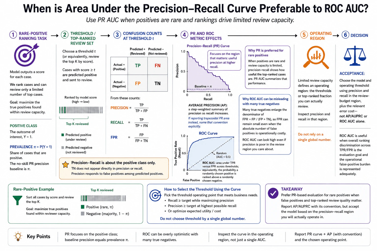
When is area under the precision-recall curve preferable to ROC AUC? diagram
How to Explain It in an Interview

Start with the task. The classifier produces a score for each case. We rank cases by score and can review only a limited top-ranked set. The positive class is Y = 1. Prevalence is π = P(Y = 1), the fraction of all cases that are positive.

Choose a threshold t, or equivalently review the top K cases. Cases with score at or above the threshold are selected for review. At that operating point, the confusion counts are true positives, false positives, false negatives, and true negatives.

Precision is TP / (TP + FP). It answers: among the cases selected for review, what fraction are actually positive? Recall is TP / (TP + FN). It answers: among all real positives, what fraction did we find? False-positive rate is FP / (FP + TN).

A precision-recall curve plots precision against recall as the threshold changes. For a random-ranking baseline, expected precision equals the prevalence π. A useful global summary is average precision, or AP, which is a step-weighted summary of precision as recall increases. If a different PR-area convention, such as trapezoidal integration, is reported, I would name that convention explicitly rather than treat every PR-area calculation as identical to AP.

ROC AUC summarizes the area under true-positive rate versus false-positive rate across thresholds. It also has a ranking interpretation: apart from the usual treatment of ties, it is the probability that a randomly chosen positive receives a higher score than a randomly chosen negative.

The key difference appears when negatives are abundant. In FPR = FP / (FP + TN), many true negatives make the denominator large. FPR can therefore remain small even when the absolute number of false positives is operationally costly. True negatives do not appear directly in precision or recall. Precision instead responds directly to false positives among selected cases, which is often what matters when reviewers have limited capacity.

That does not mean AP or AUPRC alone should decide whether the model is accepted. Limited review capacity defines an operating region: the thresholds or top-ranked fraction that can actually be reviewed. I would inspect precision and recall specifically in that region. If the review budget permits only the top K cases, I care about the precision among those reviewed cases and the corresponding recall, not performance at thresholds that will never be used.

ROC AUC is still useful when overall ranking discrimination across TPR and FPR is the evaluation goal and the operational false-positive burden is adequately represented. The problem is treating ROC AUC as sufficient when the real decision depends on rare positives, scarce review capacity, and false positives among selected cases.

For acceptance, I would compare candidate models in the actual review-budget region and choose an operating threshold using the required precision, recall, and relevant error cost. I would report the PR curve and AP or AUPRC with its convention, but I would not accept a model solely because one global PR AUC or ROC AUC number is higher.

Technical Approach
  1. Define the positive class Y = 1 and its prevalence π = P(Y = 1).
  2. Confirm that model scores rank cases and identify the available review capacity.
  3. Translate that capacity into a threshold t or top-K operating region.
  4. At relevant thresholds, compute TP, FP, FN, and TN.
  5. Compute precision = TP / (TP + FP), recall = TP / (TP + FN), and FPR = FP / (FP + TN).
  6. Plot the precision-recall curve and state the summary convention, such as average precision.
  7. Use ROC AUC as a complementary measure of overall ranking discrimination rather than the only acceptance criterion.
  8. Inspect precision and recall in the actual review-budget region.
  9. Choose the model and operating threshold using that region and the relevant error-cost tradeoff.
Practical Insights

The main tradeoff is interpretation, not computational cost. PR metrics make false positives among selected cases visible and are often more informative when positives are rare. ROC AUC gives a broad ranking summary, but many true negatives can make the false-positive rate look small even when the absolute false-positive count is expensive. AP or AUPRC is also a global summary and can hide weak performance in the exact part of the curve that will be used. The practical work is therefore choosing and validating the correct operating region instead of relying on one convenient number.

Why Interviewers Ask This

Interviewers want to see whether you can choose an evaluation metric based on prevalence, ranking goals, review capacity, false-positive cost, and the actual operating region. They also want you to understand why ROC AUC can look strong in a rare-positive problem with many true negatives, how precision-recall metrics respond differently, and why a global summary metric should not replace threshold- and capacity-based judgment.

Common interview mistakes

Common mistakes are saying PR AUC is always better for imbalanced data; treating class balance alone as the rule for choosing ROC AUC; forgetting that the random-ranking PR precision baseline equals prevalence; confusing precision with false-positive rate; saying true negatives directly affect precision or recall; treating average precision and every PR-area integration convention as identical; assuming a high ROC AUC guarantees acceptable precision in a rare-positive review setting; and accepting a model from AP, AUPRC, or ROC AUC without checking the precision-recall operating region that matches the actual review budget.

Interview tip

Start with the operational goal: rare positives, ranked scores, and limited review capacity. Then write the formulas for precision, recall, and FPR. Use the large true-negative denominator in FPR to explain why ROC AUC can look strong. Finish by saying acceptance should come from precision and recall in the operating region, not from one global AUC.

Interviewer may ask next
What if the positive class is still rare, but the review team only cares about the first small fraction of the ranked list?

Then the local operating region becomes even more important. I would evaluate the thresholds or top-ranked fraction that correspond to that review capacity and report the precision achieved there together with the resulting recall. AP or AUPRC can still summarize the overall precision-recall curve, but it includes regions the team may never use. I would therefore compare models primarily on performance inside the feasible review region and use the global summary as supporting information.

What if one model has higher ROC AUC but another has better precision in the review-budget region?

If limited review capacity and false-positive burden define the real objective, I would generally prefer the model with better precision-recall behavior in that operating region, assuming its recall and error-cost tradeoff satisfy the requirement. The higher-ROC-AUC model may discriminate better on average across all thresholds, but that does not guarantee better performance where the system will actually operate. I would report both results and make the acceptance decision from the relevant operating region.

36. How do explained variance and R-squared differ?Model Evaluation And ValidationMedium

Question Details

For continuous targets with observed values and predictions on a fixed evaluation set, define both metrics and the reference mean used by R-squared. Compare their treatment of systematic prediction bias, possible value ranges, and interpretation. Include a concrete error pattern where one metric looks better than the other and explain which better matches the business loss.

Short Interview Answer (30-60 seconds)

Explained variance measures how much variability the predictions capture, while R-squared measures squared-error improvement over predicting the observed-target mean. A constant prediction bias can leave explained variance unchanged but reduce R-squared. So when squared-error accuracy and systematic bias matter, R-squared is usually more informative.

Detailed Explanation

Both metrics evaluate continuous predictions on the same fixed evaluation set, but they answer slightly different questions. Explained variance asks how much target variability remains after accounting for the variability of the residuals. R-squared asks how much squared error the model removes compared with always predicting the mean of the observed targets. Their main difference appears with systematic bias. If every prediction is shifted by a constant amount, explained variance may still look perfect, while R-squared decreases because the absolute errors become larger. This distinction matters when choosing a metric that reflects business loss.

Useful Questions to Ask the Interviewer
  1. Is the main business concern capturing relative variation, or must predictions also be accurate in their absolute level?
  2. Does the business loss penalize squared errors, or does it use another error cost such as absolute error?
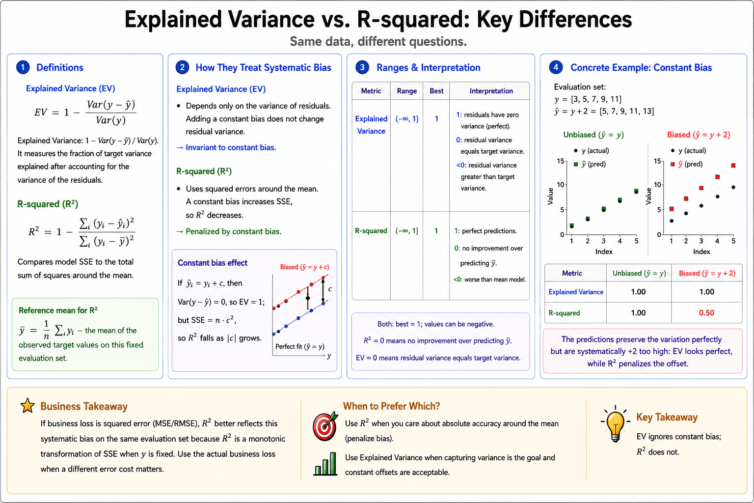
How do explained variance and R-squared differ? diagram
How to Explain It in an Interview

Start with the common setup. We have observed continuous targets yᵢ and predictions ŷᵢ on one fixed evaluation set.

Explained variance is EV = 1 - Var(y - ŷ) / Var(y). It compares the variance of the residuals, y - ŷ, with the variance of the observed targets. EV = 1 means the residuals have zero variance. EV = 0 means residual variance equals target variance. EV can be negative when residual variance is larger than target variance.

R-squared is R² = 1 - Σ(yᵢ - ŷᵢ)² / Σ(yᵢ - ȳ)², where ȳ = (1/n)Σyᵢ is the mean of the observed target values on that same evaluation set. The denominator is the squared error of the constant baseline that predicts ȳ for every observation. R² = 1 means perfect predictions. R² = 0 means the model provides no squared-error improvement over that mean baseline. R² can be negative when the model is worse than predicting the mean.

The important distinction is systematic prediction bias. Suppose ŷᵢ = yᵢ + c for every observation. Then every residual equals -c, so Var(y - ŷ) = 0 and explained variance equals 1, assuming Var(y) > 0. However, the squared-error numerator for R² is n·c², so R² decreases as the size of the constant offset increases. Explained variance therefore ignores a constant level shift, while R² penalizes it.

Use the diagram's concrete example: y = [3, 5, 7, 9, 11]. With perfect predictions ŷ = y, both EV and R² equal 1.00. Now shift every prediction by +2: ŷ = [5, 7, 9, 11, 13]. The residual is always -2, so its variance is zero and EV remains 1.00. For R², SSE = 5 × 2² = 20. The target mean is 7, and Σ(yᵢ - 7)² = 40. Therefore R² = 1 - 20/40 = 0.50.

The model has captured the pattern of variation perfectly, so EV looks excellent, but every prediction is systematically too high. If the business loss is squared error, such as MSE or RMSE, R² better reflects this problem because, for a fixed nonconstant target set, R² is a monotonic transformation of SSE. If the business uses a different loss, evaluate that loss directly rather than assuming either metric perfectly represents business impact.

Technical Approach
  1. Compute residuals eᵢ = yᵢ - ŷᵢ on the fixed evaluation set.
  2. For explained variance, compare Var(e) with Var(y): EV = 1 - Var(e) / Var(y).
  3. Compute the observed-target mean ȳ = (1/n)Σyᵢ.
  4. For R-squared, compare model SSE with the mean-baseline total sum of squares: R² = 1 - Σeᵢ² / Σ(yᵢ - ȳ)².
  5. Inspect whether residuals have a nonzero mean or another systematic offset. A constant offset can leave EV unchanged while lowering R².
  6. Match the metric to the business objective. If squared error is the loss, R² has the same ordering as SSE on the same fixed nonconstant target set; otherwise inspect the actual business loss directly.
Practical Insights

Both metrics are inexpensive to compute. Their calculation grows linearly with the number of observations and can be done from simple running summaries. The important tradeoff is statistical, not computational. Explained variance can hide a constant bias because it depends on residual variance. R-squared penalizes that bias through squared errors and compares the model with the mean-prediction baseline. Neither metric should replace the actual business loss when the cost of errors follows a different rule.

Why Interviewers Ask This

Interviewers want to see whether you understand that two regression metrics that look similar can reward different prediction behavior. The key judgment is recognizing that explained variance focuses on residual variability, while R-squared evaluates squared error relative to the observed-target mean baseline. A strong answer also connects systematic prediction bias to the business loss instead of choosing a metric only because its score looks higher.

Common interview mistakes

Common mistakes are saying that explained variance and R-squared are always equivalent, forgetting that R-squared uses the mean of the observed targets as its reference baseline, or assuming a high explained-variance score guarantees unbiased predictions. Another mistake is saying EV = 0 specifically means the model predicts the mean; it only means residual variance equals target variance. Candidates also sometimes claim that either score must lie between 0 and 1, even though both can be negative for nonconstant targets. Finally, do not treat R-squared as a universal business metric: its close alignment here is specifically with squared-error loss on the same fixed target set.

Interview tip

Lead with the bias distinction: explained variance can stay perfect under a constant offset, while R-squared falls. Then define the observed-target mean baseline for R-squared and use the +2 example to make the difference concrete. Finish by tying metric choice to the actual business loss.

Interviewer may ask next
Why does adding the same constant to every prediction leave explained variance unchanged?

If ŷᵢ = yᵢ + c, every residual is yᵢ - ŷᵢ = -c. A constant sequence has zero variance, so Var(y - ŷ) =

  1. For a nonconstant target, EV = 1 - 0 / Var(y) =
  2. This does not mean the predictions are numerically correct; it means the residuals have no variability. R-squared still sees the error because each residual contributes c² to SSE.
If the business cares about absolute error instead of squared error, should you still prefer R-squared over explained variance?

Not as the final business metric. R-squared is based on squared residuals, so it aligns naturally with squared-error objectives on the same fixed target set. If the business cost is absolute error, evaluate MAE or the actual business loss directly. The explained-variance-versus-R-squared comparison is still useful diagnostically because it can reveal systematic bias, but neither should replace the metric that represents the real error cost.

37. How would you choose a classification threshold when error costs are asymmetric?Model Evaluation And ValidationHard

Question Details

A calibrated score predicts a harmful event; missing one event costs much more than reviewing a false alert, and review capacity is limited. Define the evaluation population, cost matrix or utility, capacity constraint, and candidate thresholds. Estimate expected cost with uncertainty, examine calibration and subgroup behavior, compare with the current policy, and specify an acceptance rule robust to prevalence change.

Short Interview Answer (30-60 seconds)

I would choose the feasible threshold that minimizes expected decision cost, not default to 0.5 or optimize a generic metric. I would enforce the review-capacity limit, quantify uncertainty, check calibration and subgroup behavior, compare with the current policy, and verify robustness to plausible prevalence changes.

Detailed Explanation

A calibrated score estimates the probability of a harmful event. The goal is not to maximize accuracy, F1, or another generic classification metric. Missing a harmful event costs much more than reviewing a false alert, but only a limited number of cases can be reviewed. I would therefore define the evaluation population, decision costs, and review budget first. Then I would evaluate candidate thresholds on validation data, choose the lowest-cost feasible threshold, quantify uncertainty, inspect calibration and subgroup behavior, compare it with the current policy, and test whether the decision remains acceptable under plausible prevalence changes.

Useful Questions to Ask the Interviewer
  1. What population will receive scores and decisions in production?
  2. What is the unit of one prediction or review decision, and what exactly defines the harmful event?
  3. What are the costs or utilities for a missed event, a false alert, a reviewed true event, and a correct non-review decision?
  4. Is review capacity a hard maximum number of cases K, a maximum review rate r, or both?
  5. What current threshold or policy should the new rule be compared against?
  6. Which subgroups are important to evaluate separately?
  7. What prevalence range should the policy remain robust to?
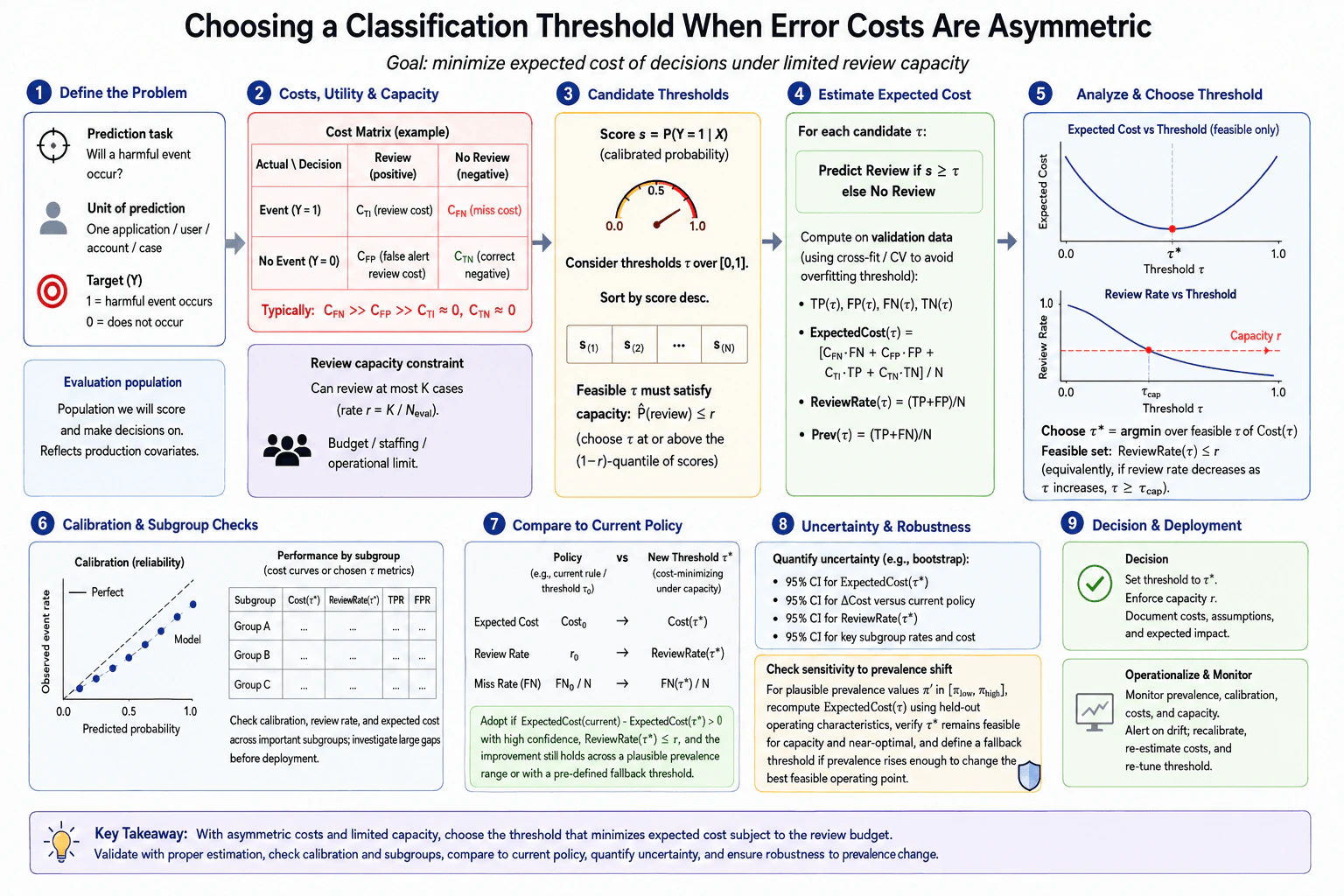
How would you choose a classification threshold when error costs are asymmetric? diagram
How to Explain It in an Interview

First, I would define the evaluation population so it reflects the population on which the policy will actually make decisions. The score is s = P(Y=1 | X), where Y=1 means the harmful event occurs and Y=0 means it does not. A threshold τ creates the decision rule: review when s ≥ τ and do not review otherwise.

Next, I would define the decision cost matrix before choosing a threshold. Let C_FN be the cost of missing a harmful event, C_FP the cost of reviewing a false alert, C_TI the cost of reviewing a true event, and C_TN the cost of a correct non-review decision. The important asymmetry is that C_FN is much larger than C_FP. The actual values should come from the real operational decision process, not from an arbitrary model metric.

I would then translate review capacity into a constraint. If at most K of N evaluation cases can be reviewed, the maximum review rate is r = K/N. For threshold τ:

ReviewRate(τ) = [TP(τ) + FP(τ)] / N.

A threshold is feasible only when ReviewRate(τ) ≤ r. Because review rate normally decreases as τ increases, the feasible region is at or above the capacity threshold τ_cap when that monotonic relationship holds.

Next, I would generate candidate thresholds from the calibrated score distribution, such as the unique observed score values over [0,1]. Sorting scores from highest to lowest makes it easy to evaluate how the confusion-matrix counts change as the cutoff moves.

For every candidate threshold, I would compute TP(τ), FP(τ), FN(τ), and TN(τ) on threshold-selection validation data. The expected decision cost per evaluated case is:

ExpectedCost(τ) = [C_FN·FN(τ) + C_FP·FP(τ) + C_TI·TP(τ) + C_TN·TN(τ)] / N.

The selected threshold is:

τ* = argmin over feasible τ of ExpectedCost(τ),

subject to:

ReviewRate(τ) ≤ r.

This is the central decision rule. A lower threshold usually catches more harmful events but creates more reviews and false alerts. A higher threshold reduces review load but can create more expensive misses. The correct operating point balances those costs while respecting the hard capacity constraint.

I would estimate uncertainty instead of treating the validation estimate as exact. For example, I could use bootstrap resampling or an appropriate cross-validation procedure to estimate 95% confidence intervals for ExpectedCost(τ*), the cost improvement versus the current policy, ReviewRate(τ*), and important subgroup rates and costs. Threshold selection should remain inside the allowed validation procedure. I would not repeatedly tune the threshold on an untouched final test set.

Because the score is described as calibrated, I would still verify calibration on held-out evaluation data. A reliability plot compares predicted probabilities with observed event rates. If the probabilities are materially miscalibrated, I would recalibrate using data that is separate from the final policy evaluation and then repeat threshold selection because recalibration can change the numerical score scale.

I would also evaluate important subgroups at τ*. For each subgroup, I would inspect calibration, review rate, expected cost, TPR, and FPR. Large differences may show that a single global threshold works poorly for one cohort. I would investigate those gaps before deployment rather than assuming one threshold automatically satisfies every fairness objective.

Next, I would compare the proposed threshold with the current policy on the same evaluation population. I would compare expected cost, review rate, and miss rate, together with uncertainty. Define:

ΔCost = ExpectedCost(current) - ExpectedCost(τ*).

A positive ΔCost means the proposed threshold has lower expected cost.

I would then test robustness to prevalence change. For plausible prevalence values π' in [π_low, π_high], I would recompute expected cost using held-out operating characteristics. Under the explicit assumption that the conditional TPR and FPR remain approximately stable:

ExpectedCost(τ; π') = π'·[C_FN·(1-TPR(τ)) + C_TI·TPR(τ)] + (1-π')·[C_FP·FPR(τ) + C_TN·(1-FPR(τ))].

The corresponding expected review rate is:

ReviewRate(τ; π') = π'·TPR(τ) + (1-π')·FPR(τ).

I would verify that τ* remains feasible for capacity and near-optimal across the plausible prevalence range. If prevalence can rise enough to change the best feasible operating point, I would define a fallback or re-thresholding rule in advance. If calibration, TPR, or FPR also drift, prevalence adjustment alone is not sufficient and the policy must be revalidated.

My production acceptance rule would be: adopt τ* only if ExpectedCost(current) - ExpectedCost(τ*) > 0 with high confidence, ReviewRate(τ*) ≤ r, and the improvement still holds across the plausible prevalence range or a predefined fallback threshold is available.

After deployment, I would monitor prevalence, calibration, realized costs when labels arrive, subgroup behavior, and review capacity. If drift makes the threshold no longer feasible or cost-effective, I would alert, recalibrate when appropriate, re-estimate costs, re-threshold, or roll back to the approved fallback policy.

Technical Approach
  1. Define the production-like evaluation population, prediction unit, harmful-event target, and current policy.
  2. Define the complete decision cost or utility matrix, especially the high false-negative cost.
  3. Convert review capacity into r = K/N when at most K of N cases can be reviewed.
  4. Generate candidate thresholds from the calibrated scores over [0,1].
  5. On threshold-selection validation data, compute TP, FP, FN, TN, review rate, and expected cost for every candidate threshold.
  6. Remove thresholds with ReviewRate(τ) > r.
  7. Choose τ* as the feasible threshold with minimum expected cost.
  8. Estimate uncertainty for ExpectedCost(τ*), ΔCost versus the current policy, ReviewRate(τ*), and important subgroup rates and costs.
  9. Check calibration and subgroup behavior at τ*.
  10. Compare τ* with the current policy on the same evaluation population.
  11. Recompute expected cost and review rate across plausible prevalence values, explicitly stating the assumptions used for the shift analysis.
  12. Accept the new threshold only when the cost improvement is supported by uncertainty, capacity is satisfied, and prevalence robustness is acceptable or a fallback threshold is predefined.
  13. Monitor prevalence, calibration, realized costs, subgroup behavior, and capacity after deployment, with re-thresholding or rollback when assumptions fail.
Practical Insights

The main tradeoff is between costly missed harmful events and cheaper false alerts. Lowering the threshold normally catches more harmful events but creates more reviews and can exceed capacity. Raising it reduces review load but may create more expensive misses. Computationally, threshold evaluation is usually inexpensive once validation scores are available. The harder work is statistical and operational: estimating credible error costs, getting enough labeled data for useful confidence intervals, checking calibration and important subgroups, and maintaining the policy when prevalence or model behavior changes.

Why Interviewers Ask This

This question tests whether a Data Scientist can convert calibrated probability scores into defensible operating decisions when error types have unequal consequences and operational capacity is limited. It checks cost-sensitive threshold selection, validation design, uncertainty estimation, calibration, subgroup evaluation, comparison with an existing policy, robustness to prevalence changes, and production judgment. A strong answer separates model discrimination from probability calibration and from the final thresholded business decision.

Common interview mistakes

Common mistakes are using 0.5 by default; optimizing accuracy, F1, AUROC, or another generic metric instead of decision cost; ignoring the review-capacity constraint; using an incomplete or unjustified cost matrix; selecting the threshold repeatedly on the final test set; reporting only a point estimate without uncertainty; assuming calibration remains valid after distribution shift; ignoring subgroup calibration, review rate, and cost differences; comparing the current and proposed policies on different populations; and running a prevalence-shift calculation without stating the assumption that the relevant conditional operating characteristics remain stable.

Interview tip

Start with the decision objective, not a model metric. State the asymmetric costs and capacity constraint, write the feasible expected-cost optimization, then explain uncertainty, calibration, subgroup checks, comparison with the current policy, prevalence robustness, and the production acceptance rule.

Interviewer may ask next
What would you do if the model ranks cases well but the probability scores are not well calibrated?

I would separate ranking quality from probability quality. A model can rank cases correctly while its probability values are systematically too high or too low. I would fit a calibration method using data that is separate from the final policy evaluation, verify the new calibration on held-out data, and then repeat threshold selection using the recalibrated scores. I would not keep the old numerical threshold automatically because recalibration can change the score scale. I would again evaluate expected cost, capacity, uncertainty, subgroup behavior, and the comparison with the current policy.

What if prevalence rises after deployment and the selected threshold would exceed review capacity?

I would treat capacity as a hard constraint rather than keep the old threshold automatically. Under a prevalence-only shift assumption, I would recompute ReviewRate(τ; π') = π'·TPR(τ) + (1-π')·FPR(τ) and expected cost across candidate thresholds, then choose the lowest-cost threshold that remains feasible. If a fallback threshold was predefined, I could activate it immediately. If calibration, TPR, or FPR are also changing, I would not rely on prevalence adjustment alone; I would revalidate or recalibrate the policy and roll back if the approved acceptance conditions are no longer met.

38. How would you evaluate and improve probability calibration?Model Evaluation And ValidationHard

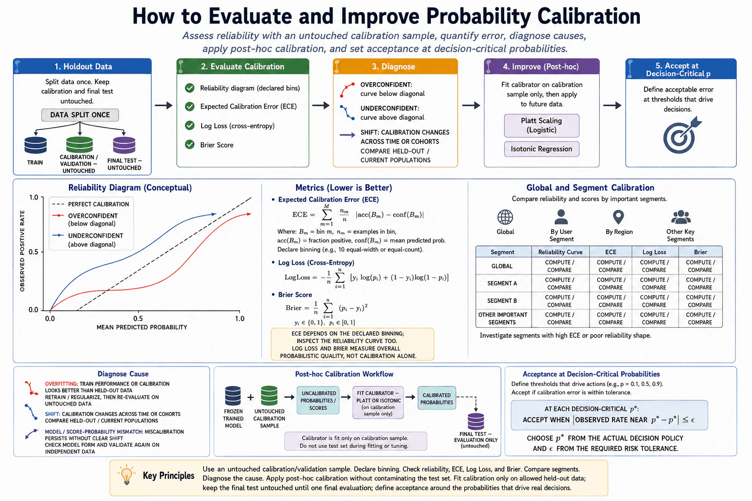
Question Details

For a probabilistic classifier, use an untouched calibration or validation sample to assess reliability diagrams, expected calibration error with declared binning, log loss, and Brier score. Compare global and segment calibration, identify whether shift or overfitting is involved, evaluate post-hoc calibration without contaminating the test set, and define acceptance at decision-critical probabilities.

Short Interview Answer (30-60 seconds)

I would use an untouched calibration or validation sample to inspect a reliability diagram and measure ECE with declared bins, log loss, and Brier score globally and by segment. I would diagnose overfitting or shift, fit Platt scaling or isotonic regression only on allowed held-out data, then evaluate the frozen pipeline once on the untouched final test set.

Detailed Explanation

Probability calibration asks whether predicted probabilities match observed frequencies. If a classifier assigns many cases a probability near 0.7, about 70% of comparable cases should be positive. I would evaluate this on an untouched calibration or validation sample, not on the training data or final test set. I would inspect a reliability diagram and calculate ECE with explicitly declared bins, log loss, and Brier score. I would compare global and segment behavior, diagnose overfitting or distribution shift, test post-hoc calibration, and define acceptance around the probabilities that drive real decisions.

Useful Questions to Ask the Interviewer
  1. Which predicted probabilities are decision-critical, and what calibration error is acceptable around them?
  2. Do we already have a separate calibration or validation sample and an untouched final test set?
  3. Which cohorts or segments are important enough to evaluate separately?
  4. Should the validation population match current production conditions, or are there known shifts we should test?
How would you evaluate and improve probability calibration? diagram
How to Explain It in an Interview

First, separate the data roles. Train the classifier using only the training data. Keep a calibration or validation sample untouched by model fitting. Keep the final test set separate and untouched until the final evaluation. If I use post-hoc calibration, I fit the calibrator only on the allowed calibration data and never use the final test set to choose the calibration method or tune its parameters.

Next, inspect a reliability diagram. The x-axis is mean predicted probability and the y-axis is observed positive rate. Perfect calibration lies on the diagonal. If the curve is below the diagonal, predicted probabilities are higher than observed frequencies, so the model is overconfident. If the curve is above the diagonal, the model is underconfident.

Then quantify probability quality. Expected Calibration Error, or ECE, divides predictions into declared probability bins and computes a weighted average of the absolute gap between each bin's mean predicted probability and observed positive rate. I would always report how the bins were constructed because ECE depends on the binning scheme. I would inspect the reliability curve as well instead of treating one ECE value as a complete description of calibration.

I would also calculate log loss and Brier score. Lower values are better for both. Log loss strongly penalizes confident wrong predictions. Brier score is the mean squared difference between predicted probability and the binary outcome. These are overall probabilistic-quality measures, not calibration-only measures, so they complement rather than replace the reliability diagram and ECE.

I would run the same checks globally and for important segments. A model can appear calibrated overall while being poorly calibrated for a particular cohort. For each important segment, I would compare the reliability curve, ECE, log loss, and Brier score. I would also examine uncertainty around these estimates when sample sizes are limited, because a small segment can produce a noisy reliability curve or unstable metric.

If calibration is poor, I would diagnose the cause before applying a correction. Overfitting is plausible when training performance or calibration looks substantially better than held-out behavior. In that case, I would consider retraining or stronger regularization and then evaluate again on untouched held-out data. Distribution shift is plausible when calibration changes across time, cohorts, or populations, so I would compare held-out and current populations. Persistent miscalibration without clear shift can also indicate a mismatch between model scores and true probabilities.

For post-hoc improvement, I would freeze the trained classifier and generate its uncalibrated probabilities or scores on the untouched calibration sample. I could fit Platt scaling, which applies a parametric logistic mapping, or isotonic regression, which learns a more flexible monotonic mapping. Platt scaling is smoother and can work better with limited calibration data. Isotonic regression is more flexible but can overfit when the calibration sample is small.

After calibration, I would recompute the reliability diagram and the same probability metrics on permitted held-out data. I would also check important segments and the decision-critical probability regions. Once the model and calibrator are selected and frozen, I would use the untouched final test set once for an unbiased final evaluation.

Acceptance should focus on probabilities that actually drive decisions. For each decision-critical probability p*, I would define a tolerance epsilon based on the required risk tolerance and accept calibration when |observed rate near p* - p*| <= epsilon. The exact p* values and tolerances should come from the real decision policy rather than being invented during evaluation.

The main tradeoff is statistical precision. More bins can reveal local calibration problems but leave fewer observations in each bin. Fewer bins are more stable but can hide local errors. Segment analysis has the same issue. I would therefore interpret calibration using the reliability shape, declared-bin ECE, log loss, Brier score, segment behavior, uncertainty, and the decision-critical regions together rather than relying on one aggregate number.

Technical Approach
  1. Split the data so training, calibration or validation, and final test roles remain separate.
  2. Train the classifier using only allowed training data and freeze it before calibration evaluation.
  3. Generate probabilities or scores on the untouched calibration or validation sample.
  4. Plot a reliability diagram with mean predicted probability on the x-axis and observed positive rate on the y-axis.
  5. Declare the binning strategy and calculate ECE using those bins.
  6. Calculate log loss and Brier score as complementary overall probability-quality metrics.
  7. Repeat the reliability and metric checks globally and for important segments, and examine uncertainty when sample sizes are limited.
  8. Diagnose whether poor calibration is associated with overfitting, population shift, or a persistent score-to-probability mismatch.
  9. If appropriate, fit Platt scaling or isotonic regression using only allowed calibration data.
  10. Re-evaluate the calibrated probabilities on permitted held-out data using the same diagnostics.
  11. Freeze the model-plus-calibrator pipeline and use the final test set once for unbiased final evaluation.
  12. Define acceptance around decision-critical probabilities using tolerances derived from the actual decision policy and required risk tolerance.
Practical Insights

The calculations are usually inexpensive compared with training the classifier because they operate on stored probabilities and labels. The larger cost is statistical. Reliable calibration estimates need enough examples, especially inside individual probability bins and segments. More bins give finer detail but fewer observations per bin. Fewer bins are more stable but can hide local problems. Platt scaling is simple and smooth and generally needs less calibration data. Isotonic regression is more flexible but can overfit with a small calibration sample. Reserving calibration and final test data also leaves less data for training, but it protects the credibility of the evaluation.

Why Interviewers Ask This

This question tests whether a candidate can evaluate the quality of predicted probabilities rather than only classification accuracy. It checks understanding of leakage-safe data splits, reliability diagrams, calibration metrics, cohort analysis, uncertainty, distribution shift, post-hoc calibration, and how to translate calibration quality into decision-specific acceptance criteria without tuning on the final test set.

Common interview mistakes

Common mistakes include calibrating on the final test set, repeatedly choosing calibration methods using test results, reporting ECE without declaring the binning scheme, treating log loss or Brier score as calibration-only metrics, checking only global calibration and missing poorly calibrated segments, assuming a particular reliability-curve shape proves distribution shift, applying post-hoc calibration without investigating overfitting or population change, ignoring uncertainty in small bins or segments, and inventing acceptance thresholds that are not tied to actual decisions.

Interview tip

Present the answer as a leakage-safe sequence: separate the data, inspect reliability, quantify it, compare segments, diagnose the cause, calibrate only on allowed held-out data, re-evaluate, and reserve the final test set for one unbiased evaluation. End by connecting acceptance to decision-critical probabilities.

Interviewer may ask next
What would you do if the global reliability diagram looks good but one important segment is badly miscalibrated?

I would not accept the global result as sufficient. I would first check whether the segment has enough observations for a stable estimate and examine its reliability curve, ECE, log loss, Brier score, and uncertainty. Then I would investigate whether that segment differs from the broader population because of shift, different base rates, or model misspecification. I would address that cause before assuming calibration alone is sufficient. If I considered a segment-specific calibrator, it would still require independent calibration data and leakage-safe validation.

How would you choose between Platt scaling and isotonic regression?

I would compare them using only allowed calibration or validation data, never the final test set. Platt scaling uses a smooth parametric logistic mapping and is attractive when calibration data is limited or the correction is relatively simple. Isotonic regression is non-parametric and can represent a more flexible monotonic relationship, but it can overfit with small samples. I would compare their held-out reliability curves, ECE, log loss, Brier score, segment behavior, and performance around decision-critical probabilities, then freeze the selected method before final test evaluation.

39. What is a machine learning system, and which components take a model from data to production?Machine Learning System DesignEasy

Question Details

Define a production machine learning system beyond the trained model. Walk through data collection, validation, feature preparation, training, evaluation, versioning, deployment, batch or online inference, monitoring, feedback, and retraining, and explain the interfaces and failure modes that connect these components.

Short Interview Answer (30-60 seconds)

A machine learning system is the complete pipeline around the model. It collects and validates data, prepares features, trains and evaluates a model, versions approved artifacts, deploys them for batch or online prediction, monitors production behavior, and feeds new labels back into retraining.

Detailed Explanation

A production machine learning system is more than a trained model. It is a connected lifecycle that turns raw data into predictions and then learns from production outcomes. Data must be checked before training, features must be prepared consistently, and a model must pass evaluation before deployment. The system also needs versioning so we know which data, code, configuration, model, and evaluation results produced a release. After deployment, predictions may be generated through online serving or batch inference. Monitoring checks operational and model-related signals, while feedback supplies new labels for future retraining.

Useful Questions to Ask the Interviewer
  1. Do we need online predictions, batch predictions, or both?
  2. How quickly do true outcomes or labels become available after a prediction?
  3. Which evaluation, fairness, business, and service checks decide whether a model can be deployed?
  4. What rollout and rollback behavior is expected if a new model performs badly?
  5. Are there important security, privacy, governance, or cost constraints across the lifecycle?
What is a machine learning system, and which components take a model from data to production? diagram
How to Explain It in an Interview

Start with the main idea: the model is only one component. A production ML system is an end-to-end data and prediction pipeline with a feedback loop.

  1. Data collection. Raw information can come from databases, applications, sensors, logs, clickstreams, or third-party APIs. The system needs a clear data interface so downstream stages receive the expected fields and formats.
  1. Data validation and quality. Check the schema, missing values, outliers, duplicates, and consistency before using the data. Critical quality failures should stop the pipeline instead of silently creating a bad training set. Duplicate, missing, or invalid records can distort learning, and schema changes can break later stages.
  1. Feature engineering and preparation. Clean and transform the validated data. Typical operations include scaling, bucketing, encoding, and aggregation. A feature store can hold reusable feature definitions for offline training and online serving. The same feature meaning should be preserved between training and production to avoid training-serving skew. Historical features should use only information that was available at the prediction time, otherwise future information can leak into training.
  1. Model training. Train a selected algorithm using the prepared data. Hyperparameter tuning and cross-validation can be used when useful. Training may run on CPU or GPU compute. The important production requirement is reproducibility: the training result should be traceable to known data, feature logic, code, parameters, and configuration.
  1. Evaluation and validation. Never deploy only because a training metric looks good. Evaluate the model on appropriate held-out data. Depending on the task, metrics may include accuracy, AUC, or RMSE. Perform error analysis and relevant bias or fairness checks. A pass/fail validation gate should decide whether the candidate model can move forward. Leakage is a major failure mode because it can make evaluation look much better than real production performance.
  1. Versioning and registry. Store the approved model with a model version and its lineage. Track the related code, data, features, parameters, metrics, and other metadata needed for reproducibility. This makes it possible to understand what produced the deployed model and to return to a known previous version if necessary.
  1. Deployment. Package the approved model and release it to production. A staged strategy such as canary or blue-green rollout reduces risk because the new version can be observed before it fully replaces the old version. The system should also keep a rollback path to a known working version if the release causes serious problems.
  1. Inference. A deployed model can support online serving, batch inference, or both. Online serving handles an application request and returns a prediction in the request path. Batch inference processes many records offline and writes predictions for later use. These modes have different latency, reliability, and cost tradeoffs. For online serving, end-to-end latency includes more than model execution; request handling, feature access, networking, and surrounding service work also matter.
  1. Monitoring and observability. Monitor several kinds of signals separately. Service monitoring covers latency, throughput, errors, logs, traces, and general service health. Data-quality monitoring checks whether incoming inputs remain valid. Drift monitoring can detect changes in input distributions or prediction distributions. Model-quality monitoring uses true outcomes when labels become available. Drift is a warning signal, not automatic proof that quality has declined. Alerts should expose failures instead of allowing silent breakage.
  1. Feedback and retraining. Production outcomes and new labels must be joined back to the correct earlier predictions at the correct entity and time. Labels may arrive immediately or after a delay, so model-quality measurement can lag behind service monitoring. The new labeled data can update the training set and trigger retraining or fine-tuning when justified. A newly trained model should still pass evaluation and versioning before deployment; retraining should not mean automatic promotion.

The approved diagram includes a churn-prediction example. In that example, user activity is input data, churn in the next 30 days is a binary target, features include items such as login count, average session time, last ticket age, plan type, and monthly charges, and XGBoost is an example model. AUC-ROC and Precision@K are shown as example metrics. These details illustrate the pipeline; they are not universal requirements for every machine learning system.

Several concerns apply across all stages. Security covers access control, authentication, and encryption. Privacy and compliance govern how data is handled. Governance and audit controls track policies and approvals. Cost management covers compute and storage. Documentation and runbooks explain how the system is operated and recovered.

Common failure modes connect directly to the lifecycle. Bad data can create a bad model. Data or concept drift can reduce performance. Leakage can produce overly optimistic metrics. Serving bugs can create wrong predictions. Latency and timeouts can hurt the user experience even if the model is statistically good. Delayed feedback can leave the model stale. A mature ML system detects these problems, keeps lineage, supports safe deployment and rollback, and closes the feedback loop.

Technical Approach
  1. Clarify whether inference is online, batch, or both, and understand how labels become available.
  2. Collect data through a clear source interface.
  3. Validate schema, missing values, duplicates, outliers, and consistency, and stop on critical invalid data.
  4. Prepare reusable features and keep offline and online feature logic consistent.
  5. Train the model with reproducible data, code, parameters, and configuration.
  6. Evaluate it on held-out data, perform error analysis and relevant fairness checks, and apply a pass/fail deployment gate.
  7. Version the model and its supporting lineage in a registry.
  8. Deploy gradually with a strategy such as canary or blue-green and keep rollback available.
  9. Run online or batch inference according to the product need.
  10. Monitor service health, data quality, drift, model quality, and relevant outcomes separately.
  11. Join later outcomes to the correct predictions, update training data, retrain when justified, and repeat evaluation before promotion.
Practical Complexity & Trade-offs

The important tradeoffs are system complexity, latency, reliability, compute cost, storage cost, and maintenance effort. Online inference gives fast predictions but needs an always-available serving path and stricter latency monitoring. Batch inference is usually simpler when predictions can wait, but results are less immediate. More validation, monitoring, versioning, and staged deployment add engineering work, but they reduce silent failures and make diagnosis and rollback easier. A feature store can reduce duplicated feature logic but adds another system to operate. Frequent retraining can react faster to new data, but it costs more compute and can promote noise if evaluation gates are weak.

Where it is used

This design is useful whenever a model must run repeatedly outside an experiment or notebook. Examples include classification, ranking, recommendation, forecasting, anomaly detection, risk scoring, and other systems that must keep producing predictions from changing production data. The same lifecycle applies whether inference is delivered through an online API, scheduled batch jobs, or both.

Why Interviewers Ask This

Interviewers want to see whether you understand that production machine learning is more than model training. They are testing whether you can connect data quality, feature preparation, training, evaluation, versioning, deployment, inference, monitoring, feedback, and retraining into one end-to-end system. They also want you to recognize important failure modes such as bad data, leakage, drift, serving bugs, latency problems, delayed feedback, and unsafe deployment.

Common interview mistakes

Common mistakes are treating the trained model as the whole system; skipping schema and data-quality validation; allowing training-serving feature skew; using future information and causing leakage; deploying based only on a training metric; failing to version the model and its lineage; confusing online serving with batch inference; monitoring only model metrics while ignoring latency, errors, and service health; treating drift as proof that quality declined; losing the connection between a prediction and its later outcome; retraining without re-evaluation; and deploying a new version without staged rollout or rollback.

Interview tip

Explain the system as one loop: data -> validation -> features -> training -> evaluation -> registry -> deployment -> inference -> monitoring -> feedback -> retraining. As you move through it, mention the interface and one important failure mode at each stage. Emphasize that validation gates, monitoring, versioning, lineage, and feedback are what turn a trained model into a production ML system.

Interviewer may ask next
What changes if the true label arrives days or weeks after the prediction?

Service monitoring can still happen immediately, but model-quality monitoring must wait for the delayed outcome. Store enough information to connect each later outcome to the correct earlier prediction and model version. Before labels arrive, monitor data quality, input or prediction drift, latency, throughput, errors, logs, and other service signals, but do not treat those signals as proof that model quality changed. When the labels become available, join them at the correct entity and time, calculate the relevant model and business metrics, update the training data, and retrain only when the chosen trigger or review process justifies it. The new model must pass evaluation again before deployment.

How would you choose between online inference and batch inference, and what should happen if online serving fails?

Use online inference when an application needs a prediction as part of an interactive request. Use batch inference when predictions can be computed periodically for many records and consumed later. Online serving has stricter latency and reliability requirements and usually requires more operational work. Batch inference is simpler when immediate answers are unnecessary. The exact fallback for online failure depends on the product requirement, so it should be clarified instead of invented. Possible designs include using a known previous model, a cached or precomputed result, a non-ML default, or returning an explicit failure. Whatever fallback is chosen should be observable, and a bad model release should be able to roll back to a known working version.

40. Design orchestration for versioned machine-learning data workflows.Machine Learning System DesignEasy

Question Details

A workflow is a DAG whose tasks ingest, transform, validate, and atomically publish datasets used for training. Define workflow, run, task-attempt, artifact, and lineage states; scheduling across heterogeneous compute pools; leases, retries, idempotency, cancellation, backfills, validation gates, quarantine, and publication. Connect data versions to feature and label generation, training jobs, model registry entries, downstream batch or online serving, feedback and retraining, data-quality and drift signals, access control, secret handling, tenant fairness, observability, disaster recovery, and cost.

Short Interview Answer (30-60 seconds)

I would use a versioned DAG controlled by a scheduler and state store. Tasks get leases, run idempotently on appropriate compute pools, write staged artifacts, pass validation gates, and publish through an atomic version commit. Versioned lineage then connects approved data to training, model registration, batch or online serving, feedback, monitoring, backfills, and retraining.

Detailed Explanation

The goal is to make every machine-learning dataset build reproducible, retry-safe, and traceable. I would represent ingestion, transformation, validation, feature generation, label generation, and publication as a versioned DAG. A control plane stores workflow and run state, schedules task attempts onto appropriate compute pools, manages leases, and records events. Tasks write staged, versioned artifacts instead of changing published data in place. Validation decides whether a version is atomically committed or quarantined. Published versions then feed training, model registration, batch inference, online serving, feedback analysis, monitoring, and retraining.

Useful Questions to Ask the Interviewer
  1. Which task types need CPU, GPU, serverless, data-engine, or large batch compute?
  2. Which validation failures should automatically quarantine a version, and can an operator ever approve a blocked version?
  3. Should backfills target a time range, selected data versions, or both?
  4. Which consumers need published versions: training jobs, batch inference, online serving, or all of them?
  5. What access-control, tenant-isolation, disaster-recovery, observability, and cost requirements are most important?
Design orchestration for versioned machine-learning data workflows. diagram
How to Explain It in an Interview
1. Start with explicit state models

A workflow is the versioned DAG definition plus dependencies and policy. Its lifecycle can be ACTIVE, PAUSED, or DEPRECATED.

A run is one execution of a workflow for a chosen parameter set, time range, or data-version range. Its normal state path is QUEUED to RUNNING and then SUCCEEDED, FAILED, or CANCELLED.

A task attempt is one try to execute one task. Its successful path is PENDING to LEASED to RUNNING to SUCCEEDED. FAILED and CANCELLED are terminal outcomes for that attempt. A retry creates a new task attempt rather than changing a failed attempt back into a running one.

An artifact is a versioned output such as raw data, processed data, features, labels, metadata, schemas, or a quality report. Its lifecycle is STAGED to VALIDATED to PUBLISHED, or QUARANTINED when validation fails.

Lineage is the graph connecting versioned inputs to outputs. It can be provisional while a run is executing and becomes committed lineage when the corresponding artifact version is successfully published.

2. Separate orchestration from execution

The control plane owns the workflow registry, scheduler, state store, lease service, event handling, policy, and orchestration decisions. Workers execute the actual tasks. This separation lets one workflow use several execution environments without putting scheduling logic inside task code.

The scheduler considers task requirements, available capacity, priority, quotas, and tenant fairness. Lightweight work can use CPU or serverless workers. Large transformations can use data engines or batch clusters. Training can use GPU workers. The important point is that the DAG describes dependencies while the scheduler chooses a compatible execution pool.

3. Use leases for ownership and heartbeats

Before a worker runs an attempt, it receives a lease. The lease records temporary ownership and is renewed by a heartbeat. If the worker disappears, the lease expires so the orchestrator can safely schedule another attempt.

A lease is not the same as idempotency. Leases help prevent competing workers from intentionally owning the same attempt at the same time. Idempotency means that repeating the same logical work does not create duplicate published effects. Use stable logical identities, immutable versioned inputs, staged outputs, and an atomic commit boundary to make retries safe.

4. Make retries create new attempts

A timeout or transient execution error moves the current attempt to FAILED. The orchestrator waits according to the retry policy, normally with backoff and jitter, and creates a new attempt. A permanent failure should stop automatic retries and surface an alert.

The new attempt uses the same logical inputs and should either reproduce the same staged result or safely detect work already completed. The system should not pretend that the failed attempt resumed because attempt history is important for debugging and auditability.

5. Stage artifacts before validation and publication

Tasks never overwrite a published dataset directly. They write a staged, versioned artifact first. The validation gate evaluates that staged version using checks appropriate to the data, such as schema rules, freshness, completeness, uniqueness, distribution checks, label-quality signals, and policy checks.

PASS means the system performs an atomic version commit. Consumers then see the complete new published version. FAIL means the artifact goes to quarantine and is not published.

This boundary prevents partial writes from becoming visible. The defensible guarantee is atomic publication of a version combined with idempotent task behavior. It is safer than claiming that every operation in a distributed workflow executes exactly once.

6. Commit lineage with the published version

During execution, tasks can emit provisional lineage describing which versioned inputs they read and which staged outputs they produced. When publication succeeds, the lineage associated with that published version is committed.

The lineage graph should connect raw inputs to processed data, features, labels, training inputs, model artifacts, model registry entries, and downstream outputs where applicable. Failed and cancelled attempts remain available in operational history, but they must not appear as if they successfully produced a published data version.

Version anything that materially affects reproducibility when relevant: data, features, labels, code, configuration, artifacts, metadata, schemas, and evaluation information.

7. Handle cancellation safely

Cancelling a run should stop scheduling new tasks and request cooperative cancellation of running work. The orchestrator can revoke leases where supported or allow them to expire. Running workers should stop at safe boundaries when possible.

Cancellation must not delete or undo versions that were already atomically committed by earlier successful work. Uncommitted staged outputs can be retained temporarily for investigation or garbage-collected according to policy.

8. Treat backfills as normal versioned runs

A backfill reprocesses a historical time range or selected data versions. It should use the same workflow DAG, task code, leases, retry rules, validation gates, lineage handling, quarantine behavior, and atomic publication path as an ordinary run.

This is important because a historical run should not bypass correctness controls. Backfills should also obey scheduler quotas and tenant fairness so a large historical workload does not starve current production workflows.

9. Connect published versions to feature and label generation

Feature and label generation are explicit DAG tasks that produce versioned artifacts. Downstream training jobs should select published feature, label, and supporting data versions rather than mutable latest data.

This prevents a training run from silently seeing different inputs when it is retried. It also makes it possible to trace a model back to the exact published data versions that produced it.

10. Connect training to the model registry

A training job consumes approved published data versions and produces a versioned model artifact. The model registry records model versions, artifact references such as weights or code, metadata, evaluation information, and lineage back to the training data versions.

Dataset publication and model promotion are different gates. A dataset can be valid enough to publish without proving that a newly trained model is ready for production. Likewise, a model should never be promoted based only on a training metric.

11. Keep batch inference and online serving as distinct consumers

Batch inference is an offline job that applies a selected model version to a dataset. Online serving is a request-time path that uses an approved model version for low-latency predictions. They are separate consumers even when they use the same model registry.

Both paths should retain enough version information to identify which model and relevant data artifacts produced an output. The orchestration design should not silently treat batch and online execution as the same runtime.

12. Close the feedback and retraining loop

Predictions should carry enough identity and version information to join them later with outcomes or labels at the correct entity and time. The feedback stage can then compute model-quality measurements, analyze errors, and inspect relevant segments.

Retraining orchestration selects appropriate published data versions and launches another training workflow when approved trigger conditions are met, such as a schedule or an accepted performance-related condition.

Data-quality signals and statistical drift should be monitored separately from model quality. Drift means the data distribution changed; it does not by itself prove that model quality became worse. Service health, fairness, business outcomes, and model quality should also remain separate signals.

13. Add access control, secrets, fairness, and observability around the whole design

Access control should protect workflow definitions, artifact versions, lineage, model artifacts, and administrative actions. Secrets should come from a managed secret system and should not be embedded in DAG definitions, artifacts, or logs.

For multiple tenants, use quotas, priorities, concurrency limits, and isolation so one tenant cannot consume every worker or queue slot. Fair scheduling may make one large workflow finish more slowly, but it protects the rest of the platform.

Observability should include workflow and run states, task attempts, lease expiry, retries, validation results, publication events, resource use, logs, metrics, traces, and alerts. An operator should be able to determine which run failed, which input version it read, which attempt owned the lease, and whether any artifact was published.

14. Plan for disaster recovery and cost

Back up important control-plane metadata and critical versioned artifacts according to the required recovery policy. Because datasets, workflow definitions, and lineage are versioned, historical outputs can also be rebuilt through controlled reprocessing or backfills when appropriate.

Cost controls include quotas, prioritization, autoscaling, choosing the right compute pool, limiting unnecessary retries, controlling large backfills, managing retention, and attributing usage to tenants or workflows. More retention, replication, observability, and isolation improve reliability and auditability, but they also increase storage and operating cost.

15. Final design decision

The main design rule is: version the inputs and outputs that affect reproducibility, separate orchestration from execution, lease task ownership, make task effects idempotent, stage before validation, quarantine failures, atomically commit approved versions, and record lineage by version. This creates a workflow system that supports safe retries, cancellation, backfills, heterogeneous scheduling, training, serving, feedback, governance, recovery, and cost control without exposing partially built datasets.

Technical Approach
  1. Define the versioned workflow DAG and explicit workflow, run, task-attempt, artifact, and lineage states.
  2. Store workflow definitions, run metadata, task-attempt state, leases, and events in the control plane.
  3. Find runnable DAG tasks after their dependencies succeed.
  4. Choose a compatible compute pool using resource needs, available capacity, priority, quota, and tenant fairness.
  5. Grant a lease and start one task attempt.
  6. Heartbeat the lease while the worker executes.
  7. Read immutable versioned inputs and write outputs as staged versioned artifacts using idempotent task semantics.
  8. On transient failure, mark the current attempt FAILED, back off, and create a new attempt; stop or alert on permanent failure.
  9. Run validation gates on staged artifacts.
  10. Send failed versions to quarantine and never expose them as the new published version.
  11. Atomically commit passing artifact versions.
  12. Commit lineage associated with each published version while retaining failed and cancelled attempt history for debugging and audit.
  13. Propagate cancellation by stopping new scheduling and cancelling or allowing leases on active work to expire without damaging already committed versions.
  14. Execute backfills as normal versioned runs over the requested historical range or data versions.
  15. Feed published feature and label versions into training jobs.
  16. Register produced model versions with artifact references, metadata, evaluation information, and lineage to training data.
  17. Use approved model versions through separate batch-inference and online-serving paths.
  18. Join predictions with later outcomes at the correct entity and time.
  19. Monitor data quality, drift, model quality, fairness, service health, resource use, and business signals separately.
  20. Use approved trigger conditions to launch retraining or controlled reprocessing.
  21. Apply access control, managed secrets, tenant quotas, observability, disaster recovery, and cost controls across the whole lifecycle.
Practical Complexity & Trade-offs

The important complexity is operational rather than a single Big-O formula. More workflow runs and task attempts create more scheduler state, events, logs, lease records, lineage edges, and artifact versions. Retries and backfills consume extra compute. Keeping more versions makes reproduction, audit, and recovery easier but increases storage cost. Strong validation slows publication but blocks bad data. Heterogeneous compute can reduce cost by matching tasks to appropriate resources, but scheduling becomes more complex. Tenant quotas improve fairness but may delay large jobs. Replication and backups improve recovery but cost more. Leases, idempotency, atomic publication, and lineage add engineering work, but they reduce duplicate effects, partial publication, and hard-to-debug corruption.

Where it is used

This design is useful when machine-learning pipelines build reusable versioned datasets that feed training, batch inference, or online serving. It is especially useful when jobs must be retried safely, historical data must be backfilled, validation failures must be quarantined, several teams share compute pools, or engineers need to trace a model or prediction back to exact data, feature, label, and model versions.

Why Interviewers Ask This

This question tests whether a candidate can design reliable orchestration around the complete machine-learning data lifecycle rather than only schedule jobs. The interviewer wants clear state models, safe retries, lease semantics, idempotency, atomic publication, versioned artifacts, lineage, validation and quarantine, heterogeneous compute scheduling, cancellation and backfills, and a correct connection from published datasets to training and serving. It also tests operational judgment around access control, secrets, multi-tenant fairness, observability, disaster recovery, feedback-driven retraining, and cost.

Common interview mistakes

Common mistakes include treating workflow, run, task attempt, artifact, and lineage as one state machine; using a lease as if it automatically provides idempotency; retrying a FAILED attempt in place instead of creating a new attempt; allowing two retries to create duplicate external effects; writing directly into a published dataset; publishing before validation completes; claiming exactly-once distributed execution instead of relying on idempotent work plus an atomic version commit; connecting quarantined data to normal consumers; recording provisional lineage as if it were committed publication lineage; allowing backfills to bypass normal validation and fairness controls; cancelling a run by deleting already committed versions; ignoring heterogeneous resource requirements; allowing one tenant to monopolize compute; putting secrets in workflow definitions or logs; using drift alone as evidence that model quality declined; and joining delayed feedback to the wrong prediction entity, time, or version.

Interview tip

Start with the five state models and the atomic publication boundary. Then walk one version from ingest through staged artifacts, validation, publication, lineage, training, model registration, serving, and feedback. Explicitly separate lease ownership from idempotency. Finish with retries, cancellation, backfills, tenant fairness, access control, secrets, observability, disaster recovery, and cost.

Interviewer may ask next
What happens if a worker finishes writing an artifact but crashes before the orchestrator records the task attempt as successful?

The artifact remains staged and is not automatically considered published. The worker's lease eventually expires, and the current attempt can be recorded as failed or lost. The orchestrator may then create a new task attempt according to the retry policy. Because the task uses immutable versioned inputs and idempotent output semantics, the new attempt can safely reproduce the same logical output or recognize already staged work without producing a second logical published version. Validation still runs, and only the atomic version-commit step can make the artifact visible as published. The old attempt and provisional lineage remain available for debugging.

How should the scheduler handle a large historical backfill that competes with current workflows for the same compute pools?

Treat the backfill as normal versioned runs, but make it obey the same tenant quotas, priorities, concurrency limits, and pool-specific capacity rules as other work. This prevents historical processing from starving current workflows or another tenant. The backfill still uses leases, retry-safe task attempts, validation, quarantine, lineage, and atomic publication. If capacity is limited, the scheduler can give the backfill lower priority or place compatible tasks on separate available pools. The tradeoff is slower backfill completion in exchange for predictable fairness, reliability, and cost.

More questions load as you scroll

Disclaimer: This interview guide is for educational and informational purposes only. It is designed to help readers prepare, but it does not guarantee any interview result, hiring decision, offer, or outcome. Interview questions, hiring criteria, and preferred answers can vary by employer, interviewer, industry, location, and time. The examples and explanations reflect the authors' research and judgment, are provided without warranties of any kind, and should not be treated as the only correct approach. Diagrams are simplified illustrations intended to highlight the main components and their interactions; actual systems and implementations may be more complex. Alternative approaches may be equally valid or better suited to a particular question, context, or interviewer. To the fullest extent permitted by applicable law, the author, contributors, and publisher are not liable for decisions made, actions taken, or losses incurred based on this guide.

Content Accuracy and Verification: To the fullest extent permitted by applicable law, we do not represent or warrant that interview guides, questions, answers, examples, or diagrams are accurate, complete, current, error-free, or suitable for any particular purpose. You are responsible for independently reviewing and verifying the information before relying on it.