188 Data Scientist Interview Questions & Answers

92 top • 12 Amazon • 15 Apple • 13 Google • 12 Meta • 15 Microsoft • 15 Netflix • 14 NVIDIA

Data Scientist icon

Questions with Detailed ExplanationsWith Detailed Explanations

(Last Updated: September 8, 2026)

11. How would you evaluate a multilabel classifier?Machine LearningHard

Question Details

Each observation may have zero, one, or several true labels from a fixed catalog, and label frequencies are highly uneven. Define the prediction representation and thresholding policy, then compare example-based, label-based, micro, macro, ranking, and subset metrics. Explain how you would inspect calibration, label co-occurrence, rare-label errors, and costs that differ by label.

Short Interview Answer (30-60 seconds)

I would keep one score per label, choose global or per-label thresholds on validation data, and report several complementary metrics: example-based, per-label, micro, macro, ranking, and exact-match. I would also inspect calibration, co-occurrence, rare labels, and label-specific false-positive and false-negative costs before selecting the final operating point.

Detailed Explanation

A multilabel classifier assigns a score to every label because each observation can have zero, one, or several true labels from a fixed catalog. I would first define the score representation and how scores become a predicted label set. Then I would evaluate the model from several complementary views because highly uneven label frequencies can make one aggregate score misleading. I would compare per-instance, per-label, micro, macro, ranking, and exact-match metrics, then inspect calibration, label co-occurrence, rare-label errors, and label-specific decision costs before choosing final thresholds.

Useful Questions to Ask the Interviewer
  1. Will downstream users consume ranked scores, binary label sets, or both?
  2. Can each label have its own threshold, or must all labels share one global threshold?
  3. Which labels have different false-positive and false-negative costs?
  4. Does the full predicted set need to match exactly, or is partial correctness useful?
  5. Are calibrated probabilities required, or is ranking quality sufficient?
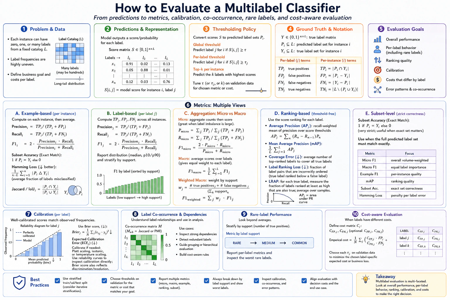
How would you evaluate a multilabel classifier? diagram
How to Explain It in an Interview
1. Define the prediction representation

For N observations and L labels, represent the model output as a score matrix S in [0,1]^(N x L). The element s_ij is the score for label j on observation i. The true labels can be represented as a binary matrix Y in {0,1}^(N x L), or as a true label set Y_i for each observation. The predicted label set is P_i.

2. Define the thresholding policy

A global threshold tau predicts label j when s_ij >= tau. If labels have different score distributions, prevalence, or error costs, use per-label thresholds tau_j and predict label j when s_ij >= tau_j. A top-k rule is another valid policy when the application explicitly needs a fixed number of highest-scoring labels. Tune tau, tau_j, or k on validation data for the chosen metric or cost. Do not choose the operating point on the final test set.

3. Measure example-based quality

Example-based metrics evaluate one observation at a time and then average across observations. For observation i, precision measures the fraction of predicted labels that are correct, recall measures the fraction of true labels that were recovered, and example F1 balances those two quantities. Jaccard or IoU is |P_i intersection Y_i| / |P_i union Y_i|. Hamming loss measures the average fraction of individual label decisions that are wrong. These metrics answer, 'How good is the predicted set for a typical observation?'

4. Measure label-based quality

Treat each label j as a one-versus-rest binary problem. Compute TP_j, FP_j, FN_j, precision_j, recall_j, and F1_j across all observations. This view is essential when frequencies are highly uneven because a strong aggregate result can hide labels with poor recall or precision. I would inspect the distribution of per-label metrics and stratify labels by support.

5. Compare micro and macro aggregation

Micro metrics aggregate TP, FP, and FN across labels before computing the score. For example, micro precision is sum_j TP_j / sum_j(TP_j + FP_j), and micro recall is sum_j TP_j / sum_j(TP_j + FN_j). Frequent labels therefore have more influence.

Macro F1 computes F1_j for each label and then averages equally: Macro-F1 = (1/L) sum_j F1_j. It gives rare labels the same weight as frequent labels. With a long-tailed label distribution, I would normally report both micro and macro results. A support-weighted F1 can be an additional summary, but it should not replace the unweighted macro view when rare labels matter.

6. Evaluate ranking quality before thresholding

Ranking metrics use the ordering of scores and do not require one final binary threshold. For label j, Average Precision is the recall-weighted mean of precision over thresholds: AP_j = sum_n (R_n - R_(n-1)) P_n. Mean Average Precision averages AP across labels.

LRAP is an example-aware ranking metric: for each true label, it checks how many labels ranked at least as high are also true, then averages across observations. Coverage error measures how far down the ranked list we must go to cover all true labels. Label ranking loss measures the fraction of true-versus-false label pairs that are ordered incorrectly. These metrics are useful when downstream systems consume ranked scores.

7. Report subset accuracy when exact-set correctness matters

Subset accuracy, or exact match, gives an observation a score of 1 only when P_i = Y_i; otherwise it gives 0. This is intentionally strict because one missing or extra label makes the whole observation incorrect. Use it when the full predicted label set must match exactly, and report it alongside less strict metrics rather than using it alone.

8. Inspect calibration per label

If scores are intended to behave like probabilities, inspect calibration separately for important labels. A reliability diagram compares mean predicted probability with observed frequency. A per-label Brier score is Brier_j = (1/N) sum_i (s_ij - y_ij)^2, where lower is better. Expected Calibration Error can also summarize reliability-bin deviations. Reliability diagrams show calibration directly; Brier score also reflects discrimination or resolution, so it should not be interpreted as a pure calibration measure by itself.

9. Inspect label co-occurrence and dependencies

Build a label co-occurrence matrix, for example using Jaccard similarity or pointwise mutual information. Use it to find labels that frequently appear together, redundant labels, or systematic paired errors. Then inspect whether the model often predicts one label in a common pair while missing the other. Co-occurrence is diagnostic evidence about label structure; it does not by itself prove causality.

10. Inspect rare-label errors explicitly

Break labels down by support and compare rare, medium, and common labels. Report per-label precision, recall, and F1, and inspect the worst rare labels instead of relying only on global averages. Macro metrics help because each label receives equal weight, while micro metrics can be dominated by frequent labels. For labels with very few positives, I would also report support because their metric estimates can be unstable.

11. Evaluate label-specific costs

If labels have different error costs, define C_FP,j for a false positive and C_FN,j for a false negative. One empirical cost summary is (1/N) sum_j(C_FP,j * FP_j + C_FN,j * FN_j). Choose each threshold tau_j on validation data to minimize the relevant label-specific expected cost or business loss. A costly-to-miss label may intentionally use a lower threshold to gain recall at the expense of more false positives.

12. Make the final decision from multiple views

I would not declare a winner from one metric. I would report micro and macro scores, per-label and example-based quality, ranking metrics when scores are consumed as rankings, subset accuracy when exact sets matter, calibration diagnostics when probabilities matter, co-occurrence and rare-label error slices, and the cost-aware operating thresholds. After all thresholds and policies are fixed on validation data, I would evaluate that frozen policy once on the held-out test set.

Technical Approach
  1. Represent model outputs as an N x L score matrix and ground truth as an N x L binary matrix or equivalent per-observation label sets.
  2. Define the prediction policy: global threshold, per-label thresholds, or top-k when the decision explicitly requires a fixed-size ranked set.
  3. Tune thresholds or k only on validation data using the target metric or label-specific cost.
  4. Compute example-based precision, recall, F1, Jaccard, and Hamming loss.
  5. Compute per-label TP, FP, FN, precision, recall, and F1.
  6. Report micro metrics for overall decision volume and macro metrics to give every label equal influence.
  7. Evaluate ranking quality with Average Precision or mAP, LRAP, coverage error, and label ranking loss when ranked scores matter.
  8. Report subset accuracy when the complete predicted label set must match exactly.
  9. Inspect per-label reliability diagrams, Brier score, and optionally ECE when calibrated probabilities matter.
  10. Analyze label co-occurrence using a suitable association matrix such as Jaccard or PMI and inspect paired error patterns.
  11. Stratify labels by support into rare, medium, and common groups and inspect the worst rare labels individually.
  12. Compute label-specific false-positive and false-negative costs and choose each tau_j on validation data to minimize the chosen cost or business loss.
  13. Freeze the full evaluation and thresholding policy and evaluate it once on the held-out test set.
Practical Insights

The main tradeoff is not computational complexity but evaluation complexity. With N observations and L labels, many calculations scale roughly with the N x L prediction matrix, and ranking metrics may need additional ordering work. Micro scores are stable for overall volume but can hide rare labels. Macro scores reveal rare-label problems but can be noisy when support is tiny. Exact match is easy to understand but very strict. Per-label thresholds, calibration checks, dependency analysis, and cost-aware evaluation require more validation work, but they better match real decisions when labels have uneven frequencies and different consequences.

Why Interviewers Ask This

This question tests whether the candidate understands that multilabel evaluation cannot be summarized safely by one accuracy number. The interviewer wants to see whether the candidate can define score and prediction representations, distinguish per-instance from per-label evaluation, explain micro versus macro behavior under severe label imbalance, evaluate ranking and exact-set correctness, inspect calibration and label dependencies, diagnose rare-label failures, and align threshold selection with label-specific false-positive and false-negative costs.

Common interview mistakes

Common mistakes are reporting only micro F1 and hiding rare-label failures; treating subset accuracy as the only useful metric; tuning thresholds on the test set; assuming one global threshold is appropriate even when labels have different costs; confusing Average Precision with simple geometric area under a precision-recall curve; treating example F1 as an exact-match metric; ignoring calibration when scores are used as probabilities; assuming label co-occurrence proves causality; and reporting aggregate scores without showing per-label support and the worst rare-label errors.

Interview tip

Use a clear order: scores and thresholds first, then example-based and per-label metrics, then micro versus macro, ranking, and exact match. Finish with calibration, co-occurrence, rare labels, and label-specific costs. State explicitly that no single metric is sufficient.
Interviewer may ask next
What would you do if a rare label has very few positive examples and its F1 score changes a lot between validation samples?

I would report that label's support together with precision, recall, and F1 instead of presenting F1 alone. I would compare it with other low-support labels and inspect its false positives and false negatives directly. I would also avoid interpreting a small difference in F1 as meaningful when the denominator is tiny. Threshold selection would still use validation data, but I would communicate the uncertainty and keep the per-label result visible rather than hiding it inside micro averages.

How would your evaluation change if false negatives for some labels became much more expensive than false positives?

I would keep the same broad metric suite but change the operating-point decision. For each affected label j, I would explicitly use its false-negative cost C_FN,j and false-positive cost C_FP,j and choose tau_j on validation data to minimize the relevant expected cost or business loss. That may intentionally lower the threshold and trade precision for higher recall. I would still report the other metrics so the cost-optimized policy does not hide ranking, calibration, rare-label, or exact-set failures.

12. What is hypothesis testing, and how does it support a data science decision?Statistics And ProbabilityEasy

Question Details

Define the null and alternative hypotheses, test statistic, significance level, p-value, Type I error, and Type II error. Explain the full decision process, including checking assumptions, selecting an appropriate test, interpreting statistical and practical significance, and communicating uncertainty without claiming that a test proves a hypothesis true.

Short Interview Answer (30-60 seconds)

Hypothesis testing uses sample data to measure evidence against a null hypothesis. I define H₀ and H₁, check assumptions, choose a suitable test, set α, compute a test statistic and p-value, and reject or fail to reject H₀. I also consider effect size, practical significance, and uncertainty.

Detailed Explanation

Hypothesis testing is a structured way to make a decision from sample data while recognizing uncertainty. The null hypothesis, H₀, is the default claim, such as no effect or no difference. The alternative hypothesis, H₁, is the competing claim. I first define the question, then check assumptions and choose an appropriate test. I set a significance level α, calculate a test statistic and p-value, and make a reject-or-fail-to-reject decision. I then consider effect size and practical significance. The test provides evidence; it does not prove either hypothesis true.

Useful Questions to Ask the Interviewer
  1. What decision or effect are we trying to evaluate?
  2. Are the observations independent, paired, clustered, or otherwise dependent?
  3. Which assumptions about the data and sampling process are justified?
  4. Should the alternative hypothesis be one-sided or two-sided?
  5. What size of effect would be large enough to matter in practice?
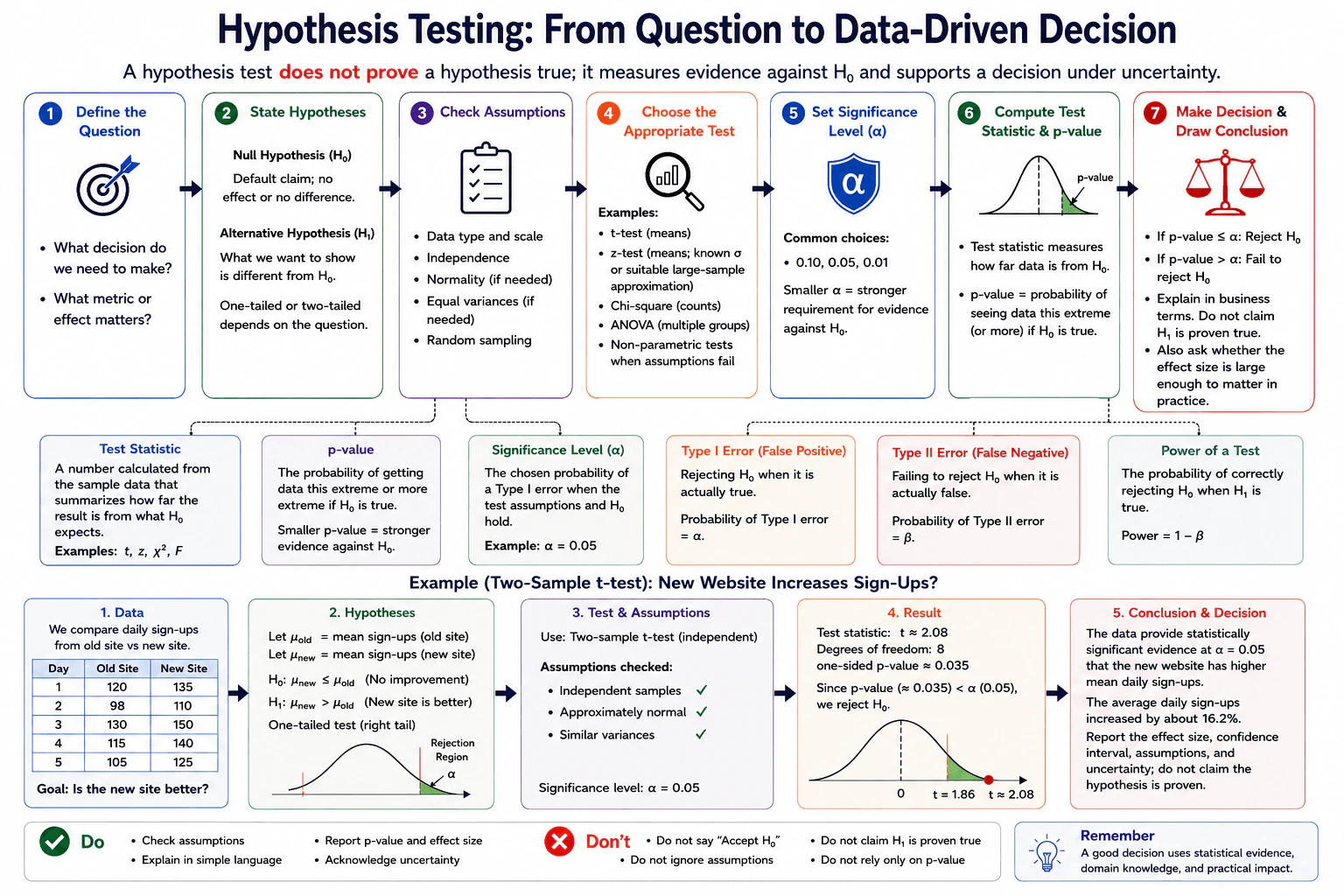
What is hypothesis testing, and how does it support a data science decision? diagram
How to Explain It in an Interview

Start with the decision. In the diagram example, the question is whether a new website has higher mean daily sign-ups than an old website. The observed daily sign-ups are 120, 98, 130, 115, and 105 for the old site, and 135, 110, 150, 140, and 125 for the new site.

Next, state the hypotheses. The null hypothesis H₀ is the default claim. In this example, H₀: μ_new ≤ μ_old, meaning the new site does not have a higher mean number of daily sign-ups. The alternative hypothesis is H₁: μ_new > μ_old. Because the question asks whether the new site is better in one specified direction, the example uses a one-sided test.

Then check assumptions before choosing a test. The diagram treats the two samples as independent, approximately normal, and similar in variance. More generally, I would check the observation structure, variable type, dependence, distribution assumptions, and sampling process. I would not automatically assume independence, normality, equal variance, or large-sample validity. The selected test must match the data and assumptions. Examples include a t-test for means, a z-test when its conditions are justified, a chi-square test for counts, ANOVA for several groups, or an appropriate non-parametric method when parametric assumptions are not reasonable.

Choose the significance level α before using the final test result. In the example, α = 0.05. Under the stated testing assumptions, α controls the probability of a Type I error: rejecting H₀ when H₀ is actually true. A Type II error means failing to reject H₀ when the specified alternative is actually true; its probability is β. Statistical power is 1 − β, the probability of rejecting H₀ when that specified alternative is true.

The test statistic is a number calculated from the sample that measures how far the observed result is from what H₀ would lead us to expect, using the scale defined by the chosen test. In the diagram's equal-variance independent two-sample t-test, the observed statistic is t ≈ 2.08 with 8 degrees of freedom.

The p-value is calculated from the test statistic and its reference distribution under H₀. It is the probability, assuming H₀ and the test assumptions are true, of observing a result at least as extreme as the one obtained in the direction specified by the test. It is not the probability that H₀ is true. The diagram's one-sided p-value is approximately 0.035.

The decision rule is: if the p-value is less than or equal to α, reject H₀; otherwise, fail to reject H₀. Here, approximately 0.035 < 0.05, so we reject H₀. The correct interpretation is that the data provide statistically significant evidence at α = 0.05 that the new website has higher mean daily sign-ups. We should not say that H₁ has been proven true. Likewise, failing to reject H₀ would not mean that H₀ had been proven or accepted as true.

Statistical significance is not the whole business decision. In the example, the old-site sample mean is 113.6 sign-ups per day and the new-site sample mean is 132.0. The observed increase is 18.4 sign-ups per day, or about 16.2% relative to the old-site mean. This effect size helps judge practical significance. A confidence interval, when reported, gives additional information about the range of effect sizes compatible with the data and helps communicate uncertainty.

Finally, communicate the result with context. Report the p-value, effect size, confidence interval when available, important assumptions, and limitations. Explain both statistical significance and whether the effect is large enough to matter in practice. A good data science decision combines statistical evidence, practical impact, domain knowledge, and uncertainty.

Technical Approach
  1. Define the decision and the effect being tested.
  2. State H₀ and H₁ clearly, including whether the alternative is one-sided or two-sided.
  3. Identify the observation structure and check assumptions such as independence, distributional conditions, and variance requirements.
  4. Choose a statistical test that matches the variable type, design, estimand, and justified assumptions.
  5. Choose the significance level α before using the final test result.
  6. Compute the test statistic and identify its reference distribution under H₀.
  7. Compute the p-value.
  8. If p-value ≤ α, reject H₀; otherwise, fail to reject H₀.
  9. Evaluate effect size and practical significance instead of relying only on the p-value.
  10. Report uncertainty, assumptions, limitations, and the decision without claiming that the test proves a hypothesis true.
Practical Insights

The numerical calculation for a basic hypothesis test is usually inexpensive. The harder work is deciding whether the test matches the data and whether its assumptions are reasonable. A smaller α lowers the tolerated Type I error probability but usually makes rejection harder and can increase Type II error unless other factors, such as sample size or effect size, change. More data can improve statistical power, but collecting data can cost time and money. A very small effect can also become statistically significant with enough data, so practical significance must be evaluated separately.

Why Interviewers Ask This

Interviewers want to see whether I can move correctly from sample evidence to a statistical decision. They are checking whether I understand H₀ and H₁, assumptions, test selection, test statistics, significance levels, p-values, Type I and Type II errors, statistical power, and the difference between statistical significance and practical significance. They also want to see whether I communicate uncertainty without claiming that a hypothesis test proves H₀ or H₁.

Common interview mistakes

Common mistakes include treating the p-value as the probability that H₀ is true, saying a significant result proves H₁, saying a non-significant result proves H₀, choosing α after seeing the result, ignoring whether observations are independent or paired, selecting a test without checking its assumptions, confusing statistical significance with practical importance, reporting only a p-value without effect size or uncertainty, and ignoring Type II error and statistical power.

Interview tip

Present hypothesis testing as one clear flow: question → H₀ and H₁ → assumptions → appropriate test → α → test statistic and p-value → reject or fail to reject H₀ → practical significance and uncertainty. Explicitly say that a hypothesis test provides evidence and does not prove a hypothesis true.

Interviewer may ask next
What would you do if the assumptions of the two-sample t-test in this example were not reasonable?

I would first identify which assumption fails. If the observations are paired, I would use a paired analysis instead of an independent-samples test. If equal variance is not reasonable, I would consider Welch's t-test rather than the equal-variance t-test. If the distributional assumptions are doubtful and the sample is too small for a reliable approximation, I would consider an appropriate non-parametric or resampling method. The replacement method still needs to match the same question, estimand, and observation structure.

What if the p-value were statistically significant but the observed effect were too small to matter in practice?

I would separate statistical significance from practical significance. I could report that the data provide statistically significant evidence against H₀ while also explaining that the estimated effect may be too small to justify action. I would report the effect size and its confidence interval and compare that effect with the size that matters for the decision. A small p-value does not tell us whether an effect is useful, valuable, or large enough to matter.

13. How would you explain a 95% confidence interval to a nontechnical stakeholder?Statistics And ProbabilityEasy

Question Details

Assume the interval was produced by a valid frequentist procedure for a population mean from a random sample. Explain what the 95% level does and does not mean, what repeated sampling has to do with coverage, and how sample size, variability, and model assumptions affect interval width and interpretation.

Short Interview Answer (30-60 seconds)

I would say a 95% confidence interval comes from a method that captures the true population mean in about 95% of repeated random samples. It does not mean there is a 95% chance the true mean is inside this one interval. Larger samples usually narrow the interval, while more variability widens it.

Detailed Explanation

A 95% confidence interval gives a range around an estimate of an unknown population mean. The population mean, written μ, is a fixed but unknown parameter. The sample mean, x̄, is an estimator used to learn about μ, and the value calculated from one sample is the estimate. The key point is that 95% describes the long-run performance of the interval-building procedure. If we repeatedly took random samples and built intervals in the same valid way, about 95% of those intervals would contain μ.

Useful Questions to Ask the Interviewer
  1. Should I focus on the frequentist interpretation of coverage rather than a Bayesian probability interpretation?
  2. May I assume the observations come from a random sample with the independence conditions needed by the procedure?
  3. Would you like a small numerical example to make the explanation more concrete?
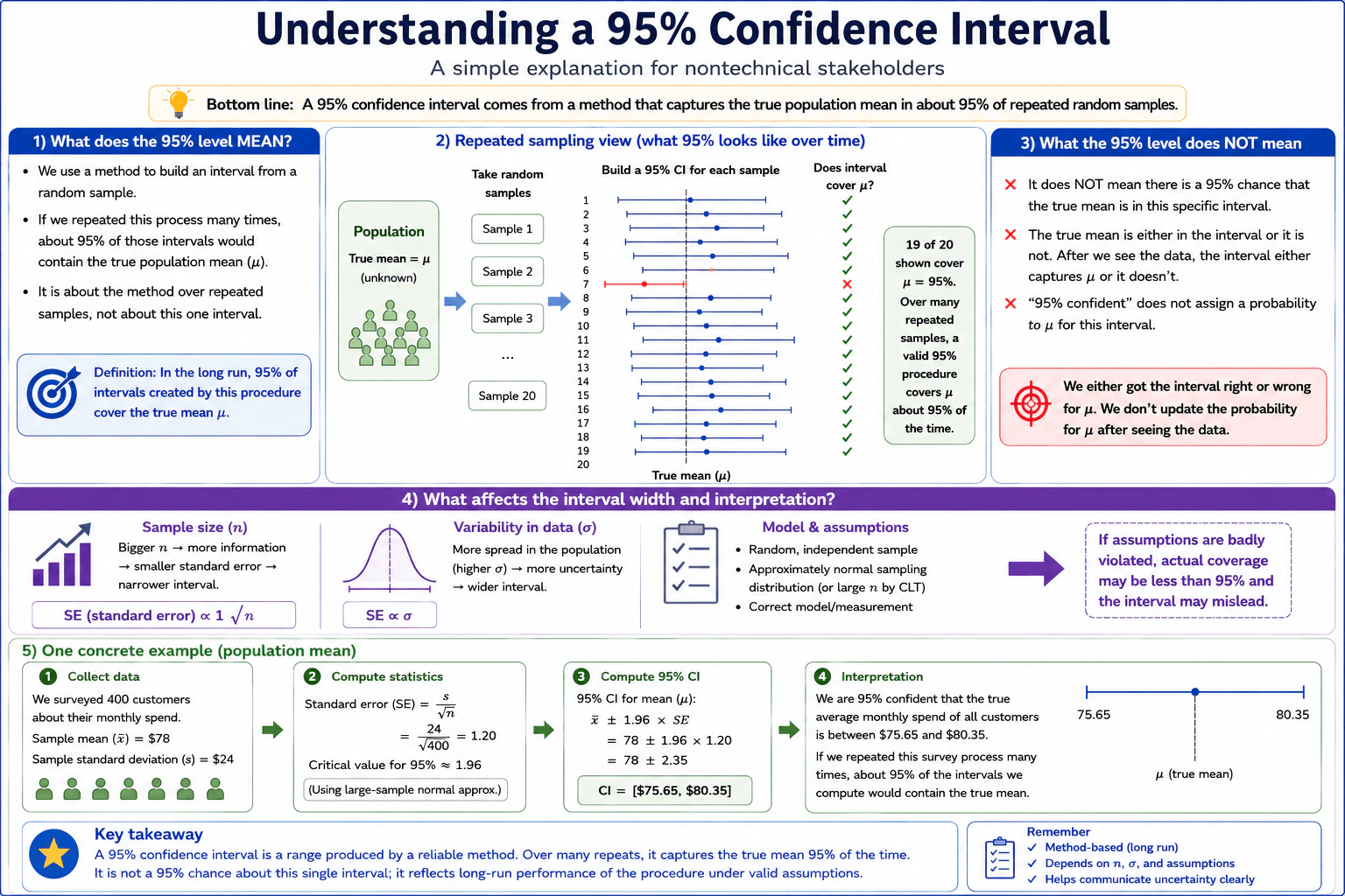
How would you explain a 95% confidence interval to a nontechnical stakeholder? diagram
How to Explain It in an Interview

Start with the quantity we want to estimate. The population mean μ is the true average for the target population. It is fixed, but we do not know its value. From a random sample, we calculate the sample mean x̄. The statistic x̄ is the estimator, and the value obtained from the observed sample is the estimate.

A confidence interval adds information about sampling uncertainty around that estimate. The key frequentist idea is repeated sampling. Imagine repeatedly drawing random samples from the same population and using the same valid procedure to create a 95% confidence interval each time. In the long run, about 95% of those intervals would contain the fixed true mean μ, while about 5% would miss it. The approved diagram illustrates this with 20 intervals: 19 cover μ and one misses it.

For the single interval we actually observed, I would avoid saying, "There is a 95% chance that μ is inside this interval." In the frequentist framework used here, μ is fixed rather than random. After the sample has been observed and the interval calculated, that particular interval either contains μ or it does not. The 95% describes the long-run coverage of the procedure, not a probability assigned to μ after seeing the data.

The interval width reflects uncertainty. In the large-sample example shown in the diagram, the interval has the form x̄ ± 1.96 × SE. Here x̄ is the sample mean and SE is the standard error of the sample mean. For an independent random sample, the standard error is estimated as s/√n, where s is the sample standard deviation and n is the sample size. A larger n usually makes the standard error smaller, roughly in proportion to 1/√n, so the interval becomes narrower. Greater variability makes the standard error larger and the interval wider.

The diagram's example uses 400 customers and monthly spending. The sample mean is $78 and the sample standard deviation is $24. The estimated standard error is 24/√400 = 1.20. Using the stated large-sample normal approximation, the 95% interval is 78 ± 1.96 × 1.20 = 78 ± 2.35, giving approximately [$75.65, $80.35]. A stakeholder-friendly statement is: "We are 95% confident that the true average monthly spending of the customer population is between $75.65 and $80.35." The important technical meaning behind that wording is the long-run 95% coverage of the procedure, not a 95% probability assigned to μ for this completed interval.

Finally, the interpretation depends on the assumptions that justify the procedure. The sample should be random, and observations should satisfy the independence conditions required by the method. The sampling distribution of the mean must also be adequately handled by the chosen procedure; with a sufficiently large sample, a normal approximation is often reasonable under standard conditions. The measurements and model must represent the intended population quantity correctly. If important assumptions are violated, the actual coverage may differ from 95%, and the interval can give a misleading impression of precision.

Technical Approach
  1. Identify the estimand: the fixed but unknown population mean μ.
  2. Use the sample mean x̄ as the estimator and calculate its observed estimate.
  3. Quantify sampling uncertainty with the standard error; for an appropriate independent random sample, estimate SE as s/√n.
  4. Build the 95% confidence interval using a procedure valid for the data and assumptions; in the diagram's large-sample example, use x̄ ± 1.96 × SE.
  5. Explain 95% as long-run coverage under repeated sampling, not as a 95% probability that μ lies in the completed interval.
  6. Explain that larger samples generally narrow the interval, greater variability widens it, and violated assumptions can make the stated coverage unreliable.
Practical Insights

The calculation itself is inexpensive. The important tradeoff is statistical precision. More observations usually make the interval narrower because the standard error decreases roughly as 1/√n. This means doubling the sample size does not cut the uncertainty in half. More variable data produce wider intervals. A narrow interval is not automatically trustworthy: poor sampling, dependence that is ignored, measurement problems, or invalid model assumptions can produce an interval that looks precise but does not have the intended 95% coverage.

Why Interviewers Ask This

Interviewers want to see whether the candidate can explain frequentist uncertainty accurately without using the common but incorrect interpretation that a completed interval has a 95% probability of containing the fixed population mean. They also test understanding of repeated-sampling coverage, the difference between a population parameter and a sample estimate, the factors that control interval width, and the importance of assumptions such as random sampling, appropriate independence, and a valid sampling-distribution approximation.

Common interview mistakes

The biggest mistake is saying that there is a 95% probability that the fixed population mean lies inside the particular interval already observed. Another mistake is saying that 95% of individual data values lie inside the confidence interval; this interval is about uncertainty in the population mean, not the spread of individual observations. Candidates may also forget that larger samples generally narrow the interval, greater variability widens it, and invalid sampling, dependence, measurement, or model assumptions can cause actual coverage to differ from 95%.

Interview tip

Lead with the repeated-sampling interpretation in one sentence, immediately state what 95% does not mean, and then explain sample size, variability, and assumptions. Use the simple numerical example if the stakeholder needs a concrete explanation.

Interviewer may ask next
What happens to the interpretation if the observations are not independent or the assumptions behind the interval are badly violated?

The nominal 95% level may no longer describe the procedure's actual coverage. For example, treating dependent observations as independent can underestimate the standard error and produce intervals that are too narrow. We should use a procedure that reflects the real sampling or dependence structure. If the assumptions supporting the method are materially violated, we should not claim that the interval reliably has 95% long-run coverage.

If we increase the sample size, what happens to the confidence interval, and is a narrower interval always better?

With the same underlying variability and an appropriate independent-sample procedure, increasing n reduces the standard error approximately as 1/√n, so the confidence interval usually becomes narrower. That means greater precision. However, a narrower interval is useful only when the sampling process, measurements, and statistical method are valid. A large biased or improperly modeled sample can produce a narrow interval around a misleading estimate, so precision does not replace sound assumptions.

14. What does a p-value mean?Statistics And ProbabilityEasy

Question Details

For a pre-specified null hypothesis and test statistic, define the p-value using the sampling distribution under the null. Explain what it does not say about the probability that either hypothesis is true, how it relates to a significance threshold, and why practical importance and confidence intervals still matter.

Short Interview Answer (30-60 seconds)

A p-value is the probability, assuming the null hypothesis is true, of getting a test statistic at least as extreme as the one observed. It does not tell us the probability that either hypothesis is true. We compare it with a chosen significance level and also consider effect size and confidence intervals.

Detailed Explanation

A p-value starts with a pre-specified null hypothesis, H0, and a chosen test statistic. We ask what values that statistic would have across repeated samples if H0 were true. This is its sampling distribution under H0. The p-value is the probability, within that distribution, of observing the actual test statistic or one at least as extreme in the direction or directions defined by the test. A small p-value means the observation is relatively unusual under H0. It does not tell us that H0 is probably false, and it does not measure how important an effect is.

Useful Questions to Ask the Interviewer
  1. Is the test one-sided or two-sided?
  2. What significance level, alpha, was chosen before looking at the result?
  3. What effect size and confidence interval should we consider together with the p-value?
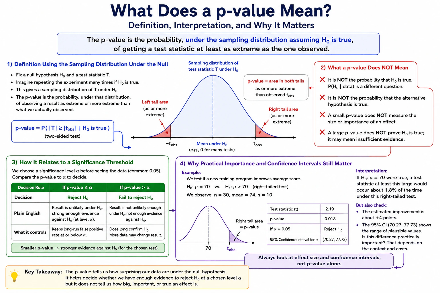
What does a p-value mean? diagram
How to Explain It in an Interview

Start with H0 and the test statistic. The test statistic summarizes the observed data in a way chosen for the hypothesis test. Under H0, that statistic has a reference, or sampling, distribution.

For a two-sided test, a common form is p-value = P(|T| >= |t_obs| | H0), where T is the test statistic under H0 and t_obs is the value calculated from the observed data. The p-value is the probability in the two relevant tails of obtaining a statistic at least as extreme as the observed one. For a one-sided test, only the tail specified by the alternative hypothesis is used.

The important conditioning is 'assuming H0 is true.' The p-value is not P(H0 | data). It is also not the probability that the alternative hypothesis is true. Frequentist hypothesis testing evaluates how compatible the observed statistic is with the null model; it does not directly assign probabilities to the hypotheses.

We normally choose a significance level, alpha, before examining the result. If p-value <= alpha, we reject H0 at that significance level. If p-value > alpha, we fail to reject H0. 'Fail to reject' does not mean that H0 has been proved true. It means the data did not provide sufficiently strong evidence against H0 for the chosen test and threshold.

For the example in the diagram, suppose a training program is tested with H0: mu = 70 and H1: mu > 70. The observed sample has n = 30, mean = 74, and s = 10. The diagram gives t approximately 2.19 and a right-tailed p-value of approximately 0.018. If H0: mu = 70 were true, a test statistic at least this large would occur about 1.8% of the time under this right-tailed test. With alpha = 0.05, 0.018 < 0.05, so we reject H0.

That decision still does not tell us whether the improvement is practically important. The estimated improvement over the null value is about 4 points. The shown 95% confidence interval for the population mean is approximately (70.27, 77.73). It gives a range of values that are reasonably compatible with the data under the confidence-interval procedure and its assumptions. Whether an improvement of this size matters depends on the context and costs. This is why a good statistical interpretation reports the p-value together with the effect size and confidence interval rather than using the p-value alone.

Technical Approach
  1. State the null hypothesis H0 and alternative hypothesis H1 before interpreting the result.
  2. Identify the test statistic and whether the test is one-sided or two-sided.
  3. Use the sampling distribution of that statistic under H0.
  4. Define the p-value as the probability, assuming H0 is true, of a statistic at least as extreme as the observed one in the direction or directions specified by the test.
  5. Compare the p-value with the pre-selected significance level alpha.
  6. If p-value <= alpha, reject H0; otherwise, fail to reject H0.
  7. Do not convert the p-value into a probability that either hypothesis is true.
  8. Report and interpret the effect size and confidence interval so statistical significance is not confused with practical importance.
Practical Insights

The main tradeoff is interpretation, not computational cost. A very small p-value can occur for a tiny effect when the sample is large, so statistical significance may not mean practical importance. A meaningful effect can also have a non-significant p-value when the sample is small or uncertainty is large. The significance threshold controls the decision rule, but changing alpha changes how strong the evidence must be before rejecting H0. Confidence intervals add useful information because they show the estimate together with its uncertainty.

Why Interviewers Ask This

Interviewers want to know whether the candidate understands statistical inference rather than only memorizing the rule p-value <= 0.05. A strong answer defines the p-value using the null sampling distribution, avoids treating it as the probability that a hypothesis is true, explains the role of a pre-selected significance level, and separates statistical significance from practical importance.

Common interview mistakes

Common mistakes are saying that a p-value is the probability that H0 is true, saying that 1 minus the p-value is the probability that H1 is true, treating p-value > alpha as proof that H0 is true, interpreting a small p-value as a large or important effect, forgetting whether the test is one-sided or two-sided, choosing alpha after seeing the result, and reporting statistical significance without the effect size or confidence interval.

Interview tip

Start with the phrase 'assuming the null hypothesis is true.' Then define the tail probability, explain the comparison with alpha, and immediately state what the p-value does not mean. Finish by saying that effect size and confidence intervals are needed to judge practical importance.

Interviewer may ask next
How does the interpretation change if the test is two-sided instead of right-tailed?

The basic meaning does not change: the p-value is still calculated from the sampling distribution under H0. What changes is which outcomes count as at least as extreme. In the right-tailed test H1: mu > 70, only sufficiently large positive test statistics contribute to the p-value. In a two-sided test H1: mu != 70, extreme results in both directions count, so the p-value includes both relevant tails. Therefore, the test direction should be chosen from the hypothesis before looking at the result.

If the p-value is 0.018, why do we still need the effect size and confidence interval?

The p-value describes how unusual the observed test statistic would be under H0 for the chosen test. It does not tell us how large or useful the effect is. In the example, the estimated improvement over the null value is about 4 points, while the 95% confidence interval for the population mean is approximately (70.27, 77.73). The estimate and interval help describe the size and uncertainty of the result. Whether that improvement is practically important depends on the context and costs, not on 0.018 alone.

15. What is statistical power?Statistics And ProbabilityEasy

Question Details

For a test with a specified null, alternative effect size, significance level, and sample-size plan, define power and its relationship to Type II error. Explain how power changes with effect size, variance, sample size, allocation, and multiple testing, and why post hoc interpretation of a nonsignificant result requires care.

Short Interview Answer (30-60 seconds)

Statistical power is the probability of correctly rejecting H0 when a specified alternative is true. Power equals 1 − β, where β is the Type II error rate. Larger effects, larger samples, lower variance, and efficient allocation usually increase power. Stricter multiple-testing corrections usually reduce it, and nonsignificance does not prove no effect.

Detailed Explanation

Statistical power asks: if the alternative hypothesis is true at a specified effect size, how likely is the test to reject the null hypothesis? That probability is power. If β is the probability of failing to reject the null when that alternative is true, then power = 1 − β. Power depends on the planned test, effect size, significance level, sample size, variance, and allocation. A larger signal or more precise data usually raises power. Multiple-testing corrections usually lower it. A nonsignificant result therefore needs careful interpretation because low power can hide a meaningful effect.

Useful Questions to Ask the Interviewer
  1. What null hypothesis and alternative effect size should I use for the power calculation?
  2. What significance level, such as α = 0.05, is planned?
  3. Is the test one-sided or two-sided?
  4. What sample size and group allocation are planned?
  5. What variance or standard deviation should I assume for planning?
  6. Will we test one hypothesis or adjust for multiple tests?
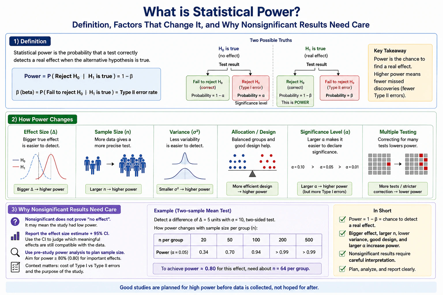
What is statistical power? diagram
How to Explain It in an Interview

Start with the two possible truths. Under H0, the null hypothesis is true. Under the specified H1, a real effect of the planned size exists.

If H1 is true and the test rejects H0, the test correctly detects the effect. The probability of that event over repeated samples is statistical power:

Power = P(reject H0 | H1 is true) = 1 − β.

Here, β is the Type II error probability:

β = P(fail to reject H0 | H1 is true).

A Type II error means missing a real effect of the specified size. Higher power therefore means a lower chance of missing that specified alternative.

For completeness, α is the Type I error probability under H0. With the rest of the design fixed, increasing α makes rejection easier and generally increases power, but it also allows more Type I errors. Decreasing α does the opposite unless another design factor, such as sample size, changes.

Effect size matters because a larger true difference is easier to distinguish from random variation. So, with the other inputs fixed, a larger effect size gives higher power.

Variance works in the opposite direction. Greater variability creates more noise relative to the signal. Lower variance usually gives more precise estimates and therefore higher power.

Sample size is one of the main design controls. More observations usually reduce sampling uncertainty, so a test can detect a specified difference more reliably. In the diagram's two-sample mean-test example, Δ = 5 units, σ = 10, the test is two-sided, and α = 0.05. Power is about 0.34 with n = 20 per group, 0.70 with n = 50, 0.94 with n = 100, and greater than 0.99 with n = 200 or 500. For this planned effect and test, about n = 64 per group gives power near 0.80.

Allocation also matters. For many two-group comparisons with similar group variances and observation costs, balanced group sizes are more efficient than very unequal group sizes for the same total sample size. The best allocation can change when group variances, costs, or other design constraints differ.

Multiple testing matters because testing many hypotheses creates more opportunities for false positives. A multiplicity correction can use stricter rejection thresholds or another adjusted procedure. Holding the rest of the design fixed, this generally reduces the power of an individual test because rejection becomes harder. The power calculation should use the same multiple-testing procedure planned for the final analysis.

Finally, a nonsignificant result does not prove that the effect is zero. A study can fail to reject H0 because the true effect is small, the sample is too small, the variance is high, or the test otherwise has limited power. After observing the data, reporting observed post hoc power usually adds little because it is largely determined by the observed effect and p-value. Instead, report the estimated effect and its confidence interval. The confidence interval helps show which effect sizes are still reasonably compatible with the data. Power is most useful before data collection, when planning a sample size for an effect that is scientifically or practically important.

Technical Approach
  1. Specify H0 and the alternative effect size that matters.
  2. Choose the significance level α and whether the test is one-sided or two-sided.
  3. Specify the variance or standard-deviation assumption required for the planned test.
  4. Specify the total sample size and allocation between groups.
  5. Compute or simulate β under the specified alternative, then calculate power = 1 − β.
  6. If power is too low, consider a larger sample, lower measurement variance, a more efficient allocation, or another scientifically justified design change.
  7. If multiple hypotheses are tested, calculate power using the actual multiplicity-adjusted procedure.
  8. After the study, interpret a nonsignificant result using the estimated effect and confidence interval instead of treating nonsignificance as proof of no effect.
Practical Insights

Higher power is useful, but it has tradeoffs. Increasing sample size requires more observations, time, or cost. Reducing variance may require better measurements or tighter experimental control. Balanced allocation is often efficient, although unequal allocation can be reasonable when group costs or variances differ. Increasing α raises power but also raises the Type I error rate. Multiple-testing corrections reduce false-positive risk across many tests, but stricter rejection rules usually make real effects harder to detect. Power is also specific to the assumed effect size and test design; it is not one permanent number that describes a study under every possible alternative.

Why Interviewers Ask This

Interviewers want to see whether you understand what a hypothesis test can and cannot detect. They also want you to connect power to Type II error, explain how effect size, variance, sample size, allocation, significance level, and multiple testing affect power, and avoid treating a nonsignificant result as proof that no effect exists.

Common interview mistakes

Common mistakes are saying that power is the probability that H1 is true, confusing β with power instead of using power = 1 − β, assuming a nonsignificant p-value proves there is no effect, calculating power without specifying an alternative effect size, ignoring variance or allocation, forgetting the tradeoff between α and Type I error, and ignoring the loss of power caused by stricter multiple-testing procedures. Another mistake is using observed post hoc power after a nonsignificant result as if it provides new evidence. Report the effect estimate and confidence interval instead, and keep statistical significance separate from practical importance.

Interview tip

Start with: 'Power is the probability of rejecting H0 when the specified alternative is true.' Then write power = 1 − β. Explain the main drivers: effect size, variance, sample size, allocation, α, and multiple testing. Finish by saying that a nonsignificant result is not proof of no effect and should be interpreted with the effect estimate and confidence interval.

Interviewer may ask next
If the planned sample size stays the same but the true effect is smaller than the effect used in the power calculation, what happens?

Power decreases. A smaller true effect is harder to distinguish from random variation, so the probability of rejecting H0 becomes lower when the other design inputs stay fixed. This is why power must always be tied to a specified alternative effect size. A study can have high power for a large effect but low power for a smaller one. In the diagram's example, Δ = 5 and σ = 10 are used for planning. If the true difference were smaller while n, σ, α, allocation, and the testing procedure stayed unchanged, power would be lower.

What happens to power if we add a multiple-testing correction while keeping the sample size unchanged?

Power generally decreases for an individual hypothesis because the corrected procedure makes rejection harder. For example, a correction may use a stricter per-test threshold than an unadjusted α = 0.05 test. This reduces false positives across the family of tests, but it also makes true effects harder to detect. To recover power, the study may need a larger sample, lower variance, a more efficient design, or a larger true effect. The correct power calculation should use the same multiple-testing procedure planned for the final analysis.

16. A disease affects 0.1% of people. A test has 98% sensitivity and a 1% false-positive rate. What is the probability that a person who tests positive has the disease?Statistics And ProbabilityEasy

Question Details

Use Bayes' rule with prevalence P(D)=0.001, sensitivity P(+|D)=0.98, and false-positive rate P(+|not D)=0.01. Calculate P(D|+) and explain why the base rate changes the interpretation of an apparently accurate test.

Short Interview Answer (30-60 seconds)

I would use Bayes' rule. The true-positive probability is 0.98 × 0.001 = 0.00098, while the false-positive probability is 0.01 × 0.999 = 0.00999. So P(D|+) = 0.00098 / 0.01097 ≈ 0.0893, or about 8.93%.

Detailed Explanation

The goal is to find the probability that a person has the disease after receiving a positive test. This is P(D|+), not the test's 98% sensitivity. The disease prevalence is P(D)=0.001, so P(not D)=0.999. A person with the disease tests positive with probability 0.98, while a person without the disease tests positive with probability 0.01. Bayes' rule combines these probabilities. The important idea is the base rate: because the disease is very rare, false positives from the much larger healthy group can greatly outnumber true positives.

Useful Questions to Ask the Interviewer
  1. Should I assume the stated prevalence, sensitivity, and false-positive rate all apply to the same population being tested?
  2. Should I report the final probability as a percentage rounded to two decimal places?
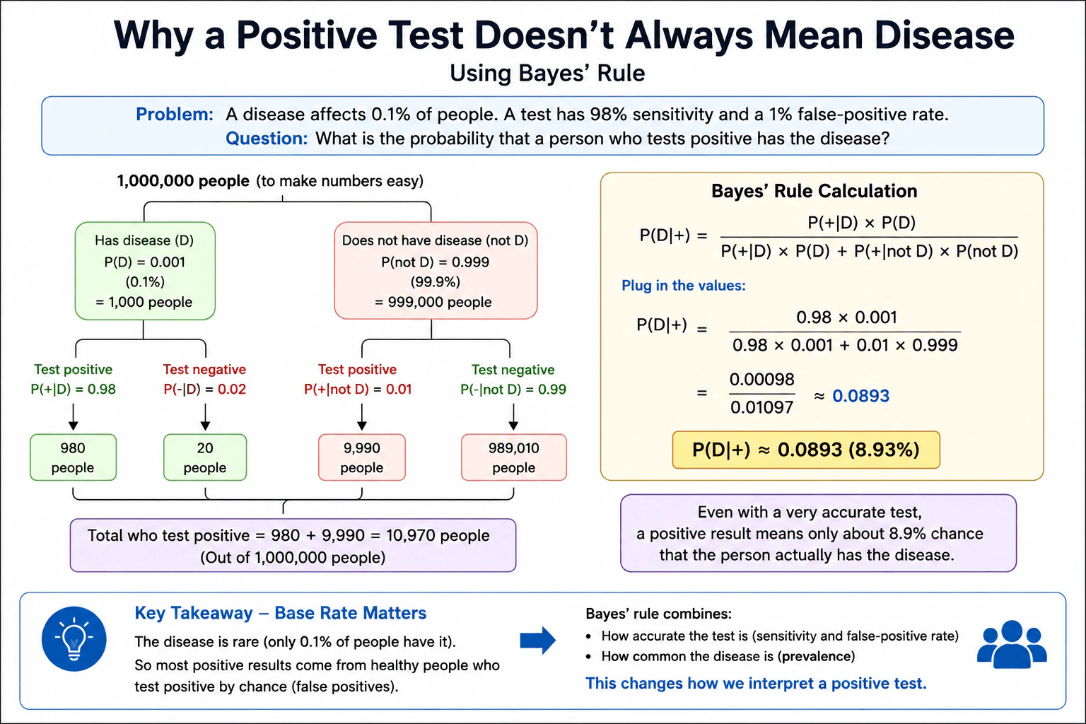
A disease affects 0.1% of people. A test has 98% sensitivity and a 1% false-positive rate. What is the probability that a person who tests positive has the disease? diagram
How to Explain It in an Interview

We want P(D|+), which means the probability that a person has the disease given that the test result is positive.

The supplied probabilities are:

  • P(D) = 0.001, the prevalence or base rate.
  • P(not D) = 1 - 0.001 = 0.999.
  • P(+|D) = 0.98, the sensitivity or true-positive rate.
  • P(+|not D) = 0.01, the false-positive rate.

Bayes' rule is: P(D|+) = [P(+|D) × P(D)] / [P(+|D) × P(D) + P(+|not D) × P(not D)].

Substitute the values: P(D|+) = (0.98 × 0.001) / [(0.98 × 0.001) + (0.01 × 0.999)].

The true-positive joint probability is: 0.98 × 0.001 = 0.00098.

The false-positive joint probability is: 0.01 × 0.999 = 0.00999.

Therefore, the probability of any positive result is: P(+) = 0.00098 + 0.00999 = 0.01097.

Now divide: P(D|+) = 0.00098 / 0.01097 ≈ 0.0893 = 8.93%.

The same reasoning can be shown with 1,000,000 people, matching the diagram. About 1,000 people have the disease. With 98% sensitivity, 980 of them test positive and 20 test negative. About 999,000 people do not have the disease. With a 1% false-positive rate, 9,990 of them test positive and 989,010 test negative. There are therefore 10,970 positive tests in total, but only 980 are true positives. So 980 / 10,970 ≈ 8.93%.

The key interpretation is that sensitivity is not P(D|+). Sensitivity answers, 'If someone has the disease, how often is the test positive?' The question asks the reverse conditional probability: 'If someone tests positive, how likely is it that they have the disease?' Because only 0.1% of people have the disease, the base rate is so low that false positives from the much larger healthy population dominate the positive results.

Technical Approach
  1. Identify the target probability as P(D|+).
  2. Compute P(not D)=1-P(D)=0.999.
  3. Compute the true-positive joint probability: P(+|D) × P(D)=0.98 × 0.001=0.00098.
  4. Compute the false-positive joint probability: P(+|not D) × P(not D)=0.01 × 0.999=0.00999.
  5. Add them to get P(+)=0.01097.
  6. Divide the true-positive joint probability by the total positive probability: 0.00098/0.01097≈0.0893.
  7. Convert to a percentage and round at the end: about 8.93%.
Practical Insights

This calculation uses only a few arithmetic operations, so the computational cost is constant and negligible. The important issue is statistical interpretation. The result depends strongly on the disease prevalence. Even with high sensitivity and a low false-positive rate, a rare disease can have a low probability of being present after a positive result because the healthy population is much larger.

Why Interviewers Ask This

This question tests whether a candidate can apply conditional probability and Bayes' rule correctly, distinguish sensitivity from the probability of disease after a positive result, and recognize the importance of the base rate. It also tests whether the candidate can explain why a seemingly accurate test may still produce mostly false-positive results when the condition is rare.

Common interview mistakes

A common mistake is answering 98%, but 98% is P(+|D), the sensitivity, not P(D|+), which is what the question asks. Another mistake is ignoring the 0.1% prevalence. It is also wrong to use the 1% false-positive rate by itself in the denominator; it must be weighted by P(not D)=0.999. Finally, avoid rounding intermediate values too early.

Interview tip

Start by stating that the question asks for P(D|+), while sensitivity gives P(+|D). Then write Bayes' rule, substitute the supplied probabilities, calculate 8.93%, and finish by explaining that the low base rate creates many more false positives than true positives.

Interviewer may ask next
What assumption is important when using the given prevalence, sensitivity, and false-positive rate in Bayes' rule?

We assume that the stated prevalence, sensitivity, and false-positive rate apply to the same population as the person being tested. In particular, the 0.1% prevalence must be an appropriate prior probability for that population. If the population has a different prevalence or the test behaves differently there, P(D|+) will change.

Why can a test with 98% sensitivity still give only about an 8.93% probability of disease after a positive result?

The disease is very rare. In the 1,000,000-person example, 980 diseased people test positive, but 9,990 healthy people also test positive. Therefore, only 980 of the 10,970 positive results are true positives. That ratio is about 8.93%. The large number of healthy people makes the base rate critical.

17. A fair six-sided die is rolled twice. What is the probability that the first roll is 1 and the second roll is not 6?Statistics And ProbabilityEasy

Question Details

Treat the two rolls as independent, enumerate the event on each roll, and give the exact probability as a fraction. State how the calculation would change if the second roll were conditionally dependent on the first.

Short Interview Answer (30-60 seconds)

The first roll must be 1, which has probability 1/6. The second roll can be 1, 2, 3, 4, or 5, so its probability is 5/6. Because the rolls are independent, I multiply them: (1/6) × (5/6) = 5/36.

Detailed Explanation

A fair six-sided die has six equally likely outcomes on each roll. We need the event where the first roll is exactly 1 and the second roll is anything except 6. For the first roll, the allowed set is {1}. For the second roll, the allowed set is {1, 2, 3, 4, 5}. Because the rolls are independent, the first result does not change the probabilities on the second roll. Therefore, we multiply 1/6 by 5/6. This gives the exact probability 5/36, which also matches five favorable ordered pairs out of 36 equally likely pairs.

Useful Questions to Ask the Interviewer
  1. Should I show both the multiplication method and the ordered-pair enumeration?
  2. If you want a dependent version too, should I express it using a general conditional probability or use a specific dependence rule?
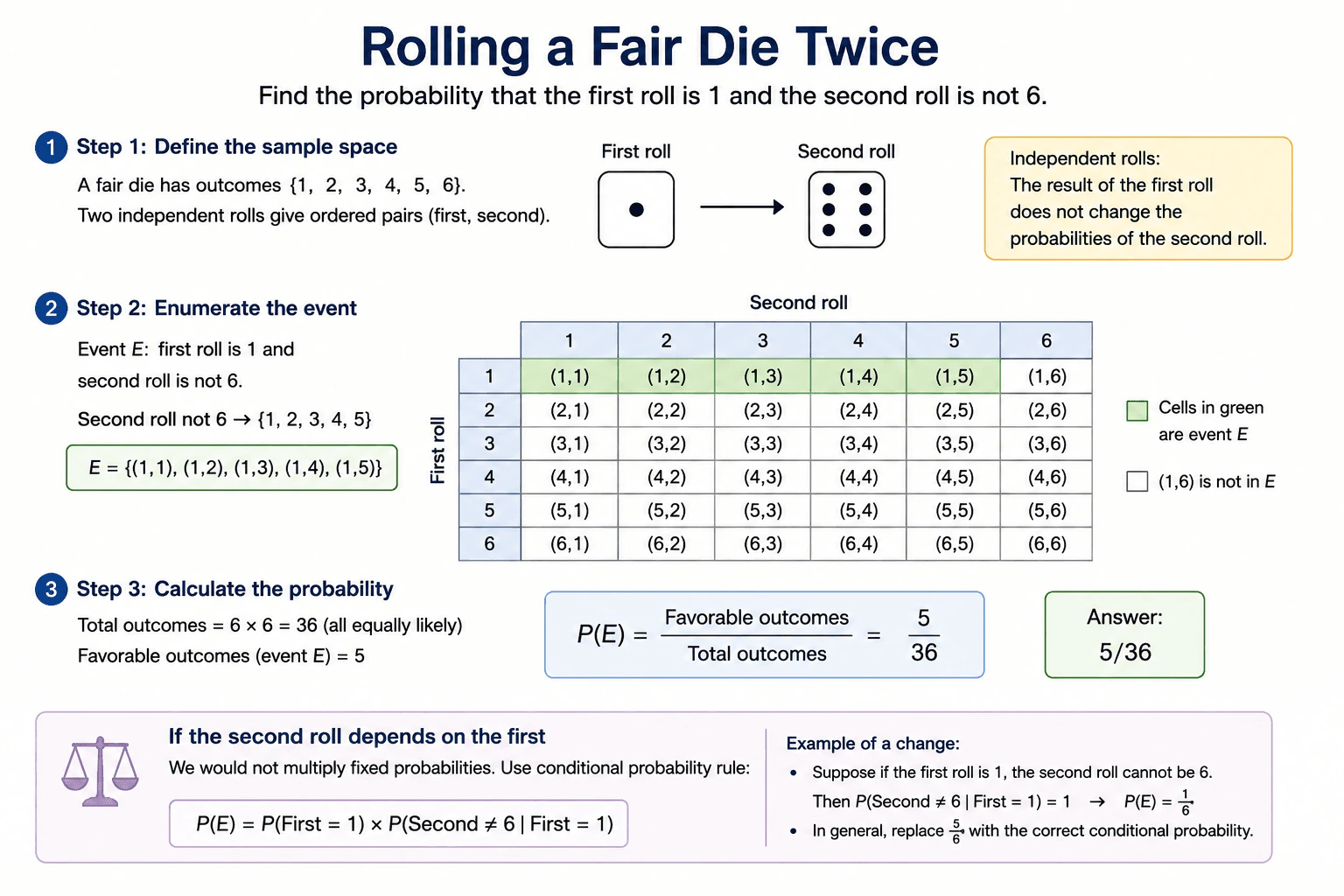
A fair six-sided die is rolled twice. What is the probability that the first roll is 1 and the second roll is not 6? diagram
How to Explain It in an Interview

Let A be the event that the first roll is 1. Since the die is fair, P(A) = 1/6.

Let B be the event that the second roll is not 6. The allowed outcomes are {1, 2, 3, 4, 5}, so P(B) = 5/6.

The two rolls are independent. Independence means the result of the first roll does not change the probability distribution of the second roll. Therefore,

P(A and B) = P(A) × P(B) = (1/6) × (5/6) = 5/36.

We can verify the same result by enumerating ordered pairs. There are 6 × 6 = 36 equally likely ordered outcomes. The event contains exactly five outcomes: {(1,1), (1,2), (1,3), (1,4), (1,5)}. The pair (1,6) is excluded because the second roll must not be 6. Thus the probability is 5/36.

If the second roll were conditionally dependent on the first, we would not automatically use 5/6 for the second event. Instead, we would use

P(A and B) = P(A) × P(B | A),

where P(B | A) means the probability that the second roll is not 6 given that the first roll was 1. For the example shown in the diagram, suppose the second roll cannot be 6 when the first roll is 1. Then P(B | A) = 1, so the event probability becomes (1/6) × 1 = 1/6.

Technical Approach
  1. Define the first-roll event: first roll = 1, so its probability is 1/6.
  2. Define the second-roll event: second roll is not 6, so the valid outcomes are {1, 2, 3, 4, 5} and its probability is 5/6.
  3. Because the rolls are independent, multiply the probabilities.
  4. Compute (1/6) × (5/6) = 5/36.
  5. Check the result by counting five favorable ordered pairs among 36 equally likely ordered pairs.
  6. If dependence is introduced, replace P(second roll is not 6) with P(second roll is not 6 | first roll = 1).
Practical Insights

There is almost no computational cost because the problem has only two rolls and six possible values per roll. Direct multiplication is the shortest method. Enumerating all 36 ordered pairs takes more work but provides a useful check. The important statistical issue is the independence assumption: using the fixed probability 5/6 for the second event is valid only when the first roll does not change the second-roll probabilities.

Why Interviewers Ask This

This question tests whether you can identify events, use independence correctly, count equally likely outcomes, and switch to conditional probability when dependence is introduced. It also checks whether you can explain a simple probability calculation clearly instead of applying a multiplication rule without stating its assumptions.

Common interview mistakes

Common mistakes are adding 1/6 and 5/6 instead of multiplying them, treating 'not 6' as only one outcome instead of five, including the excluded pair (1,6), using the wrong total instead of 36 ordered outcomes, or continuing to use P(A) × P(B) after dependence is introduced. In the dependent case, use P(A) × P(B | A).

Interview tip

State the independence assumption before multiplying. Then show the compact calculation, (1/6) × (5/6) = 5/36, and use the five favorable ordered pairs out of 36 as a quick verification. If dependence is introduced, switch immediately to conditional probability.

Interviewer may ask next
Why can we multiply 1/6 by 5/6 in the original problem?

Because the two rolls are independent. The first roll does not change the probabilities on the second roll. Therefore, P(first = 1 and second ≠ 6) = P(first = 1) × P(second ≠ 6) = (1/6) × (5/6) = 5/36.

How does the answer change if the second roll cannot be 6 whenever the first roll is 1?

Then the second roll is conditionally dependent on the first. We use P(first = 1) × P(second ≠ 6 | first = 1). Under this rule, P(second ≠ 6 | first = 1) = 1, so the probability becomes (1/6) × 1 = 1/6.

18. How would you derive a confidence interval for a coin's probability of heads?Statistics And ProbabilityMedium

Question Details

A coin is tossed n independent times and produces h heads. Define the estimand p, derive or justify a two-sided 95% interval using an appropriate binomial method, and compare the normal approximation with an exact or score-based alternative when n is small or h is near 0 or n.

Short Interview Answer (30-60 seconds)

I would model the head count as H ~ Binomial(n, p), estimate p with p̂ = h/n, and prefer a Wilson 95% interval. The Wald interval is simple but unreliable for small n or extreme counts; Clopper-Pearson is exact but conservative.

Detailed Explanation

The unknown quantity is p, the coin's true probability of heads. Each toss is one Bernoulli observation, and the question states that the n tosses are independent. Assuming the probability of heads stays constant across tosses, the total number of heads H follows Binomial(n, p). After observing h heads, the estimator is p̂ = H/n and its observed estimate is h/n. The goal is a two-sided 95% confidence interval for p. The main choice is between a simple normal approximation, a Wilson score interval, and an exact binomial interval.

Useful Questions to Ask the Interviewer
  1. Should I emphasize a practical default interval, such as Wilson, or derive several common alternatives?
  2. Do you want a conservative finite-sample coverage guarantee, or is a score-based interval with better practical behavior sufficient?
  3. Should I show how the methods behave when the observed number of heads is close to 0 or n?
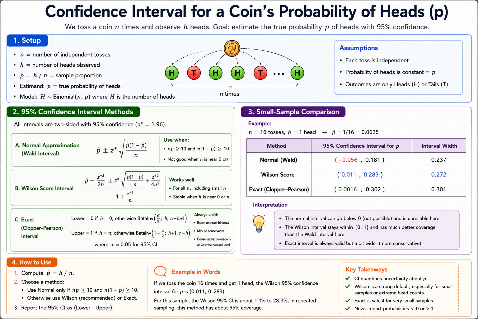
How would you derive a confidence interval for a coin's probability of heads? diagram
How to Explain It in an Interview

Start with the statistical model. Let p be the estimand: the fixed but unknown probability that one toss produces heads. Let H be the random number of heads in n independent tosses. Under a constant head probability, H ~ Binomial(n, p). The estimator is p̂ = H/n. Once we observe h heads, the numerical estimate is p̂ = h/n.

For a two-sided 95% interval, the simplest large-sample method is the normal or Wald interval:

p̂ ± z*√(p̂(1-p̂)/n),

where z* = 1.96 for 95% confidence. This comes from approximating the sampling distribution of p̂ by a normal distribution with standard error √(p(1-p)/n), then replacing the unknown p by p̂. A common practical check is that n p̂ and n(1-p̂) are both at least about 10. When this fails, especially when h is near 0 or n, the approximation can have poor coverage and can even produce endpoints below 0 or above 1.

A better score-based choice is the Wilson interval. With z = 1.96, it is

[p̂ + z²/(2n) ± z√(p̂(1-p̂)/n + z²/(4n²))] / [1 + z²/n].

The Wilson interval comes from inverting the binomial score test rather than centering a normal interval directly at p̂. It behaves much better for small samples and extreme observed proportions and stays inside the valid probability range [0, 1]. This makes Wilson a strong practical default.

An exact alternative is the two-sided Clopper-Pearson interval, obtained by inverting exact binomial tail probabilities. For α = 0.05, its limits can be written using beta-distribution quantiles. The lower limit is 0 when h = 0; otherwise it is BetaInv(α/2; h, n-h+1). The upper limit is 1 when h = n; otherwise it is BetaInv(1-α/2; h+1, n-h). This interval has coverage at least the nominal level, but it is usually conservative, so it can be wider than necessary.

For the diagram's example, n = 16 and h = 1, so p̂ = 1/16 = 0.0625. The raw Wald 95% interval is about (-0.056, 0.181), with width about 0.237. It includes an impossible negative probability and shows why the normal approximation is unreliable here. The Wilson interval is about (0.011, 0.283), with width about 0.272. The exact Clopper-Pearson interval is about (0.0016, 0.302), with width about 0.301. Wilson gives a useful compromise between coverage behavior and interval width, while the exact method is wider because it is conservative.

The confidence interpretation is frequentist. After observing this sample, I would report the Wilson 95% interval as about 1.1% to 28.3%. I would not say there is a 95% probability that the fixed p lies in this particular interval. Instead, if we repeatedly generated samples under the same model and rebuilt intervals using the same procedure, the Wilson method has coverage close to 95% in this setting. For Clopper-Pearson, the actual coverage is at least the nominal level and is often higher.

Technical Approach

1. Define p as the true probability of heads. 2. Model the observed head count as H ~ Binomial(n, p), assuming independent tosses and the same p for every toss. 3. Compute the observed proportion p̂ = h/n. 4. Check whether the normal approximation is reasonable using n p̂ and n(1-p̂). Values around 10 or larger support the approximation. 5. If the approximation is adequate, the Wald interval is p̂ ± 1.96√(p̂(1-p̂)/n), although Wilson is still a strong choice. 6. If n is small or h is near 0 or n, prefer the Wilson score interval. 7. If conservative finite-sample binomial coverage is important, use the exact Clopper-Pearson interval. 8. Do not report an impossible probability endpoint below 0 or above 1. If the raw Wald interval produces one, use a method such as Wilson or Clopper-Pearson that respects the parameter space. 9. Interpret 95% confidence as a repeated-sampling coverage property of the procedure.

Practical Insights

All three methods are inexpensive for a single coin experiment. The Wald interval needs only basic arithmetic and is the simplest, but simplicity comes with poor behavior for small samples or proportions near 0 or 1. Wilson needs a slightly longer formula but usually gives much better coverage behavior and stays within [0, 1]. Clopper-Pearson requires binomial-tail or beta-quantile calculations. It gives conservative coverage of at least the nominal level, but that safety often makes the interval wider. The important tradeoff is therefore statistical reliability versus simplicity and, for the exact method, interval width.

Why Interviewers Ask This

This question tests whether a candidate can distinguish the unknown parameter p from the estimator p̂, use the binomial model correctly, state the independence and constant-probability assumptions, construct uncertainty around a proportion, recognize when a normal approximation is unreliable, and choose between Wald, Wilson score, and exact binomial intervals. It also tests whether the candidate interprets a 95% confidence interval using repeated-sampling coverage rather than saying there is a 95% probability that the fixed parameter lies inside the observed interval.

Common interview mistakes

Common mistakes are confusing the unknown parameter p with the estimator p̂ = H/n or the observed estimate h/n; using the Wald interval automatically when n is small; ignoring that the Wald interval can extend below 0 or above 1; assuming normal-approximation validity without checking the observed success and failure counts; saying the exact Clopper-Pearson interval is always the narrowest or most accurate when it is usually conservative; forgetting the h = 0 and h = n boundary cases in the exact beta-quantile formulas; and interpreting a 95% frequentist confidence interval as giving a 95% probability that the fixed p lies inside the particular observed interval.

Interview tip

Define p, H, and p̂ first. Then give the Wald formula briefly, explain why it can fail near the boundaries, and recommend Wilson as the practical default with Clopper-Pearson as the conservative exact alternative. Finish with the correct repeated-sampling interpretation of 95% confidence.

Interviewer may ask next
What happens to these confidence-interval methods when the observed number of heads is at an extreme, such as h = 0 or h = n?

The Wald interval is especially unreliable at an extreme because p̂ is 0 or 1, making its plug-in standard error zero and producing a degenerate interval. Wilson still gives a nonzero interval and keeps the endpoints inside [0, 1]. The exact Clopper-Pearson method also handles the boundary correctly: its lower endpoint is defined as 0 when h = 0, and its upper endpoint is defined as 1 when h = n. This is why Wilson or an exact binomial interval is preferred near the boundaries.

For the n = 16, h = 1 example, why might you choose Wilson instead of the exact Clopper-Pearson interval?

Both avoid the poor Wald behavior. Wilson gives about (0.011, 0.283), while Clopper-Pearson gives about (0.0016, 0.302). The exact interval is wider because it is conservative and provides coverage at least as large as the nominal level. If I want a strong practical interval with good coverage behavior and less conservatism, I would choose Wilson. If conservative finite-sample coverage is the priority, I would choose Clopper-Pearson.

19. Customer lifetimes are independent exponential random variables. How would you estimate the rate parameter?Statistics And ProbabilityMedium

Question Details

Given observed positive lifetimes x1 through xn from an exponential distribution with density λ exp(-λx), derive the likelihood and the maximum-likelihood estimator of λ. State the assumptions, the corresponding estimator of mean lifetime, and what censoring would change.

Short Interview Answer (30-60 seconds)

Assuming the positive customer lifetimes are independent and exactly observed, I write the exponential likelihood and maximize it. This gives λ̂ = n/Σxi = 1/x̄. Since mean lifetime is 1/λ, its estimate is x̄. Right censoring changes the likelihood because censored observations contribute survival probabilities rather than density values.

Detailed Explanation

Let Xi be the lifetime of customer i, measured from acquisition, and assume X1,...,Xn are independent and identically distributed Exponential(λ) random variables with λ > 0. The observed lifetimes xi are positive and, initially, exactly observed with no censoring. The unknown parameter λ is the event rate per unit time. The estimand is this common population rate. We derive an estimator from the likelihood of the observed data. In the diagram example, the five lifetimes are 2.1, 0.7, 1.3, 3.0, and 0.4 time units.

Useful Questions to Ask the Interviewer
  1. Are all customer lifetimes fully observed, or are some customers still active and therefore right-censored?
  2. Can I assume the lifetimes are independent and follow one common exponential distribution with a constant rate λ?
  3. Are all lifetimes measured from the same time origin and in the same time units?
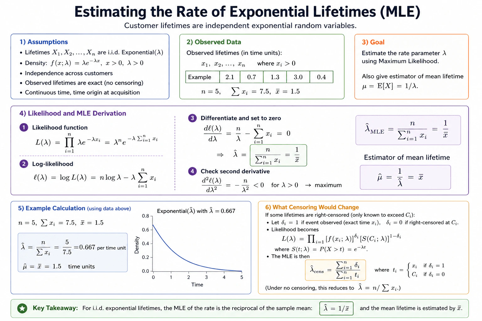
Customer lifetimes are independent exponential random variables. How would you estimate the rate parameter? diagram
How to Explain It in an Interview

The exponential probability density is f(x; λ) = λ exp(-λx) for x > 0 and λ > 0. Here λ is the unknown population rate parameter. Independence means the joint density of the observed lifetimes is the product of the individual densities.

For exact observations x1,...,xn, the likelihood is L(λ) = Π[i=1 to n] λ exp(-λxi) = λ^n exp(-λΣxi).

Probability describes possible data for a fixed parameter. Likelihood uses the observed data and views the same expression as a function of the unknown parameter λ.

It is easier to maximize the log-likelihood: ℓ(λ) = log L(λ) = n log λ - λΣxi.

Differentiate with respect to λ: dℓ/dλ = n/λ - Σxi.

Set this equal to zero: n/λ - Σxi = 0, so λ̂ = n/Σxi = 1/x̄, where x̄ = (1/n)Σxi is the sample mean lifetime.

The second derivative is d²ℓ/dλ² = -n/λ², which is negative for λ > 0. Therefore this stationary point is a maximum.

It is important to distinguish three ideas. λ is the unknown parameter. λ̂ = n/Σxi is the estimator, meaning the rule calculated from random sample data. After the lifetimes are observed, the resulting numerical value is an estimate. In the diagram example, n = 5, Σxi = 7.5 time units, and x̄ = 1.5 time units. Therefore λ̂ = 5/7.5 ≈ 0.667 per time unit.

For an exponential distribution, the population mean lifetime is μ = E[X] = 1/λ. By the invariance property of maximum likelihood, substituting λ̂ gives the MLE μ̂ = 1/λ̂ = x̄. In the same example, μ̂ = 1.5 time units.

Censoring changes the calculation. Suppose some lifetimes are right-censored, so for those customers we only know that their lifetime exceeds a censoring time Ci. Let δi = 1 when the event is observed and δi = 0 when it is right-censored. An observed event contributes the density f(xi; λ), while a censored observation contributes the survival probability S(Ci; λ) = P(X > Ci) = exp(-λCi). The likelihood becomes L(λ) = Π[i=1 to n] [f(xi; λ)]^δi [S(Ci; λ)]^(1-δi).

For this exponential model, define ti = xi when δi = 1 and ti = Ci when δi = 0. Maximizing the censored-data likelihood gives λ̂cens = (Σδi)/(Σti). The numerator is the number of observed events, and the denominator is total observed time at risk. When there is no censoring, every δi = 1 and ti = xi, so this reduces to λ̂ = n/Σxi. Therefore the reciprocal-of-the-sample-mean formula applies directly to the fully observed case, while censoring must be represented explicitly in the likelihood.

Technical Approach

1. Confirm that lifetimes are positive, measured in the same time units, and modeled as independent Exponential(λ) observations. 2. For fully observed data, write L(λ) = λ^n exp(-λΣxi). 3. Take logs to obtain ℓ(λ) = n log λ - λΣxi. 4. Differentiate and solve dℓ/dλ = 0, giving λ̂ = n/Σxi = 1/x̄. 5. Check that d²ℓ/dλ² = -n/λ² < 0. 6. Estimate mean lifetime with μ̂ = 1/λ̂ = x̄. 7. If observations are right-censored, replace censored density contributions with survival contributions and use λ̂cens = Σδi/Σti.

Practical Insights

For fully observed data, estimation only needs the number of lifetimes and their sum, so one pass through n observations takes O(n) time and O(1) extra memory. The formula is simple, but it depends on the exponential model being appropriate, including a constant event rate over time and independence across customers. Right-censored exponential data are also simple to summarize if event indicators and observed times are available, but ignoring censoring uses the wrong likelihood and can distort the rate estimate.

Why Interviewers Ask This

This question tests whether a candidate can move from a probability model to a likelihood, derive a maximum-likelihood estimator, distinguish the unknown parameter from its estimator and numerical estimate, interpret the result in the correct time units, and recognize how censoring changes the likelihood contribution of an observation.

Common interview mistakes

Common mistakes are using λ̂ = x̄ instead of its reciprocal, forgetting that the exponential mean is 1/λ, multiplying densities without stating independence, confusing likelihood with the probability that λ is true, failing to check that the stationary point is a maximum, mixing rate units with lifetime units, and treating right-censored observations as exact event times. For right censoring, censored cases contribute S(Ci; λ), not f(Ci; λ).

Interview tip

Start with the assumptions and density, derive the likelihood in one line, move to the log-likelihood, and show λ̂ = 1/x̄. Then state that mean lifetime is estimated by x̄. Finish by explaining that right censoring replaces density contributions with survival contributions and changes the numerator from n to the number of observed events.

Interviewer may ask next
What assumption of the exponential model is especially important for interpreting λ as one constant rate?

The exponential model has a constant hazard, or event rate, over time. In this question, customer lifetimes are also assumed independent and drawn from the same Exponential(λ) distribution. If the event rate systematically changes with elapsed lifetime, one common exponential rate may be a poor model even though the MLE derivation is correct under the stated exponential assumption.

How does the estimator change if some customer lifetimes are right-censored?

Let δi = 1 for an observed event and δi = 0 for a right-censored customer. An observed event contributes f(xi; λ) = λ exp(-λxi), while a customer censored at Ci contributes S(Ci; λ) = exp(-λCi). If ti equals xi for an observed event and Ci for a censored observation, maximizing the exponential likelihood gives λ̂cens = Σδi/Σti. Thus the numerator is the number of observed events and the denominator is total observed time at risk. With no censoring, this reduces to n/Σxi.

20. How do maximum-likelihood and maximum-a-posteriori estimation differ?Statistics And ProbabilityHard

Question Details

For a parameter θ, compare optimizing the likelihood p(data|θ) with optimizing the posterior p(θ|data). Show how a prior changes the objective, connect common priors to regularization without assuming they are always equivalent, and discuss asymptotic behavior, uncertainty, and cases where the MAP estimate is sensitive to parameterization.

Short Interview Answer (30-60 seconds)

MLE chooses the parameter that makes the observed data most likely. MAP uses the same likelihood but also includes a prior belief about the parameter. In log form, that prior becomes an added term that can resemble regularization. With enough data, MAP often approaches MLE under suitable conditions.

Detailed Explanation

Let D denote the observed data and θ the unknown parameter. MLE asks which θ makes D most likely under the model. MAP asks which θ is most plausible after combining the observed data with a prior distribution p(θ). The prior changes the optimization objective and can sometimes behave like a regularization penalty. The exact relationship depends on the likelihood, prior, parameterization, and scaling. MLE and MAP are both estimators that return point estimates, so neither point alone represents complete uncertainty. MAP also has an important sensitivity to how the parameter is represented.

Useful Questions to Ask the Interviewer
  1. Should I derive both objectives in log form?
  2. Would you like the Gaussian-prior-to-ridge and Laplace-prior-to-lasso examples?
  3. Should I discuss the regularity conditions needed for the large-sample comparison?
  4. Should I explain why MAP can change under reparameterization?
How do maximum-likelihood and maximum-a-posteriori estimation differ? diagram
How to Explain It in an Interview

Start with the objectives.

For maximum likelihood estimation,

θ̂_MLE = argmaxθ p(D|θ).

After D has been observed, p(D|θ) is treated as a function of θ. This is the likelihood. It is not a probability distribution over θ. Because the logarithm is increasing, maximizing the likelihood is equivalent to maximizing the log-likelihood:

θ̂_MLE = argmaxθ log p(D|θ).

For maximum a posteriori estimation, use Bayes' rule:

p(θ|D) = p(D|θ)p(θ) / p(D).

Here p(θ) is the prior density and p(θ|D) is the posterior density. The evidence p(D) does not depend on θ, so it does not change the maximizing value. Therefore,

θ̂_MAP = argmaxθ p(D|θ)p(θ),

and equivalently,

θ̂_MAP = argmaxθ [log p(D|θ) + log p(θ)].

This is the central difference: MLE optimizes only fit to the observed data, while MAP optimizes data fit plus the prior preference for parameter values.

The prior can sometimes create an objective that looks exactly like regularization. Consider linear regression with

y = Xθ + ε,

where y is the response vector, X is the design matrix, and ε ~ N(0, σ²I) is Gaussian observation noise with variance σ². If the prior is Gaussian,

θ ~ N(0, τ²I),

where τ² is the prior variance, the negative log-posterior is, up to constants,

(1 / 2σ²)||y - Xθ||²₂ + (1 / 2τ²)||θ||²₂.

This has the ridge-regression form. If the objective is rescaled so the squared-error coefficient is 1/2, the corresponding L2 penalty weight is λ = σ²/τ².

If instead the components of θ have an independent zero-centered Laplace prior with scale b, then the negative log-prior contributes

(1 / b)||θ||₁.

With the same Gaussian-noise regression likelihood, the MAP objective has the lasso form. Under the same rescaling, its L1 weight is proportional to σ²/b.

These examples do not mean every prior is equivalent to a familiar regularizer. The relationship comes from the negative log-prior, and its exact form depends on the model. A heavy-tailed prior such as a Student-t prior gives a different, non-L1 and non-L2 penalty and generally penalizes very large coefficients less aggressively than a Gaussian prior. A uniform prior on a bounded interval contributes a constant inside the allowed region and zero posterior density outside it, so it acts like a hard constraint rather than ordinary shrinkage.

For asymptotic behavior, suppose the sample size increases while the prior stays fixed. Under standard regularity conditions, such as an identifiable and well-specified model, a sufficiently regular likelihood, and a prior with positive density near the true parameter, the log-likelihood grows with the amount of data while the log-prior remains an order-one contribution. The data therefore dominate. In this setting, MAP and MLE typically have the same first-order limit and asymptotic distribution. This statement is not universal; irregular, non-identifiable, boundary, misspecified, or strongly constrained models can behave differently.

For uncertainty, both MLE and MAP return a single point estimate. MLE uncertainty may be estimated from likelihood curvature, Fisher-information-based large-sample approximations, profile likelihood, or bootstrap methods when their assumptions are appropriate. MAP is also only one point from a posterior distribution. A full Bayesian analysis keeps the complete posterior p(θ|D), which can be used to report posterior credible intervals and other uncertainty summaries.

Finally, MAP is generally sensitive to parameterization. Suppose φ = g(θ) is a one-to-one transformation. The transformed posterior density includes a Jacobian factor:

p(φ|D) = p(θ|D)|dθ/dφ|.

Because MAP chooses the location where a density is highest, this Jacobian can move the mode. Therefore the MAP obtained directly in φ-space need not equal g(θ̂_MAP). MLE is equivariant under a one-to-one reparameterization because the likelihood preserves the ordering of corresponding parameter points.

A strong interview summary is: MLE means data fit only. MAP means data fit plus prior information. Some priors produce familiar regularization objectives in specific models, but that connection is not universal. With enough informative data and standard regularity conditions, MAP often approaches MLE. Neither point estimate alone gives complete uncertainty, and MAP requires extra care because posterior modes depend on parameterization.

Technical Approach
  1. Define the observed data D and unknown parameter θ.
  2. Write MLE as θ̂_MLE = argmaxθ p(D|θ), or equivalently maximize log p(D|θ).
  3. Apply Bayes' rule for MAP and remove p(D) from the optimization because it does not depend on θ.
  4. Write MAP as θ̂_MAP = argmaxθ [log p(D|θ) + log p(θ)].
  5. Explain that the log-prior changes the objective by favoring some parameter values over others.
  6. Use the Gaussian-noise regression example to show that a Gaussian prior gives an L2-type ridge objective and a Laplace prior gives an L1-type lasso objective.
  7. State that other priors can produce different penalties or hard constraints, so the connection is not universally equivalent to standard regularization.
  8. Explain that a fixed prior often becomes less influential as the sample size grows under suitable regularity conditions.
  9. Separate point estimation from uncertainty: MLE and MAP each return one value, while a full posterior represents Bayesian uncertainty.
  10. Mention that MAP modes are generally not invariant to one-to-one reparameterization because posterior densities transform with a Jacobian.
Practical Insights

The computational cost of MAP can be close to MLE when the prior is easy to evaluate because MAP mainly adds a log-prior term to the same likelihood optimization. The larger tradeoff is statistical. A sensible prior can stabilize estimates when data are limited or parameters are weakly identified, but an unsuitable prior can pull the MAP estimate in an undesirable direction. With a large amount of informative data, the prior often has much less influence. Computing a full posterior is usually more expensive than finding one MLE or MAP point, but it gives much richer uncertainty information.

Why Interviewers Ask This

This question tests whether a candidate can distinguish likelihood from posterior probability, explain how prior information changes an estimation objective, connect priors to regularization without overgeneralizing, reason about asymptotic behavior and uncertainty, and recognize that posterior modes can depend on parameterization.

Common interview mistakes

Common mistakes include treating p(D|θ) as a probability distribution over θ instead of a likelihood; forgetting that MAP adds a prior term; saying MAP is the same thing as the full Bayesian posterior; claiming every Gaussian prior always means ridge or every Laplace prior always means lasso without specifying the likelihood and objective scaling; assuming every prior produces a standard L1 or L2 penalty; saying MAP and MLE always become identical with large data without stating regularity conditions; treating priors only as regularizers rather than probability models; claiming a heavy-tailed prior necessarily shrinks large coefficients more strongly than a Gaussian prior; and claiming MAP is invariant to one-to-one reparameterization.

Interview tip

Start with the two optimization equations. Then say that MAP adds a log-prior term to the log-likelihood. Use Gaussian-to-L2 and Laplace-to-L1 as model-specific examples, explicitly warn that the equivalence is not universal, and finish with large-sample behavior, uncertainty, and MAP's parameterization sensitivity.

Interviewer may ask next
Under what assumptions can MAP and MLE become similar as the sample size grows?

The result needs regularity conditions. A typical setting has an identifiable and well-specified model, a sufficiently regular likelihood, and a fixed proper prior that assigns positive density near the true parameter. As the sample size n grows, the log-likelihood usually grows on the order of n while the fixed log-prior remains on the order of one. The likelihood therefore dominates, so MAP and MLE typically converge to the same limiting parameter and have the same first-order asymptotic distribution. This conclusion can fail for irregular, non-identifiable, misspecified, boundary, constrained, or otherwise nonstandard models.

Why can MAP change after a one-to-one reparameterization while MLE transforms naturally?

MAP chooses the mode of a posterior density, and density height depends on the coordinate system. If φ = g(θ), the transformed posterior contains the Jacobian factor |dθ/dφ|. That factor can move the location of the highest density, so the MAP found directly in φ-space need not equal g(θ̂_MAP). Posterior probability mass still transforms consistently; the issue is specifically the density mode. For MLE, corresponding parameter values have the same likelihood ordering under a one-to-one transformation, so the transformed MLE is g(θ̂_MLE).

More questions load as you scroll

Disclaimer: This interview guide is for educational and informational purposes only. It is designed to help readers prepare, but it does not guarantee any interview result, hiring decision, offer, or outcome. Interview questions, hiring criteria, and preferred answers can vary by employer, interviewer, industry, location, and time. The examples and explanations reflect the authors' research and judgment, are provided without warranties of any kind, and should not be treated as the only correct approach. Diagrams are simplified illustrations intended to highlight the main components and their interactions; actual systems and implementations may be more complex. Alternative approaches may be equally valid or better suited to a particular question, context, or interviewer. To the fullest extent permitted by applicable law, the author, contributors, and publisher are not liable for decisions made, actions taken, or losses incurred based on this guide.

Content Accuracy and Verification: To the fullest extent permitted by applicable law, we do not represent or warrant that interview guides, questions, answers, examples, or diagrams are accurate, complete, current, error-free, or suitable for any particular purpose. You are responsible for independently reviewing and verifying the information before relying on it.