This interview guide is for educational and informational purposes only. It is designed to help readers prepare, but it does not guarantee any interview result, hiring decision, offer, or outcome. Interview questions, hiring criteria, and preferred answers can vary by employer, interviewer, industry, location, and time. All answers, examples, and explanations in this guide are suggested examples for interview preparation, not definitive answers or instructions for professional practice. They are based on research and judgment, are provided without warranties of any kind, and should be adapted to the question, role, and applicable laws and professional requirements. Diagrams are simplified illustrations intended to highlight the main concepts and their relationships; actual situations, systems, and practices may be more complex. Alternative approaches may be equally valid or better suited to a particular question, context, or interviewer. To the fullest extent permitted by applicable law, the contributors and publisher are not liable for decisions made, actions taken, or losses incurred based on this guide.
State Laws and Professional Responsibilities
Laws and requirements governing an occupation vary by state and jurisdiction. You are responsible for checking the current laws, licensing requirements, and scope-of-practice rules that apply to your location and role, and for ensuring that your answers and actions comply with them. Adapt examples in this guide to those requirements. This guide is not legal advice.
Identity, Image, and Privacy Notice
To respect individual privacy, some names, profile photographs, avatars, biographical details, and other identifying information displayed in this guide may be replaced with pseudonyms, licensed stock images, illustrative avatars, composite images, or representative descriptions. Unless a person is expressly identified as an actual contributor, a displayed name, image, or profile should not be understood as depicting or identifying a specific candidate, interviewer, employee, or other real individual. These representations are provided for editorial and illustrative purposes only and do not imply endorsement, employment, participation, or affiliation with this guide or any company mentioned in it. Any resemblance to an actual person is coincidental.
Company Notice
This guide is an independent educational resource and is not affiliated with, endorsed by, sponsored by, or approved by the company named in this guide. Company names identify reported interview experiences or the employer context of clearly labeled original practice exercises. Interview practices can change without notice, and inclusion of company-specific content does not mean these questions are official, complete, or guaranteed to be asked. To the fullest extent permitted by law, the author, contributors, and publisher are not responsible for outcomes related to use of this material.
Content Accuracy and Verification
To the fullest extent permitted by applicable law, we do not represent or warrant that interview guides, questions, answers, examples, or diagrams are accurate, complete, current, error-free, or suitable for any particular purpose. You are responsible for independently reviewing and verifying the information before relying on it.
Questions or comments?
Contact us for general questions, or share feedback, technical corrections, and comments with the community.
1. What is dimensional data modeling, and what are facts, dimensions, grain, and a star schema?Data ModelingEasy
i Question Details
Define dimensional modeling for analytical workloads. Explain that grain states what one fact row represents, facts measure events or states, dimensions provide descriptive context, and a star schema connects fact tables to dimensions. Contrast this purpose with normalized transactional modeling and introduce surrogate keys and slowly changing dimensions.
Short Interview Answer (30-60 seconds)
Dimensional modeling organizes analytical data into fact and dimension tables. Grain defines what one fact row represents, facts store measurements, and dimensions provide descriptive context. A star schema connects the fact table to surrounding dimensions. Surrogate keys identify dimension rows, while slowly changing dimensions manage attribute changes over time.
Detailed Explanation
This question asks how to arrange information so people can study activity clearly and consistently. The first decision is what one recorded row means. Then separate the values being measured from the descriptive information used to explain those values. The design should make it easy to look at results by different descriptions, such as category or time. You should also explain why this structure is different from systems built mainly to record day-to-day operations, and how descriptive information can either replace old values or keep earlier versions when changes happen.
Useful Questions to Ask the Interviewer
Do you want only the core concepts, or should I also explain common warehouse implementation practices?
Should I briefly explain the main slowly changing dimension types?
How to Explain It in an Interview
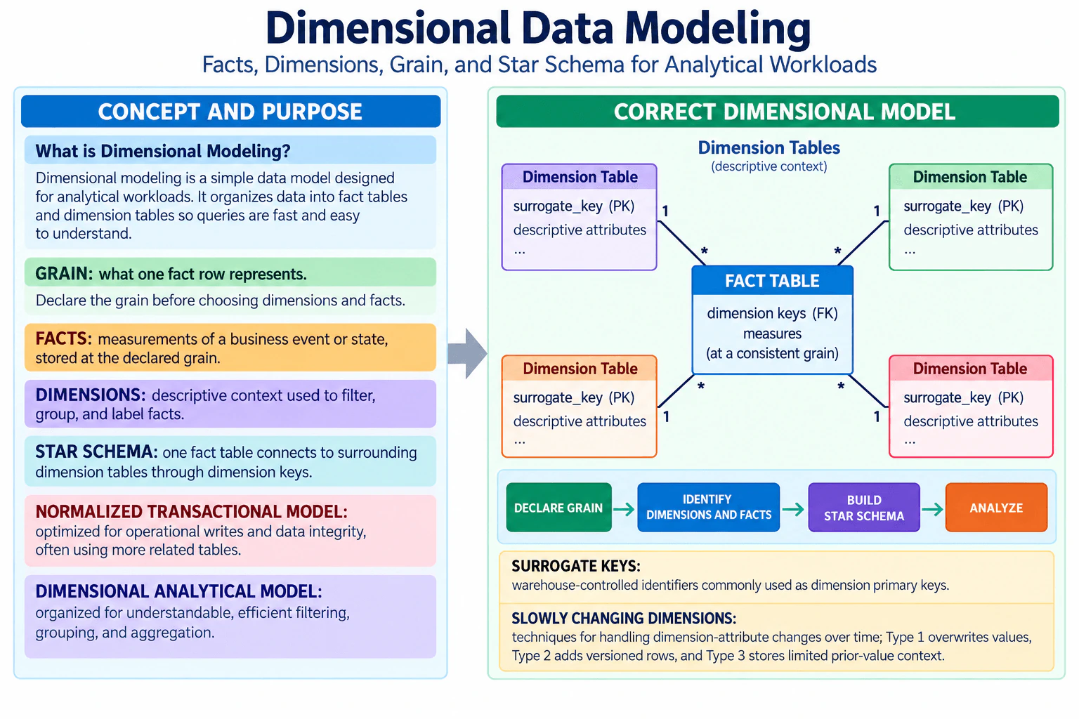
Start with the practical decision: declare the grain before choosing facts and dimensions. Grain means exactly what one row in the fact table represents. Every measurement in that fact table should be stored at that consistent level.
Facts are measurements of a business event or state stored at the declared grain. A fact table typically contains dimension keys and measures. Measures are the values analysts summarize, such as amounts, quantities, counts, balances, or other numeric observations.
Dimensions provide descriptive context. Their attributes are used to filter, group, and label facts. In the approved diagram, each dimension table contains a warehouse-controlled surrogate key as its primary key plus descriptive attributes. The central fact table contains the corresponding dimension keys as foreign keys.
A star schema places the fact table at the center and connects it directly to surrounding dimension tables. The relationships shown are one-to-many from each dimension to the fact table: one dimension row can be referenced by many fact rows.
The practical modeling flow shown in the diagram is: DECLARE GRAIN → IDENTIFY DIMENSIONS AND FACTS → BUILD STAR SCHEMA → ANALYZE. This order matters because the grain establishes the meaning of each fact row and therefore controls which facts and dimension relationships are valid.
Surrogate keys are warehouse-controlled identifiers commonly used as dimension primary keys. They separate warehouse identity from source-system natural keys and are especially useful when a dimension needs multiple historical versions.
Slowly changing dimensions, or SCDs, handle descriptive attribute changes over time. Type 1 overwrites the existing value, so prior history is not preserved. Type 2 creates a new versioned row, normally with a new surrogate key, so historical facts can remain associated with the correct dimension version. Type 3 keeps limited prior-value context in additional attributes.
The main tradeoff is purpose. A normalized transactional model is optimized for operational writes and data integrity and often uses more related tables. A dimensional analytical model is organized for understandable and efficient filtering, grouping, and aggregation. Neither approach is universally better; each is designed for a different workload.
Technical Approach
Declare the grain: state exactly what one fact row represents.
Identify the facts: choose measurements that belong at that grain.
Identify the dimensions: choose descriptive context used to filter, group, and label the facts.
Assign warehouse-controlled surrogate keys to dimensions where appropriate.
Build the star schema by placing dimension keys in the fact table and connecting the fact table directly to the surrounding dimensions.
Choose an appropriate slowly changing dimension strategy for descriptive attributes that change over time.
Validate that every fact remains at one consistent grain and that the model supports the intended analytical questions.
Practical Complexity & Trade-offs
There is no useful Big-O complexity for this conceptual modeling question. The important costs are data volume, storage, query work, load complexity, and maintenance. Fact tables can become very large because they store many events or states, while dimension tables are usually smaller. A star schema generally makes analytical queries easier to understand because facts connect directly to descriptive dimensions. Type 2 slowly changing dimensions require more storage and more loading logic because each historical version is stored as another dimension row.
Where it is used
Dimensional modeling is widely used in data warehouses, analytical data marts, reporting systems, business-intelligence platforms, and semantic models. It is useful when analysts need to summarize measurements and examine them by descriptive context. Typical uses include dashboards, historical reporting, trend analysis, financial analysis, operational analytics, and other read-heavy analytical workloads.
Why Interviewers Ask This
Interviewers want to know whether you understand the core structure of analytical data models and can connect grain, facts, dimensions, star-schema relationships, surrogate keys, and slowly changing dimensions into one coherent design. They also want to see whether you understand why analytical dimensional models and normalized transactional models serve different workloads.
Common interview mistakes
Common mistakes include choosing facts before declaring the grain, mixing multiple grains in one fact table, treating descriptive attributes as facts, reversing the one-to-many relationship between dimensions and facts, assuming every natural source key should also be the warehouse dimension key, and describing dimensional modeling as simply denormalization. Another mistake is saying Type 1 preserves history or that Type 2 only overwrites the current row. Also avoid claiming that dimensional modeling replaces normalized transactional modeling; they are designed for different workloads.
Interview tip
Present the answer as one connected sequence: declare the grain, identify facts and dimensions, connect them in a star schema, then explain surrogate keys and slowly changing dimensions. Finish by contrasting analytical and transactional modeling. This demonstrates both terminology and practical modeling judgment.
Interviewer may ask next
Why should you declare the grain before choosing facts and dimensions?
The grain defines exactly what one fact row represents, so it establishes the meaning of every measurement in that table. Once the grain is fixed, you can choose facts that are valid at that level and dimensions that describe the same event or state. If the grain is unclear or mixed, aggregations can become incorrect because different rows may represent different levels of detail.
When would you use a Type 1 slowly changing dimension instead of Type 2?
Use Type 1 when you only need the latest descriptive value and do not need historical versions, such as correcting an error or updating an attribute whose previous value is not analytically important. Use Type 2 when historical context matters. Type 2 creates versioned dimension rows so older facts can remain associated with the dimension attributes that were valid for that historical version.
2. What distinguishes a weak entity set from a strong entity set?Data ModelingEasy
i Question Details
Explain how the dependent entity is identified when its own attributes are insufficient to identify it independently.
Short Interview Answer (30-60 seconds)
A strong entity has its own key and can be identified independently. A weak entity cannot be uniquely identified by its own attributes alone. It needs its owner's key plus a partial key. Here, Dependent is identified by (student_id, dependent_name).
Detailed Explanation
A strong item can be recognized uniquely using information that belongs to it. A weak item cannot be recognized uniquely from its own information, so it must be connected to another item that owns it. In this example, each Student has its own unique identifier. A Dependent has a name, birth date, and relationship, but those details alone may not make it unique. Therefore, the Dependent is identified using the Student's identifier together with the Dependent's name. This also allows different students to have dependents with the same name without confusing their identities.
Useful Questions to Ask the Interviewer
Should I explain the distinction using Chen ER notation as well as the key relationship?
Should I show how the weak entity's partial key combines with the owner's primary key?
How to Explain It in an Interview
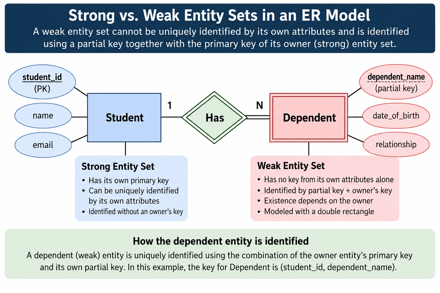
Start with identity. A strong entity set has a key that uniquely identifies each entity without using an owner's key. In the diagram, Student is the strong entity, and student_id is its primary key.
A weak entity set does not have a complete key formed only from its own attributes that is sufficient to identify each entity uniquely. It depends on an owner strong entity for identification. In the diagram, Dependent is the weak entity. dependent_name is a partial key: it can distinguish Dependents belonging to the same Student, but it is not globally sufficient by itself.
The identifying relationship is Has. One Student can have many Dependents, so the diagram shows a 1:N relationship. The Dependent side has total participation in the identifying relationship because a Dependent in this model must belong to an owning Student. In Chen-style notation, Dependent is therefore shown with a double rectangle, the identifying relationship Has with a double diamond, and the partial key dependent_name with a dashed underline.
The complete identifier for a Dependent is the combination (student_id, dependent_name). Two different Students can each have a Dependent with the same dependent_name because their student_id values are different. Within one Student, dependent_name must distinguish that Student's Dependents if it is used as the partial key.
The key distinction is about identification, not the number of attributes. A strong entity is identifiable using its own key. A weak entity requires the owner's key together with its partial key.
Technical Approach
Check whether the entity has a key that uniquely identifies it using only its own attributes.
If it does, model it as a strong entity set.
If its own attributes are insufficient, identify the owner strong entity.
Identify the weak entity's partial key, which distinguishes weak entities under the same owner.
Form the weak entity's complete identifier from the owner's primary key plus the partial key.
Model the identifying relationship and total participation of the weak entity consistently.
Time & Space Complexity
There is no meaningful algorithmic time or memory complexity for this conceptual ER-model question. The main cost is modeling and maintenance complexity. A weak entity carries the owner's key as part of its identity in the relational design, so the database must maintain that relationship and its referential integrity. This extra dependency is intentional because it accurately represents the weak entity's identity.
Where it is used
Weak entities are useful when a record's identity exists only within the context of an owner. Examples include a dependent belonging to a person, a line item identified within an order, or a numbered child record within a parent. In this diagram, Dependent belongs to Student and is identified by student_id together with dependent_name.
Why Interviewers Ask This
The interviewer wants to know whether you understand entity identity, ownership, keys, partial keys, and identifying relationships in an ER model. A strong answer explains both the difference between strong and weak entity sets and how the weak entity becomes uniquely identifiable through its owner.
Common interview mistakes
Common mistakes are saying that a weak entity has no attributes, saying that its partial key uniquely identifies it globally, or forgetting the owner's key. Another mistake is thinking that the difference is simply whether the entity can exist conceptually on its own. For this model, the important distinction is identification: dependent_name alone is not the complete identifier; the identifier is (student_id, dependent_name). It is also a mistake to omit the identifying relationship between Student and Dependent.
Interview tip
Lead with one sentence: a strong entity has its own complete key, while a weak entity needs its owner's key plus a partial key. Then use the diagram example: Student uses student_id, while Dependent uses (student_id, dependent_name).
Interviewer may ask next
What is a partial key in a weak entity set?
A partial key is an attribute or set of attributes that distinguishes weak entities belonging to the same owner but is not sufficient to identify them globally. In this diagram, dependent_name is the partial key. It becomes part of the complete identifier when combined with the owner's student_id, giving (student_id, dependent_name).
Can two different Students have Dependents with the same dependent_name?
Yes. dependent_name is only a partial key, so it needs to distinguish Dependents within one owning Student rather than across all Students. Two Students can therefore each have a Dependent with the same dependent_name because their student_id values differ, making the complete identifiers different.
3. When is a degenerate dimension appropriate?Data ModelingEasy
i Question Details
Use an invoice identifier to discuss whether it needs a separate dimension table and how its placement affects analytical grouping.
Short Interview Answer (30-60 seconds)
Use a degenerate dimension when a transaction identifier is analytically useful but has no descriptive attributes of its own. Keep invoice_id directly in the line-level fact table so related invoice rows can be grouped into invoice-level totals without creating a separate invoice dimension.
Detailed Explanation
An invoice can contain several purchased items. Each item is stored as its own row, while all rows from the same invoice share the same invoice number. If that number only identifies which rows belong together and has no extra information of its own, another table adds little value. Keeping the invoice number on each item row lets analysts collect all rows for one invoice and calculate values such as the invoice total or number of lines. A separate table becomes useful only when the invoice itself has additional information that people need to analyze.
Useful Questions to Ask the Interviewer
Does the invoice identifier have any descriptive attributes that need to be analyzed independently?
Is the fact-table grain one row per invoice line item?
Should invoice-level metrics such as invoice total and line count be derived by grouping the line-level fact rows?
How to Explain It in an Interview
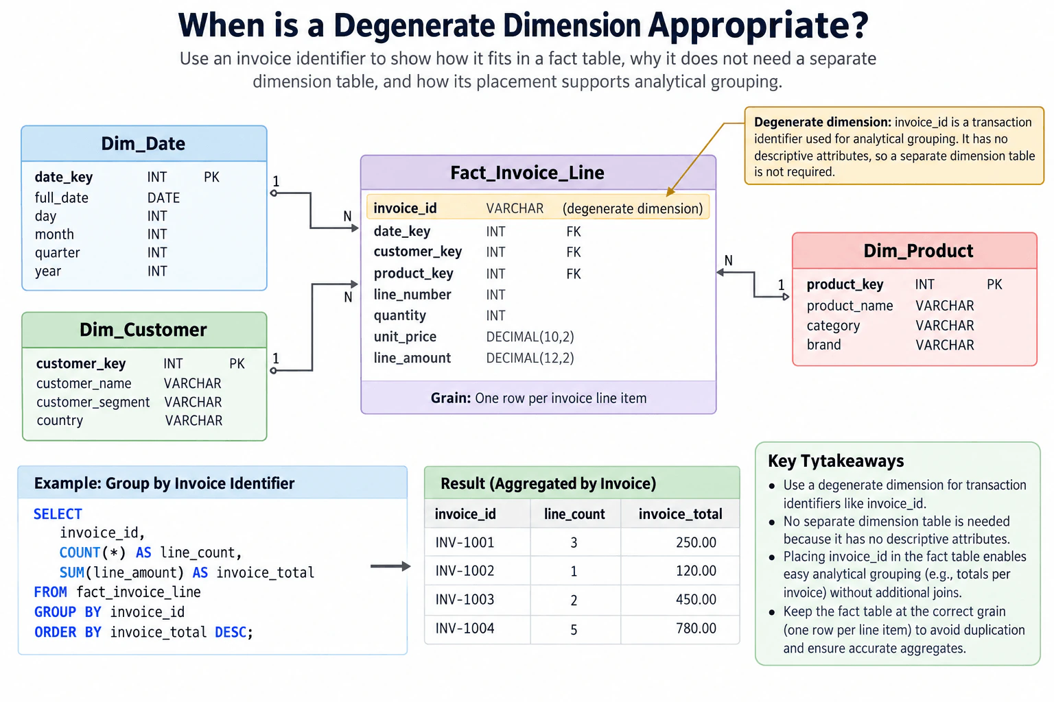
A degenerate dimension is a dimension identifier stored directly in a fact table without a separate dimension table. In the approved model, Fact_Invoice_Line has a grain of one row per invoice line item. It contains invoice_id as the degenerate dimension, plus date_key, customer_key, and product_key as foreign keys to Dim_Date, Dim_Customer, and Dim_Product.
The fact table also contains line-level data such as line_number, quantity, unit_price, and line_amount. Because the table is at invoice-line grain, one invoice can legitimately produce several fact rows. The same invoice_id therefore appears on every line belonging to that invoice. That repetition is intentional and does not mean the fact rows are accidental duplicates.
The decision is based on whether invoice_id has descriptive attributes of its own. In this design it does not, so a separate Dim_Invoice table would add an extra table and join without adding descriptive context. Storing invoice_id directly in Fact_Invoice_Line keeps the transaction identifier available for analysis.
The diagram shows invoice-level grouping directly from the fact table. Conceptually, the query groups by invoice_id, counts the line rows with COUNT(*), and sums line_amount with SUM(line_amount). The result grain changes from one row per invoice line item to one row per invoice. For example, INV-1001 is shown with 3 lines and an invoice total of 250.00; INV-1002 has 1 line and 120.00; INV-1003 has 2 lines and 450.00; and INV-1004 has 5 lines and 780.00.
The main tradeoff is future descriptive data. If the business later needs meaningful invoice-level attributes that are not already represented by other dimensions, then a separate invoice dimension may become appropriate. With the model shown here, however, invoice_id is only a transaction identifier used to group line-level facts, so a degenerate dimension is the simpler fit.
Technical Approach
Declare the fact-table grain as one row per invoice line item.
Identify invoice_id as the transaction identifier shared by all lines of one invoice.
Check whether the invoice identifier has descriptive attributes that justify its own dimension table.
If it has none, store invoice_id directly in Fact_Invoice_Line as a degenerate dimension.
For invoice-level analysis, group fact rows by invoice_id, count the line rows, and sum line_amount.
Reconsider a separate invoice dimension only if meaningful invoice-level descriptive attributes are later required.
Practical Complexity & Trade-offs
This design avoids maintaining and joining to a separate invoice dimension that would contain only identifiers. Storage still repeats invoice_id on each invoice-line row, which is expected at this grain. Invoice-level queries must group the relevant fact rows by invoice_id, so the work mainly depends on how many fact rows are read and aggregated. The important maintenance cost is keeping the declared grain clear so repeated invoice identifiers are not mistaken for duplicate fact rows.
Where it is used
This pattern is commonly used in dimensional warehouses for operational transaction identifiers that are useful for grouping but have no descriptive attributes of their own. Typical examples include invoice numbers, order numbers, ticket numbers, and similar identifiers stored in transaction-grain fact tables.
Why Interviewers Ask This
This question tests whether the candidate understands dimensional-modeling grain, can distinguish a transaction identifier from a normal dimension with descriptive attributes, and can avoid creating an unnecessary dimension table while still supporting correct analytical grouping.
Common interview mistakes
A common mistake is creating a separate invoice dimension that contains only invoice_id even though there are no descriptive invoice attributes. Another is assuming invoice_id must be unique in Fact_Invoice_Line; at one row per invoice line item, the same invoice_id correctly appears on multiple rows. A third mistake is forgetting the change in analytical grain: grouping by invoice_id produces one result row per invoice, while the source fact table remains one row per invoice line item. Finally, if meaningful invoice-level descriptive attributes are later introduced, continuing to treat the identifier as the only invoice representation may no longer be the best model.
Interview tip
State the fact grain first. Then give the decision rule: if the transaction identifier is useful for analysis but has no descriptive attributes, keep it in the fact table as a degenerate dimension. Use invoice_id to show how multiple invoice-line rows can be grouped into invoice-level totals without a separate invoice dimension.
Interviewer may ask next
Why is invoice_id allowed to repeat in the fact table?
Because Fact_Invoice_Line has a grain of one row per invoice line item, not one row per invoice. One invoice can contain several line items, so every line belonging to that invoice carries the same invoice_id. The repetition is intentional and lets analysts group those line rows back to the invoice level.
When would you create a separate invoice dimension instead of keeping invoice_id as a degenerate dimension?
Create a separate invoice dimension when the invoice has meaningful descriptive attributes that analysts need to filter, group, or report on as properties of the invoice itself. If invoice_id is only the transaction identifier, the separate dimension adds little value. Once real invoice-level descriptive context is required, a normal dimension can become justified.
4. How can a fact table represent events without numeric measures?Data ModelingEasy
i Question Details
Explain factless modeling for event attendance and for coverage analysis that identifies eligible events which never occurred.
Short Interview Answer (30-60 seconds)
A factless fact table stores dimension keys instead of numeric measures. One attendance row means an attendee attended an event. A separate coverage fact records eligible events, and a left join plus a null check finds eligible events that have no matching attendance.
Sometimes the important information is simply whether something happened, not how much of something happened. For example, you may only need to know that one person attended one event. You can save that occurrence directly instead of inventing a number such as 1. You may also keep a separate list of events that were allowed or expected to happen. Comparing that list with what actually happened lets you find events that were eligible but had no attendance. This gives a simple way to analyze both activity and missing activity.
Useful Questions to Ask the Interviewer
Is an eligible event represented only once, or can the same event have multiple eligible opportunities?
Should attendance allow only one row per attendee and event, as shown in the model?
Do you want the coverage query to return only event details, or would eligibility eventually depend on additional dimensions?
How to Explain It in an Interview
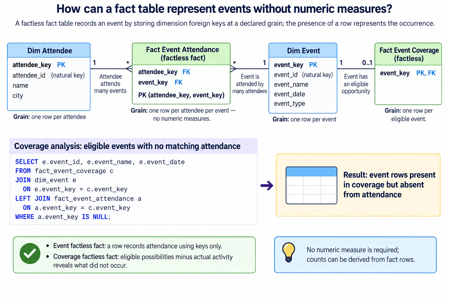
A factless fact table is a fact table whose rows represent business events or conditions without storing numeric measures. The important idea is the declared grain, which defines exactly what one row means.
In this model, Fact Event Attendance has the grain one row per attendee per event. It contains attendee_key and event_key, both foreign keys. Its composite primary key is (attendee_key, event_key), so the same attendee-event combination cannot be stored twice. The presence of a row means that attendance occurred. No numeric measure such as attendance_count = 1 is necessary because counts can be derived from fact rows.
Dim Attendee has one row per attendee. One attendee can relate to many attendance rows. Dim Event has one row per event, and one event can relate to many attendance rows because many attendees may attend the same event.
Coverage analysis answers a different question: what was eligible to happen but did not happen? The diagram uses a second factless table, Fact Event Coverage. Its grain is one row per eligible event. It contains event_key, which is both its primary key and a foreign key to Dim Event. With this displayed grain, an event has zero or one coverage row.
To find eligible events with no matching attendance, start from Fact Event Coverage, join to Dim Event to obtain the event attributes, and then left join to Fact Event Attendance using event_key. A left join preserves every eligible coverage row even when no attendance row matches. The condition a.event_key IS NULL then keeps only eligible events for which no attendance row exists.
Because event_key is a required key in the attendance fact, a null on the attendance side is the null introduced by the outer join and therefore means that no attendance match was found. The result is one row per eligible event with no matching attendance. The query has no ORDER BY, so the database does not guarantee result ordering.
The main tradeoff is that the coverage grain must match the real business meaning. The diagram is correct when eligibility is one condition per event. If eligibility later depends on attendee, date, location, or another dimension, those keys must become part of the coverage fact's grain; otherwise valid eligibility combinations would be lost.
Technical Approach
Declare the grain of each factless fact before choosing its keys.
Record actual attendance in Fact Event Attendance at one row per (attendee_key, event_key).
Record eligible opportunities in Fact Event Coverage at one row per eligible event_key.
Join coverage to Dim Event to return event attributes.
Left join coverage to attendance on event_key.
Keep rows where a.event_key IS NULL; these are eligible events with no matching attendance.
Derive counts by counting fact rows rather than storing a constant numeric measure.
Practical Complexity & Trade-offs
The attendance fact grows with the number of attendee-event occurrences, while the coverage fact grows with the number of eligible events. The coverage query must compare eligible events with attendance data, so runtime depends on table sizes and the database's chosen join plan. The SQL does not assume a particular physical execution strategy. Storage stays simple because the fact tables mainly contain keys. Maintenance remains straightforward as long as the declared grain continues to match the real business rule.
Example
The query begins with Fact Event Coverage, so every starting row represents an eligible event. It joins Dim Event to return event_id, event_name, and event_date. It then left joins Fact Event Attendance on event_key. The left join retains an eligible event when no attendance exists. Filtering with a.event_key IS NULL keeps exactly those unmatched coverage rows. Because Fact Event Coverage.event_key is its primary key, the result grain is one row per eligible event with no matching attendance. No ORDER BY is present, so result ordering is unspecified.
Code
-- Start from coverage: each row represents one eligible event.-- Because event_key is the coverage primary key, the starting grain is one row per eligible event.SELECT
e.event_id,
e.event_name,
e.event_date
FROM
fact_event_coverage AS c
-- Join the event dimension to return descriptive attributes for each eligible event.JOIN dim_event AS e ON e.event_key = c.event_key
-- Preserve every eligible event while looking for actual attendance rows.-- An event may have many attendance rows, but only events with zero matches survive the null filter.LEFTJOIN fact_event_attendance AS a ON a.event_key = c.event_key
-- A null attendance key here is introduced by the outer join when no attendance row matched.-- The final result grain is one row per eligible event with no matching attendance.WHERE
a.event_key ISNULL;
Where it is used
This pattern is useful for event attendance, registrations, student-course participation, account-event participation, promotion eligibility, scheduled-service coverage, and similar analytics where the occurrence or eligibility itself is the fact. It is especially useful when analysts need to count what happened and also identify eligible situations where no corresponding activity occurred.
Why Interviewers Ask This
This tests whether the candidate understands that a fact table does not need a numeric measure, can declare the correct grain, can distinguish actual activity from eligible coverage, and can use missing matches correctly. It also checks reasoning about keys, cardinality, duplicate prevention, joins, and null handling without inventing an artificial measure.
Common interview mistakes
Common mistakes are adding a fake numeric value such as 1 even though row presence already represents the event; failing to declare the attendance grain; allowing duplicate (attendee_key, event_key) rows and then overcounting; using an inner join for coverage analysis, which removes events with no attendance; checking a nullable descriptive attribute instead of the attendance key; treating eligibility only as an event attribute instead of a separate coverage condition; or keeping coverage at one row per event when eligibility actually varies by attendee, date, location, or another dimension.
Interview tip
Lead with the grain: say that a fact table does not need a numeric measure because the row itself can represent the fact. Then separate the two uses: attendance records what happened, while coverage records what was eligible to happen. Finish with the left join and null check that finds eligible events with no attendance.
Interviewer may ask next
How would you count attendees for each event if the fact table has no numeric measure?
Group Fact Event Attendance by event_key and use COUNT(*). Because the composite primary key allows at most one row for each (attendee_key, event_key) combination, each fact row represents one attendee-event occurrence. A stored constant measure such as 1 is unnecessary.
What changes if eligibility is per attendee and event instead of only per event?
The coverage grain must change to one row per eligible attendee per event. Fact Event Coverage would then include both attendee_key and event_key, normally with a composite key that prevents duplicate eligibility combinations. Coverage analysis would anti-match attendance using both keys. Keeping only event_key would lose which attendees were eligible.
5. Why maintain a dedicated calendar dimension?Data ModelingEasy
i Question Details
Discuss shared fiscal periods, holidays, and weekday attributes instead of independently deriving calendar rules in every report.
Short Interview Answer (30-60 seconds)
A dedicated calendar dimension defines fiscal periods, holidays, weekdays, and related date attributes once. Fact rows join to it by date, so every report uses the same rules. This reduces duplicated date logic, makes business-calendar changes easier to maintain, and produces consistent time-based analysis.
A company often needs many reports that organize information by date. Problems appear when every report decides for itself which dates belong to a business period, which days are holidays, or which days count as weekends. Two reports can then give different answers for the same business question. A shared calendar table keeps those decisions in one place. Reports reuse the same definitions instead of rebuilding them. When a rule changes, it can be updated centrally, making reports easier to maintain and their results easier to compare.
Useful Questions to Ask the Interviewer
Does the business use fiscal periods that differ from normal calendar months or quarters?
Are holiday and working-day rules shared across the organization, or can they vary by region or business unit?
Should multiple fact tables reuse this same calendar dimension as a shared dimension?
How to Explain It in an Interview
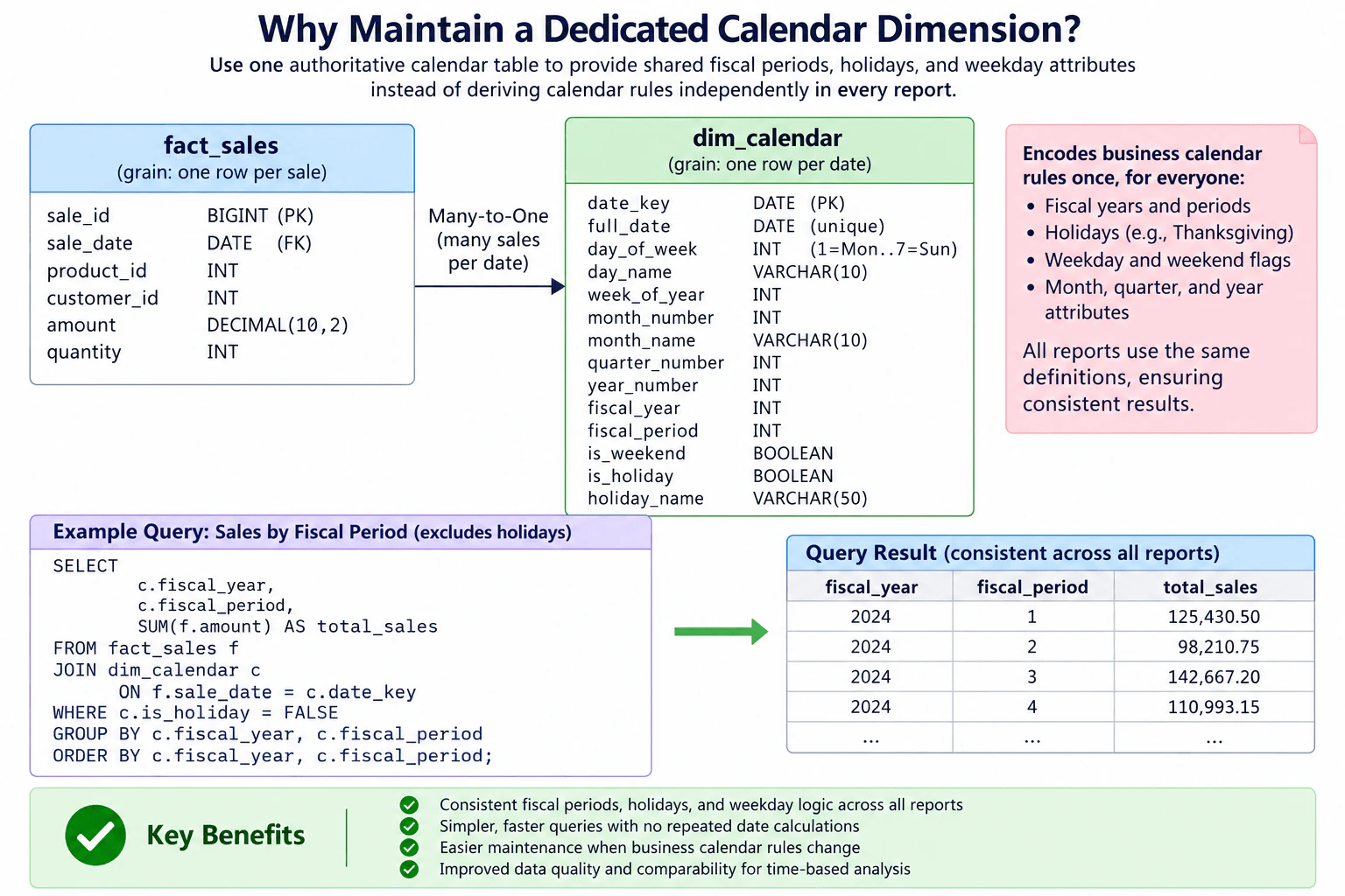
A calendar dimension is a dimension table with one row per calendar date. In the diagram, dim_calendar has that grain and uses date_key as its primary key. It also contains full_date as a unique date value and reusable attributes such as day_of_week, day_name, week_of_year, month_number, month_name, quarter_number, year_number, fiscal_year, fiscal_period, is_weekend, is_holiday, and holiday_name.
The fact_sales table has a different grain: one row per sale. Its sale_date is a foreign key to dim_calendar.date_key. Many sales can occur on the same date, so the relationship from fact_sales to dim_calendar is many-to-one.
The main reason to maintain the calendar dimension is consistency. Fiscal years, fiscal periods, holidays, weekdays, weekends, months, quarters, and years are encoded once. Reports look up those shared attributes instead of independently calculating calendar rules. That avoids subtle differences between reports and gives users one governed definition of time-based business concepts.
It also improves maintainability. If a fiscal-period mapping or holiday definition changes, the shared calendar data can be maintained centrally rather than changing similar logic in many reports. When multiple analytical processes use the same calendar definitions, the table can act as a conformed dimension shared across those processes.
The diagram's example joins fact_sales to dim_calendar with f.sale_date = c.date_key. It filters to dates where c.is_holiday = FALSE, groups by c.fiscal_year and c.fiscal_period, and calculates SUM(f.amount). The resulting grain is one row per fiscal-year and fiscal-period combination. The ORDER BY on those two columns gives a deterministic presentation order for the grouped result.
There are tradeoffs. The calendar dimension must contain every date required by the facts, and its business rules must be governed carefully because many reports can depend on them. A single is_holiday flag is only appropriate when that holiday definition is truly shared. If holiday rules vary by region, the model should represent that difference explicitly. A calendar dimension also avoids repeated date calculations and can simplify queries, but it does not guarantee faster execution on every database engine.
Technical Approach
Declare dim_calendar at one row per calendar date.
Store the shared fiscal, holiday, weekday, weekend, month, quarter, and year attributes in that dimension.
Keep fact_sales at one row per sale and reference the calendar through sale_date to date_key.
Join facts to the calendar instead of deriving business calendar rules independently in each report.
Filter, group, and report using the shared calendar attributes, such as excluding holidays and grouping by fiscal year and fiscal period.
Maintain calendar-rule changes centrally so dependent reports continue to use the same definitions.
Practical Complexity & Trade-offs
The calendar dimension is usually small because it stores only one row per date. The fact table still contains the much larger business data. Reports add a date lookup to the calendar table, but they avoid repeating fiscal, holiday, and weekday calculations in many places. The main savings are simpler report logic and lower maintenance effort. Query performance can vary by database engine, data size, statistics, indexes or physical layout, and execution plan, so the model should not be described as an automatic performance improvement.
Example
The SQL follows the diagram exactly. fact_sales remains at one row per sale, while dim_calendar remains at one row per date. The inner join maps each sale to its calendar row through sale_date = date_key. The holiday filter keeps only rows explicitly marked as non-holidays. Grouping by fiscal year and fiscal period changes the output grain to one row per fiscal-year and fiscal-period combination. The final ordering gives a deterministic display order.
Code
-- fact_sales grain: one row per sale.-- dim_calendar grain: one row per calendar date.-- Join each sale to the shared calendar row for its sale date.SELECT
c.fiscal_year,
c.fiscal_period,
-- Aggregate sales at the final grain: one row per fiscal year and fiscal period.SUM(f.amount) AS total_sales
FROM
fact_sales AS f
JOIN dim_calendar AS c ON f.sale_date = c.date_key
-- Keep only dates explicitly marked as non-holidays.-- If is_holiday is NULL, '= FALSE' is not true, so that row is excluded.WHERE
c.is_holiday =FALSEGROUPBY
c.fiscal_year,
c.fiscal_period
-- Return the grouped periods in deterministic fiscal order.ORDERBY
c.fiscal_year,
c.fiscal_period;
Where it is used
This approach is common in analytical warehouses, dimensional models, reporting systems, and semantic layers that need shared fiscal calendars, holiday analysis, weekday-versus-weekend reporting, month and quarter summaries, and consistent time filters across dashboards or multiple fact tables.
Why Interviewers Ask This
Interviewers want to know whether you understand why shared business calendar definitions should be modeled once instead of recreated independently in reports. A strong answer explains the calendar dimension grain, its many-to-one relationship with fact rows, shared fiscal and holiday logic, simpler reporting, centralized maintenance, and consistent analytical results.
Common interview mistakes
Common mistakes are calculating fiscal periods independently in every report, duplicating holiday logic, assuming calendar quarters always equal fiscal quarters, copying descriptive date attributes into the fact table, or creating separate incompatible calendar tables where one shared definition is required. Another mistake is claiming that a calendar dimension always makes queries faster. Its primary benefits are consistency, reuse, governance, simpler reporting logic, and centralized maintenance.
Interview tip
Lead with the practical reason: define business calendar rules once and reuse them everywhere. Then state the grains and relationship: one calendar row per date and many sales per date. Finish with consistency, easier maintenance, and the need to model regional or business-specific calendar differences explicitly when they exist.
Interviewer may ask next
Why not calculate fiscal periods, holidays, and weekdays directly from the sale date in every query?
Some simple calendar properties can be derived from a date, but business calendars often contain rules that are not captured by generic date functions. Fiscal periods may not match calendar months, and holidays are business-defined data. Repeating these rules in many reports also creates duplication and inconsistency. A dedicated calendar dimension stores the approved definitions once so every report can reuse them.
What if different regions use different holiday calendars?
Do not use one universal is_holiday value if the business meaning actually varies by region. Model the variation explicitly, for example with region-specific calendar attributes or another structure keyed by date and region. The same principle still applies: define each approved business calendar centrally rather than recreating holiday rules independently in every report.
6. What naming conventions would you establish for a data model?Data ModelingEasy
i Question Details
Address consistent table and column names, case, abbreviations, and recognizable key references.
Short Interview Answer (30-60 seconds)
I would use one documented convention: lowercase snake_case, descriptive fact_ and dim_ table prefixes, clear column names, limited well-known abbreviations, and consistent key references. For example, customer_id and date_key should keep the same names in the related fact and dimension tables.
Detailed Explanation
The goal is to give every part of the model a clear and predictable name so people can understand it without guessing. I would choose one writing style and use it everywhere, give groups and individual values descriptive names, avoid shortened words that may confuse readers, and make related identifiers easy to recognize. In the example, sales, date, customer, product, and store information all follow the same naming pattern. The exact words can differ between organizations, but the important rule is consistency because it makes the model easier to read, maintain, and use.
Useful Questions to Ask the Interviewer
Does the organization already have a naming standard that new data models must follow?
Should analytical tables use role prefixes such as fact_ and dim_?
Are there approved abbreviations or business terms that must be used consistently?
Should foreign-key columns normally keep the same names as the referenced keys?
How to Explain It in an Interview
I would define a small set of naming rules, document them, and apply them consistently across the model.
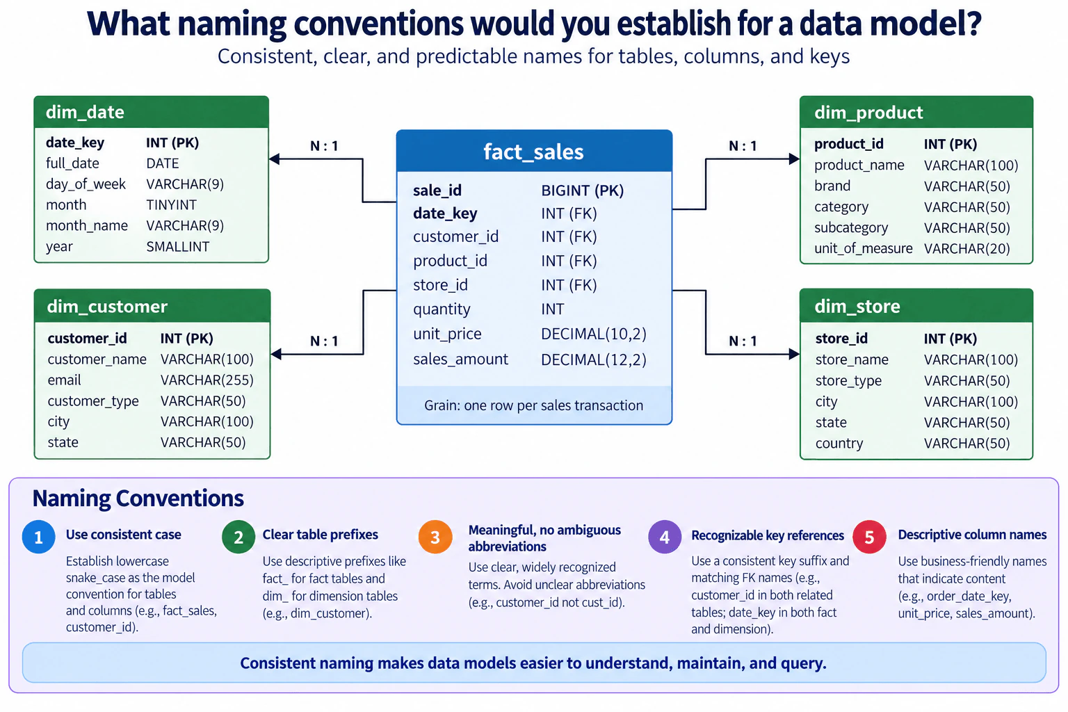
Use one case and separator style. In this model, I would establish lowercase snake_case for both table and column names. Examples include fact_sales, dim_customer, customer_id, unit_price, and sales_amount. I would describe this as the model's naming convention rather than as a universal SQL requirement.
Make table roles recognizable. The diagram uses fact_ for the central fact table and dim_ for dimensions: fact_sales, dim_date, dim_customer, dim_product, and dim_store. The prefixes let a reader recognize the analytical role of each table immediately.
Use descriptive column names. Examples in the diagram include customer_name, product_name, store_type, unit_price, sales_amount, full_date, day_of_week, month_name, and unit_of_measure. I would avoid vague names such as value or data when a more specific business name is available.
Limit abbreviations. I would use only abbreviations that are widely understood and consistently approved by the team. For example, id is recognizable in customer_id, product_id, and store_id. I would avoid unclear custom abbreviations such as cust_id when customer_id is easier to understand.
Make key references recognizable. Related keys should normally use the same visible name on both sides of a relationship. In the diagram, fact_sales.date_key references dim_date.date_key, fact_sales.customer_id references dim_customer.customer_id, fact_sales.product_id references dim_product.product_id, and fact_sales.store_id references dim_store.store_id. Each relationship is N:1 from fact_sales to its dimension: many sales rows can reference one date, customer, product, or store row.
The diagram declares fact_sales at a grain of one row per sales transaction. Its primary key is sale_id. Its foreign keys are date_key, customer_id, product_id, and store_id. Its remaining fields include quantity, unit_price, and sales_amount. The dimensions keep descriptive attributes under clear names. The main tradeoff is consistency versus local preference: different organizations may choose different conventions, but mixing conventions inside one model makes relationships and business meaning harder to recognize.
Technical Approach
Check whether an existing organizational naming standard already applies.
Choose one case and separator convention, such as lowercase snake_case.
Define recognizable table-role patterns where useful, such as fact_ and dim_.
Require descriptive column names.
Restrict abbreviations to approved, widely understood terms.
Keep related key names consistent where the relationship role is the same.
Document the convention and apply it during model reviews.
Practical Complexity & Trade-offs
Naming conventions add almost no query-time or memory cost. Their cost is mainly organizational: teams must agree on the rules, document them, review new models, and sometimes rename older objects. The benefit is lower maintenance effort because people spend less time interpreting table roles, column meanings, and relationships.
Where it is used
These conventions are useful in analytical warehouses, dimensional models, reporting layers, shared data marts, and other environments where engineers and analysts repeatedly read and join the same schemas. They are especially helpful in star-style models like the diagram, where a central fact table references several dimensions.
Why Interviewers Ask This
Interviewers want to know whether I can create a data model that engineers and analysts can understand quickly and maintain consistently. Good naming reduces ambiguity, makes table roles and relationships recognizable, and prevents teams from using different names for the same concepts.
Common interview mistakes
Common mistakes include mixing snake_case, camelCase, and other styles in one model; using inconsistent table-role names; creating vague columns such as value or data; inventing unclear abbreviations; changing the name of the same key unnecessarily across related tables; and treating a preferred naming convention as a universal database rule instead of a documented team standard.
Interview tip
Start with consistency, then give four concrete areas: table and column names, case, abbreviations, and key references. Use examples from the model such as fact_sales, dim_customer, customer_id, and date_key. Also mention that you would follow an existing organizational standard before creating a new one.
Interviewer may ask next
Would you always require a foreign key to have exactly the same name as the referenced key?
Normally, yes, when the relationship has the same business role because matching names make the reference easy to recognize. That is why the diagram uses customer_id, product_id, store_id, and date_key on both sides of their relationships. I would use a role-specific name only when the role itself must be distinguished, such as separate order_date_key and ship_date_key references to the same date dimension, and I would document that pattern.
Are fact_ and dim_ prefixes always required?
No. They are a naming convention, not a universal rule. In this diagram they are useful because fact_sales is clearly distinguished from dim_date, dim_customer, dim_product, and dim_store. If an organization already uses another clear convention, I would follow it. The important point is that table roles remain recognizable and the convention is applied consistently.
7. How should a star schema represent a multivalued dimension?Data ModelingMedium
i Question Details
Use the patient–diagnosis relationship to discuss bridge-table keys and the aggregation risk when one patient has several diagnoses.
Short Interview Answer (30-60 seconds)
Keep one fact row per encounter and store diagnosis_group_key in the fact. A bridge maps that group key to multiple diagnosis_key values. Because the bridge fans out fact rows, use distinct counts where appropriate and an explicit allocation or primary-diagnosis rule for additive measures.
A patient visit can have several diagnoses at the same time. The goal is to store all of those diagnoses without copying the visit itself several times. The model should keep one visit as one record while still allowing reports to find every diagnosis connected to it. The main risk is that, after joining the visit to several diagnoses, the same visit can appear several times. If a report simply adds values from those repeated rows, totals can become too large. The design therefore needs a safe way to connect diagnoses and clear rules for counting or allocating values.
Useful Questions to Ask the Interviewer
Is the fact grain one row per patient encounter, as shown in the diagram?
Should additive measures such as charge_amount be split across diagnoses, assigned only to a primary diagnosis, or intentionally attributed in full to each diagnosis?
Do reports need only per-diagnosis patient counts, or must totals also remain additive when users combine diagnosis groups or categories?
How to Explain It in an Interview
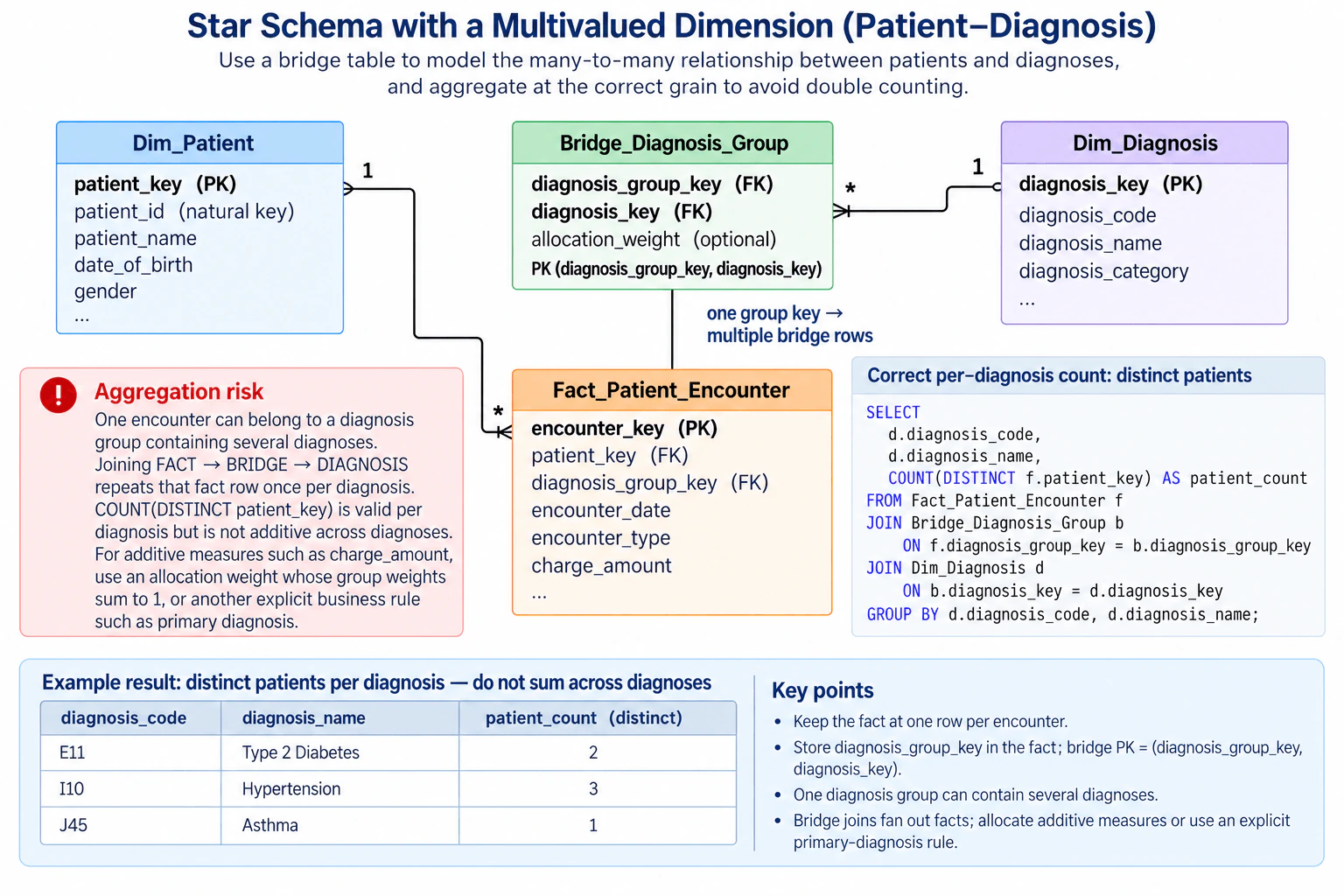
Start with the grain. Fact_Patient_Encounter has one row per encounter. Its primary key is encounter_key. patient_key is a foreign key to Dim_Patient, and diagnosis_group_key represents the set of diagnoses associated with that encounter.
Use Bridge_Diagnosis_Group to model the multivalued diagnosis relationship. Its composite primary key is (diagnosis_group_key, diagnosis_key). A single diagnosis_group_key can therefore map to several diagnosis_key values. Each bridge row represents one diagnosis that belongs to that group.
The bridge joins to Dim_Diagnosis by diagnosis_key. Dim_Diagnosis contains the diagnosis-level descriptive attributes shown in the diagram, including diagnosis_code, diagnosis_name, and diagnosis_category.
This design preserves the fact grain. One encounter still appears once in Fact_Patient_Encounter even when that encounter has several diagnoses. The fact does not need diagnosis_1, diagnosis_2, diagnosis_3 columns, and it does not need to duplicate the encounter row for every diagnosis.
The important tradeoff is fan-out. When a query follows Fact_Patient_Encounter → Bridge_Diagnosis_Group → Dim_Diagnosis, one encounter row is matched to one bridge row for each diagnosis in its group. That expansion is correct for analyzing the encounter by diagnosis, but it can make aggregates misleading.
For the diagram's example, COUNT(DISTINCT f.patient_key) grouped by diagnosis returns the number of distinct patients associated with each diagnosis. The result is one row per diagnosis code and name. These per-diagnosis patient counts are not additive across diagnoses because the same patient may have more than one diagnosis. That is why the example explicitly says not to sum those counts across diagnoses.
Additive fact measures need a separate business rule. If an encounter has charge_amount = 100 and its diagnosis group contains three diagnoses, a plain SUM(f.charge_amount) after crossing the bridge can associate that same 100 with all three diagnosis rows. If the business wants allocated diagnosis-level totals, use allocation_weight in the bridge and define weights so the members of a diagnosis group allocate the measure according to the agreed rule, such as weights summing to 1. Another valid option is an explicit primary-diagnosis rule when the business wants the full measure attributed to only one diagnosis.
No database dialect or version is specified, so the SQL example uses portable relational constructs rather than engine-specific syntax. It joins the fact to the bridge on diagnosis_group_key, joins the bridge to Dim_Diagnosis on diagnosis_key, and groups by diagnosis_code and diagnosis_name. No ORDER BY is shown because the question does not require deterministic output ordering.
The core interview answer is: preserve the natural encounter grain, use a bridge keyed by diagnosis_group_key and diagnosis_key for the multivalued dimension, and define aggregation semantics before users sum measures across the bridge.
Technical Approach
Declare the fact grain as one row per encounter.
Keep patient_key as the normal foreign key from Fact_Patient_Encounter to Dim_Patient.
Store one diagnosis_group_key in each encounter fact row.
Create Bridge_Diagnosis_Group with composite primary key (diagnosis_group_key, diagnosis_key).
Join diagnosis_key from the bridge to Dim_Diagnosis.
For distinct patients per diagnosis, use COUNT(DISTINCT patient_key).
For additive measures such as charge_amount, define an allocation_weight or an explicit business rule such as primary diagnosis before aggregating by diagnosis.
Time & Space Complexity
The bridge adds one row for every diagnosis that belongs to a diagnosis group, so queries that cross it process more rows than queries against the encounter fact alone. Storage grows with the number of group-to-diagnosis memberships. COUNT(DISTINCT ...) can also require more work than a simple COUNT. The main maintenance cost is semantic: every metric that crosses the bridge needs a clear rule stating whether values should be counted distinctly, allocated, or intentionally repeated.
Example
The query follows the exact path shown in the diagram. It starts from Fact_Patient_Encounter, joins Bridge_Diagnosis_Group by diagnosis_group_key, and then joins Dim_Diagnosis by diagnosis_key. Crossing the bridge can create multiple rows for one encounter because a diagnosis group can contain several diagnoses. COUNT(DISTINCT f.patient_key) therefore returns distinct patients within each diagnosis. GROUP BY keeps the output at one row per diagnosis code and diagnosis name. No ORDER BY is required because the question does not define an output-order contract.
Code
-- Result grain: one row per diagnosis code and diagnosis name.-- Crossing the bridge expands an encounter to each diagnosis in its diagnosis group.-- COUNT(DISTINCT patient_key) counts each patient once within a diagnosis,-- even if that patient has multiple qualifying encounter rows for the same diagnosis.SELECT
d.diagnosis_code,
d.diagnosis_name,
COUNT(DISTINCT f.patient_key) AS patient_count
FROM
Fact_Patient_Encounter AS f
JOIN Bridge_Diagnosis_Group AS b
-- Resolve the encounter's diagnosis group into its individual bridge members.ON f.diagnosis_group_key = b.diagnosis_group_key
JOIN Dim_Diagnosis AS d
-- Resolve each bridge member to its diagnosis dimension row.ON b.diagnosis_key = d.diagnosis_key
GROUPBY
d.diagnosis_code,
d.diagnosis_name;
Where it is used
This pattern is used in analytical warehouses when one measurement event can have several values from the same dimension. The diagram's example is a patient encounter with multiple diagnoses. Similar bridge-table patterns are useful when a fact must remain at its natural grain while reports need to analyze it by an open-ended set of associated dimension members.
Why Interviewers Ask This
Interviewers want to see whether you understand how a dimensional model handles a multivalued relationship without changing the declared fact grain. They also want you to recognize bridge-table keys, join fan-out, non-additive distinct counts, and the risk of double counting additive fact measures when one fact row expands to several diagnosis rows.
Common interview mistakes
Common mistakes are storing several numbered diagnosis columns directly in the fact, changing the fact to one row per encounter-diagnosis pair without intentionally redefining its grain, linking diagnoses by patient_key instead of the encounter's diagnosis_group_key, forgetting that a bridge join fans out fact rows, summing charge_amount once for every diagnosis, summing distinct-patient counts across diagnoses, or adding allocation_weight without defining the business rule that controls the weights.
Interview tip
State the fact grain first. Then explain the path Fact_Patient_Encounter → Bridge_Diagnosis_Group → Dim_Diagnosis and name the bridge's composite key. Finish by explaining fan-out and giving separate rules for distinct counts and additive measures.
Interviewer may ask next
Why not store diagnosis_key directly in Fact_Patient_Encounter?
A single diagnosis_key can represent only one diagnosis, but one encounter can have several. Adding diagnosis_1, diagnosis_2, diagnosis_3 columns creates a fixed limit and makes querying harder. Changing the fact to one row per encounter-diagnosis pair would also change its grain and repeat encounter-level measures. The diagnosis_group_key plus Bridge_Diagnosis_Group keeps one row per encounter while supporting any number of diagnoses.
How would you safely sum charge_amount by diagnosis when an encounter has several diagnoses?
Do not simply join the encounter fact through the bridge and SUM(charge_amount), because the same encounter amount can appear once for each diagnosis. Define the business meaning first. If the amount should be shared, multiply charge_amount by allocation_weight using weights that follow the agreed group-level allocation rule, such as summing to 1. If the business wants the full amount attributed to only one diagnosis, use an explicit primary-diagnosis rule instead.
8. Contrast the Kimball and Inmon approaches to building an enterprise warehouse.Data ModelingMedium
i Question Details
Address the order in which enterprise integration and business-process marts are established, and how that order affects delivery and cross-mart consistency.
Short Interview Answer (30-60 seconds)
Kimball plans shared conformed dimensions and delivers business-process dimensional models incrementally, so useful analytics can arrive sooner. Inmon integrates the enterprise warehouse first and derives dependent marts afterward, requiring more upfront work but providing a common integrated source for downstream marts.
Detailed Explanation
The main decision is what the organization builds first and when users begin receiving useful information. Kimball creates an overall plan for shared business information, then delivers one useful business area at a time. Inmon first combines company data into one central store and only afterward creates smaller areas for individual teams or subjects. Because Kimball delivers in smaller steps, users can see value sooner. Inmon usually requires more work before the first smaller areas are ready, but those areas begin from the same centrally integrated source.
Useful Questions to Ask the Interviewer
Are we comparing the classic Kimball enterprise bus architecture with the classic Inmon enterprise data warehouse approach?
Should I focus mainly on implementation order, delivery speed, and consistency across business-process marts?
How to Explain It in an Interview
Start with the order of integration and delivery.
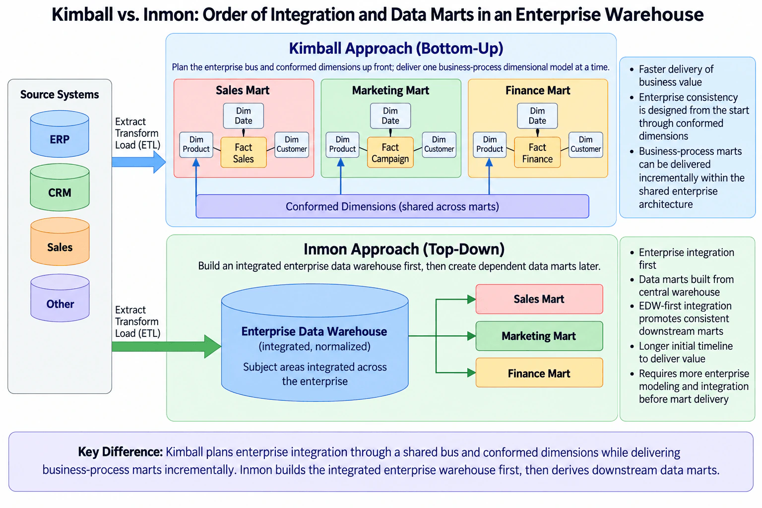
Kimball approach: Plan the enterprise bus and conformed dimensions up front, then implement one business process at a time. The enterprise bus is the architectural plan that shows the important business processes and the dimensions they share. A conformed dimension is a standardized dimension, such as Date, Product, or Customer, whose meaning is reused consistently by multiple fact tables.
In the diagram, Sales, Marketing, and Finance are separate business-process dimensional marts. Each contains a fact table surrounded by dimensions, and the shared conformed dimensions provide consistent descriptive meaning across those marts. Kimball therefore does not mean building unrelated marts and integrating them later. Enterprise consistency is designed from the start, while actual delivery proceeds incrementally.
This incremental delivery is the main practical advantage. A team can release the Sales model, for example, without waiting for every enterprise subject area to be completed. Additional business-process marts can then be added within the same shared architecture. The tradeoff is that conformed dimensions and their definitions must be governed carefully as the environment grows.
Inmon approach: Build the integrated enterprise data warehouse first, then create dependent data marts from it. In the diagram, source data is transformed and loaded into a central enterprise data warehouse that integrates subject areas across the organization. The warehouse is represented as integrated and normalized. Sales, Marketing, and Finance marts are downstream of that warehouse.
Because enterprise integration happens before dependent marts are delivered, the downstream marts start from a common integrated source. This promotes cross-mart consistency. The tradeoff is that more enterprise modeling and integration work normally has to happen before users receive the first marts, so initial delivery can take longer.
The key difference is therefore implementation order. Kimball uses a shared enterprise bus and conformed dimensions while delivering business-process dimensional models incrementally. Inmon establishes the integrated enterprise warehouse first and derives dependent marts afterward.
Technical Approach
Identify where enterprise integration is defined in each architecture.
For Kimball, describe the enterprise bus and conformed dimensions, then explain incremental delivery by business process.
For Inmon, describe the integrated enterprise data warehouse as the central foundation, then explain that dependent marts are created from it.
Compare delivery timing: Kimball can release useful business-process models earlier; Inmon requires more central integration before mart delivery.
Compare cross-mart consistency: Kimball relies on shared conformed dimensions; Inmon relies on downstream marts sourcing from the integrated enterprise warehouse.
Finish with the tradeoff between incremental delivery and integration-first delivery.
Practical Insights
This is an architecture tradeoff, not an algorithm with Big-O complexity. Kimball spreads implementation across business processes, which can reduce the time before the first useful model is delivered. Its ongoing cost is careful management of shared dimensions and definitions as more marts are added. Inmon requires more enterprise modeling and integration before dependent marts are available, increasing upfront effort. Its downstream marts benefit from a common integrated warehouse. Both approaches still require continuing ETL, data-quality, schema, governance, and maintenance work.
Why Interviewers Ask This
Interviewers want to know whether you understand how warehouse architecture affects implementation order, delivery speed, and consistency across analytical areas. A strong answer explains that Kimball combines an enterprise integration blueprint with incremental business-process delivery, while Inmon establishes the integrated enterprise warehouse before dependent marts are produced.
Common interview mistakes
A common mistake is saying that Kimball builds completely independent marts first and only worries about integration later. In the enterprise bus architecture, conformed dimensions provide the integration plan from the start. Another mistake is treating conformed dimensions as outputs of fact tables; they are shared dimensions reused by multiple dimensional models. For Inmon, do not reverse the dependency: the integrated enterprise warehouse is established before the dependent marts. Also avoid claiming that either architecture automatically guarantees perfect consistency, because implementation quality and governance still matter.
Interview tip
Lead with the order of construction. Say that Kimball plans shared conformed dimensions and delivers business-process models incrementally, while Inmon integrates the enterprise warehouse first and derives marts afterward. Then connect that order directly to delivery speed and cross-mart consistency.
Interviewer may ask next
How do conformed dimensions support cross-mart consistency in the Kimball approach?
A conformed dimension uses a standardized meaning and structure across multiple business-process models. For example, Sales, Marketing, and Finance can reuse consistent Date, Product, or Customer dimensions. This lets measures from different fact tables be analyzed together using the same descriptive definitions and is the main mechanism for enterprise integration in the Kimball bus architecture.
What is the main tradeoff of building the enterprise warehouse before data marts in the Inmon approach?
The organization performs more enterprise integration and modeling before dependent marts are delivered, so the first analytical outputs can take longer to reach users. In return, those marts are derived from the same integrated enterprise warehouse, giving them a common central data foundation and promoting consistency across downstream analytical areas.
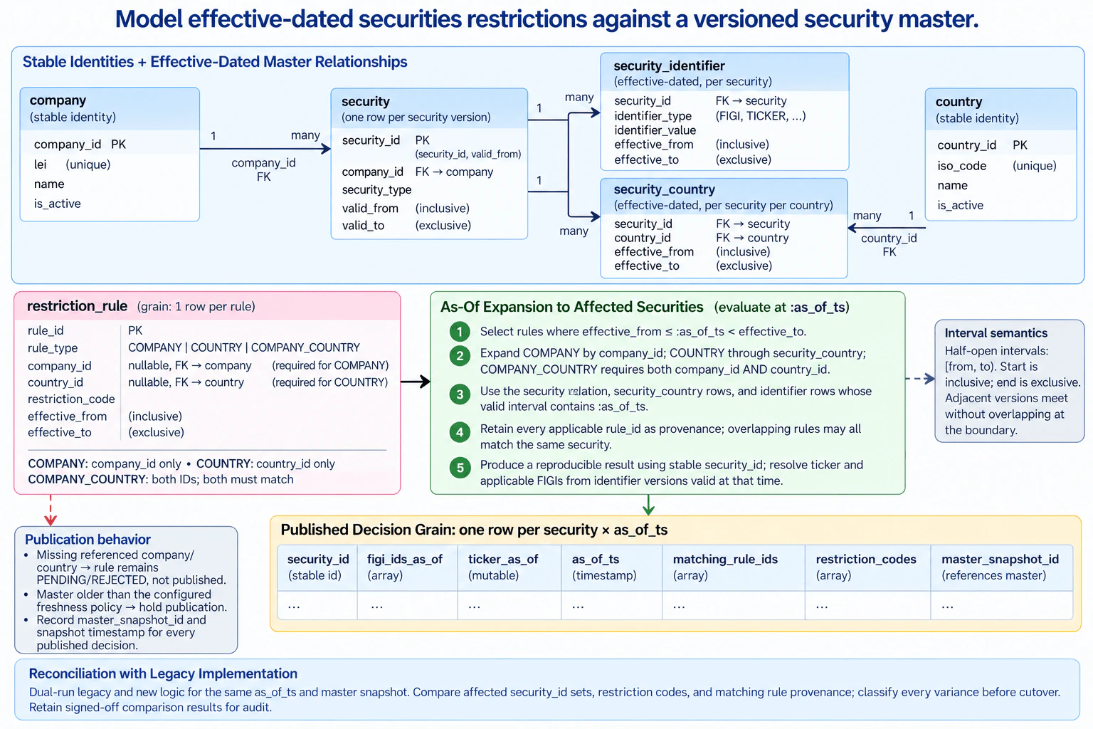
9. Model effective-dated securities restrictions against a versioned security master.Data ModelingMedium
i Question Details
The master relates companies, countries, securities, FIGIs, and mutable tickers. Rules can target a company, a country, or a company-country combination during an effective interval. Define stable identity, versioned relationships, interval boundaries, and exact matching semantics. Explain as-of expansion to affected securities, overlapping-rule provenance, and publication behavior when a referenced company is missing or the master is stale. Preserve reproducible historical decisions through ticker changes and specify reconciliation when replacing a legacy implementation.
Short Interview Answer (30-60 seconds)
Keep company_id, country_id, and security_id stable, but version changing security relationships and identifiers. Evaluate rules and master rows at one as-of timestamp with [from, to) intervals, retain all matching rule IDs, gate publication on a fresh master snapshot, and reconcile legacy results before cutover.
Detailed Explanation
The goal is to decide which securities are restricted at any chosen point in time, even when names, tickers, ownership, or country links change later. We need permanent identities for the important things, a history of what changed and when, and clear start and end times. A rule may apply to one company, one country, or both together. We also need to remember why each security was restricted, avoid publishing from incomplete or old reference information, and be able to reproduce an old decision exactly during audits or migration.
Useful Questions to Ask the Interviewer
Is the as-of value a timestamp or only a business date, and which time zone defines it?
Can a security have more than one applicable FIGI at the same time, and should all applicable FIGIs be returned?
What freshness threshold makes the security master too stale for publication?
Should a rule referencing a missing company or country be rejected permanently, or held pending until the reference arrives?
When multiple restrictions match one security, should consumers receive every restriction code, or is there a separate downstream precedence policy?
What business relationship does security_country represent, such as listing country, trading country, domicile, or another defined association?
How to Explain It in an Interview
Start by separating stable identity from changing relationships. company has stable company_id, country has stable country_id, and a security keeps a stable security_id. The security master is versioned at a grain of one row per security version. A security version contains security_id, company_id, security_type, valid_from, and valid_to; (security_id, valid_from) identifies a version. This lets a security change company relationship over time without changing its permanent security identity.
Identifiers are versioned separately. security_identifier contains security_id, identifier_type, identifier_value, effective_from, and effective_to. This supports mutable tickers and multiple applicable FIGIs while preserving which identifiers were valid historically. security_country is another effective-dated relationship with security_id, country_id, effective_from, and effective_to. A security can therefore have different country relationships over time, while the country itself keeps a stable country_id.
Use one interval convention everywhere: [from, to). The start is inclusive and the end is exclusive. A row is active when from <= as_of_ts AND as_of_ts < to. Half-open intervals let adjacent versions meet exactly at a boundary without both versions being active at that instant.
The restriction_rule table has one row per rule. Its key fields are rule_id, rule_type, nullable company_id, nullable country_id, restriction_code, effective_from, and effective_to. For COMPANY, only company_id is populated. For COUNTRY, only country_id is populated. For COMPANY_COUNTRY, both IDs are populated and both must match. The allowed null patterns should be validated so a missing target value cannot accidentally broaden a rule.
For as-of expansion, first select rules satisfying effective_from <= as_of_ts AND as_of_ts < effective_to. Then resolve the target against master data valid at that same timestamp. A COMPANY rule expands through the valid security version whose company_id matches. A COUNTRY rule expands through valid security_country rows whose country_id matches. A COMPANY_COUNTRY rule requires both the company on the valid security version and the country on a valid security_country row to match.
Every temporal lookup uses the same as_of_ts. That includes the security version, security_country, and security_identifier. This prevents a historical rule from accidentally joining to today's company relationship, ticker, country relationship, or identifier state.
Do not discard overlapping rules merely because several rules affect the same security. Retain every applicable rule_id as provenance. The published decision grain in the model is one row per security_id × as_of_ts, with figi_ids_as_of, ticker_as_of, matching_rule_ids, restriction_codes, and master_snapshot_id. Arrays preserve the multiple FIGIs, matching rules, or restriction codes that can legitimately exist at that grain. If the business later defines precedence or severity, apply that as an explicit downstream policy without losing the original match provenance.
Historical reproducibility comes from the stable security_id, the requested as_of_ts, effective-dated rule and master history, and the exact master_snapshot_id used for publication. A ticker change does not rewrite history because ticker_as_of is resolved from the identifier version valid at the historical timestamp. Applicable FIGIs are resolved from their identifier versions at that same timestamp.
Publication needs a safety gate. If a rule references a company or country missing from the master, keep the rule PENDING or REJECTED and do not publish it as a successful evaluated restriction. If the selected security-master snapshot is older than the configured freshness policy, hold publication. For every published decision, record master_snapshot_id and the snapshot timestamp so the exact reference-data state can be identified later.
When replacing a legacy implementation, dual-run the legacy and new logic using the same as_of_ts and the same master snapshot. Compare affected security_id sets, restriction codes, and matching-rule provenance. Classify every variance, including differences caused by interval boundaries, stale data, missing references, historical ticker handling, company-history handling, or legacy matching logic. Resolve and sign off the differences before cutover, and retain the comparison results for audit.
Technical Approach
Define stable identities for company, country, and security.
Store security company relationships, identifiers, and security-country relationships as effective-dated versions.
Use half-open [from, to) intervals consistently.
Validate the allowed COMPANY, COUNTRY, and COMPANY_COUNTRY target shapes.
At as_of_ts, select active rules.
Resolve the security version, security_country rows, and security_identifier rows valid at the same timestamp.
Expand each active rule to all matching stable security IDs using exact target semantics.
Retain every applicable rule_id and restriction code instead of collapsing overlaps.
Publish one row per security_id × as_of_ts with figi_ids_as_of, ticker_as_of, matching_rule_ids, restriction_codes, and master_snapshot_id.
Hold publication when required references are missing or the master exceeds its freshness policy.
During migration, dual-run old and new logic using identical timestamps and master snapshots and reconcile every variance before cutover.
Practical Complexity & Trade-offs
The main work is finding active rules and then finding the security versions, country relationships, and identifiers that are valid at the requested time. A broad country rule may expand to many securities, so it can cost more than a company-specific rule. Appropriate indexes, clustering, or partitioning can reduce the data read, but the exact physical design depends on the database engine and workload. Keeping historical versions and master-snapshot references uses more storage and needs stronger data-quality checks, but it provides reproducibility and auditability. Maintenance also includes validating rule target shapes, detecting ambiguous master versions, monitoring freshness, and reconciling migration differences.
Where it is used
This model is useful in trading controls, compliance restriction lists, investment-policy enforcement, sanctions or eligibility screening, reference-data-driven risk systems, and any platform that must explain which securities were affected by which rules at a historical point in time. It is especially valuable when tickers, ownership relationships, country associations, or other master-data attributes change while historical decisions must remain reproducible.
Why Interviewers Ask This
This tests whether the candidate can separate stable identity from changing relationships, model temporal relationships correctly, define deterministic interval and matching semantics, preserve provenance when rules overlap, handle stale or incomplete reference data safely, and design a migration that produces reproducible historical decisions rather than silently changing old results.
Common interview mistakes
Common mistakes are using ticker as the stable security identity; overwriting company ownership instead of versioning it; using inclusive end dates and creating ambiguous boundaries; evaluating rules at one timestamp while joining to current master rows; treating nullable company_id or country_id as wildcards instead of validating rule_type semantics; collapsing overlapping rules and losing rule_id provenance; assuming a single FIGI at the published security grain; publishing when a referenced company or country is missing; using stale master data without a publication gate; failing to record the exact master snapshot; allowing multiple ambiguous security versions at one as-of timestamp without handling the data-quality failure; and comparing legacy and replacement systems with different timestamps or snapshots.
Interview tip
Lead with the invariant: stable IDs identify entities, while changing relationships and identifiers are effective-dated. Then state the half-open as-of predicate, explain the three exact rule scopes, retain every matching rule as provenance, and finish with snapshot-based publication and dual-run reconciliation.
Interviewer may ask next
How would you handle two security-master versions that overlap for the same security at the requested as-of timestamp?
Treat that as a master-data quality failure unless simultaneous versions are an explicit part of the model. The intended security-version grain requires one unambiguous version for a security at a point in time. Detect the overlap, hold publication for affected decisions, correct the version history, and retain the failed snapshot information for audit rather than arbitrarily choosing one version.
Why retain every matching rule instead of choosing one winning restriction rule?
Because overlapping rules can independently explain why the same security is restricted. Keeping matching_rule_ids and restriction_codes preserves complete provenance and makes historical decisions auditable. If the business later needs precedence, severity, or one effective action, apply that as a separate documented policy while retaining the full original match set.
10. How would you model currency conversion for financial transactions?Data ModelingMedium
i Question Details
Represent original and reporting currencies, currency-pair exchange rates, and transaction-date conversion so historical reporting does not use today’s rates.
Short Interview Answer (30-60 seconds)
I would keep the original amount and currency on each transaction, store historical rates by currency pair and reporting date, and convert using the rate resolved for the transaction date. I would never overwrite the original value or use today's rate for historical reporting.
The practical decision is to keep what actually happened separate from how we later show it in another currency. Each payment keeps its original amount and money type. A separate list describes the supported money types. Another history stores the value used to change one money type into another for each reporting day. When someone asks for a report, we use the value that belonged to the day of the payment, not the value available today. This means an old report gives the same answer later, even after market values change.
Useful Questions to Ask the Interviewer
Is there one fixed reporting currency, or can the user choose the target currency at report time?
Do we receive one approved rate for every required currency pair and reporting date, or must we derive some pairs?
Should weekends and holidays be pre-resolved to an approved applicable historical rate during ETL?
What decimal precision and rounding policy should be used for converted reporting amounts?
How to Explain It in an Interview
I would model three core tables.
fact_transaction has a grain of one row per financial transaction. Its primary key is transaction_id. It stores transaction_date, the original amount, and currency_code. The currency_code is a foreign key to dim_currency.currency_code. The important rule is that the original amount and original currency are never overwritten by converted values.
dim_currency has a grain of one row per supported currency. Its primary key is currency_code. It also contains descriptive fields such as currency_name and an optional symbol. One currency can be referenced by many transactions. The same currency dimension is reused for the source and target sides of an exchange-rate pair.
dim_exchange_rate has a grain of one row per source currency, target currency, and calendar reporting date. Its composite primary key is (from_currency, to_currency, effective_date). Both from_currency and to_currency are foreign keys to dim_currency.currency_code, and rate is non-null. Each currency can therefore participate in many exchange-rate rows, while one resolved rate row can be used by many transactions that share that pair and reporting date.
The diagram assumes ETL resolves every calendar reporting date to the historical rate considered applicable for that date. This lets the reporting query use the deterministic equality condition r.effective_date = t.transaction_date. If a raw source publishes rates only on business days, ETL must apply the agreed policy for weekends or holidays before reporting. It must not substitute today's rate for an older transaction.
At report time, the query matches fact_transaction.currency_code to dim_exchange_rate.from_currency, matches the requested reporting currency to dim_exchange_rate.to_currency, and matches transaction_date to effective_date. The reporting amount is t.amount * r.rate. The output remains at one row per matched transaction and includes both the original and reporting currencies.
For transactions already in the requested reporting currency, the model stores identity pairs such as USD to USD with rate = 1 for each reporting date. This allows the same join path to retain those transactions without special-case conversion logic.
The diagram's example is transaction 1001 on 2023-05-10. Its original value is 100.00 EUR. The stored EUR to USD rate for that reporting date is 1.10, so 100.00 × 1.10 = 110.00 USD. If the exchange rate changes later, this historical result remains 110.00 USD because the query continues to use the rate resolved for 2023-05-10.
A missing rate is a data-quality failure. Because the illustrated query uses inner joins, a transaction with no matching resolved historical rate would not appear in the result. In production, I would detect missing pair/date rows during ETL or reconciliation and stop or quarantine incomplete reporting rather than silently replacing them with a current rate.
The main tradeoff is that pre-resolving one rate per calendar reporting date creates additional ETL work and rate rows, but it makes reporting simple, deterministic, and reproducible. Keeping original values separate from derived reporting values also protects the source financial fact while allowing reports in different target currencies.
No database product or SQL dialect is named in the question. The SQL below therefore uses dialect-neutral relational syntax and a named bind-value placeholder for the reporting currency. The exact bind-marker syntax should be adapted to the chosen database driver or SQL engine.
Technical Approach
1. Declare fact_transaction at one row per financial transaction and retain its original amount and currency. 2. Maintain dim_currency at one row per supported currency. 3. Maintain dim_exchange_rate at one row per (from_currency, to_currency, effective_date) with a non-null historical rate. 4. During ETL, resolve every required calendar reporting date to its applicable historical rate, including identity pairs such as USD to USD with rate 1. 5. At report time, join the transaction's original currency, requested reporting currency, and transaction date to exactly one resolved rate row. 6. Calculate amount * rate. 7. Return one reporting row per matched transaction while retaining both original and reporting values. 8. Treat a missing historical pair/date rate as a data-quality failure rather than falling back to today's rate.
Practical Complexity & Trade-offs
Storage grows with the number of transactions plus the number of currency-pair and reporting-date combinations retained. Pre-resolving a row for each required reporting date adds ETL work and storage, but it makes report-time lookups simple. Query cost mainly depends on finding the matching rate for the source currency, target currency, and date. Operational maintenance includes loading rates, detecting missing pair/date rows, maintaining identity rates, reconciling historical data, and applying a consistent decimal and rounding policy.
Example
The SQL follows the diagram's one-row-per-transaction reporting flow. It joins each transaction to the resolved historical exchange-rate row using original currency, requested reporting currency, and transaction date. The ETL assumption guarantees at most one rate for the composite pair/date key. Identity rows such as USD to USD with rate 1 let same-currency transactions use the same join. Because these are inner joins, a missing historical rate removes that transaction from this result, so missing rates should be detected and handled as an upstream data-quality failure. The reporting-currency placeholder binds a value, not an identifier.
Code
-- Result grain: one row per transaction that has a resolved historical rate.-- ETL has already resolved one applicable rate per currency pair and reporting date.SELECT
t.transaction_id,
t.transaction_date,
t.amount AS original_amount,
t.currency_code AS original_currency,
rc.currency_code AS reporting_currency,
-- Apply the historical rate for this transaction date; do not use a current rate.
t.amount * r.rate AS amount_in_reporting_currency
FROM
fact_transaction AS t
JOIN dim_exchange_rate AS r
-- Match the transaction's original currency to the source side of the rate pair.ON r.from_currency = t.currency_code
-- Bind the requested reporting currency as a value, never as a dynamic identifier.AND r.to_currency = ?
-- ETL guarantees one resolved rate for this pair and calendar reporting date.AND r.effective_date = t.transaction_date
JOIN dim_currency AS rc
-- Validate and expose the reporting currency represented by the rate row.ON rc.currency_code = r.to_currency;
-- Null/missing-rate behavior: the inner joins intentionally return no row when no-- resolved historical pair/date rate exists; production ETL should detect that as-- a data-quality failure rather than substitute today's rate.-- No transaction boundary is required because this is a read-only reporting query.
Where it is used
This pattern is used in payment platforms, accounting systems, financial data warehouses, expense systems, marketplaces, billing platforms, and multinational reporting. It is useful whenever transactions must remain in their original currencies while analytical, management, or financial reports require a common reporting currency and must reproduce the same historical results later.
Why Interviewers Ask This
This question tests whether the candidate can preserve financial history while defining clear table grains, keys, relationships, date-based rate lookups, numeric conversion logic, and reproducible reporting. It also tests whether the candidate understands why an old transaction must not be recalculated with today's exchange rate and why the original financial value must remain available.
Common interview mistakes
Common mistakes are overwriting the original transaction amount with a converted amount; storing only the latest rate; recalculating historical transactions with today's rate; failing to define the exchange-rate grain and composite key; allowing duplicate rate rows for the same pair and reporting date, which can duplicate transaction output; omitting identity rates for same-currency reporting; silently dropping transactions when a historical rate is missing without monitoring that failure; falling back to a current rate; and ignoring decimal precision or rounding policy.
Interview tip
Lead with the invariant: never overwrite the original financial fact. Then state the grain of all three tables, explain the composite rate key, walk through the transaction-date lookup, and finish by explaining why pre-resolved historical rates make reports reproducible.
Interviewer may ask next
How would you handle weekends or holidays when no new exchange rate is published on the transaction date?
I would resolve that in the rate-loading process, not by using today's rate in the reporting query. ETL would apply the agreed business or accounting rule, such as carrying forward the most recent approved prior rate, and materialize one resolved rate for each required calendar reporting date. The query can then keep the exact equality join on effective_date = transaction_date. The chosen rule should be explicit, auditable, and consistently applied.
What happens if the requested reporting currency is the same as the transaction's original currency?
I would store identity exchange-rate rows, for example USD to USD with rate = 1 for each reporting date. Then those transactions use the same pair/date join as every other conversion. The reporting amount remains equal to the original amount, and no special-case query branch is required.
More questions load as you scroll
Data Engineer Resume Examples
Explore the resume examples below to find the one that best matches your target Data Engineer role.
Disclaimer: This interview guide is for educational and informational purposes only. It is designed to help readers prepare, but it does not guarantee any interview result, hiring decision, offer, or outcome. Interview questions, hiring criteria, and preferred answers can vary by employer, interviewer, industry, location, and time. All answers, examples, and explanations in this guide are suggested examples for interview preparation, not definitive answers or instructions for professional practice. They are based on research and judgment, are provided without warranties of any kind, and should be adapted to the question, role, and applicable laws and professional requirements. Diagrams are simplified illustrations intended to highlight the main concepts and their relationships; actual situations, systems, and practices may be more complex. Alternative approaches may be equally valid or better suited to a particular question, context, or interviewer. To the fullest extent permitted by applicable law, the contributors and publisher are not liable for decisions made, actions taken, or losses incurred based on this guide.
State Laws and Professional Responsibilities: Laws and requirements governing an occupation vary by state and jurisdiction. You are responsible for checking the current laws, licensing requirements, and scope-of-practice rules that apply to your location and role, and for ensuring that your answers and actions comply with them. Adapt examples in this guide to those requirements. This guide is not legal advice.
Content Accuracy and Verification: To the fullest extent permitted by applicable law, we do not represent or warrant that interview guides, questions, answers, examples, or diagrams are accurate, complete, current, error-free, or suitable for any particular purpose. You are responsible for independently reviewing and verifying the information before relying on it.