This interview guide is for educational and informational purposes only. It is designed to help readers prepare, but it does not guarantee any interview result, hiring decision, offer, or outcome. Interview questions, hiring criteria, and preferred answers can vary by employer, interviewer, industry, location, and time. All answers, examples, and explanations in this guide are suggested examples for interview preparation, not definitive answers or instructions for professional practice. They are based on research and judgment, are provided without warranties of any kind, and should be adapted to the question, role, and applicable laws and professional requirements. Diagrams are simplified illustrations intended to highlight the main concepts and their relationships; actual situations, systems, and practices may be more complex. Alternative approaches may be equally valid or better suited to a particular question, context, or interviewer. To the fullest extent permitted by applicable law, the contributors and publisher are not liable for decisions made, actions taken, or losses incurred based on this guide.
State Laws and Professional Responsibilities
Laws and requirements governing an occupation vary by state and jurisdiction. You are responsible for checking the current laws, licensing requirements, and scope-of-practice rules that apply to your location and role, and for ensuring that your answers and actions comply with them. Adapt examples in this guide to those requirements. This guide is not legal advice.
Identity, Image, and Privacy Notice
To respect individual privacy, some names, profile photographs, avatars, biographical details, and other identifying information displayed in this guide may be replaced with pseudonyms, licensed stock images, illustrative avatars, composite images, or representative descriptions. Unless a person is expressly identified as an actual contributor, a displayed name, image, or profile should not be understood as depicting or identifying a specific candidate, interviewer, employee, or other real individual. These representations are provided for editorial and illustrative purposes only and do not imply endorsement, employment, participation, or affiliation with this guide or any company mentioned in it. Any resemblance to an actual person is coincidental.
Company Notice
This guide is an independent educational resource and is not affiliated with, endorsed by, sponsored by, or approved by the company named in this guide. Company names identify reported interview experiences or the employer context of clearly labeled original practice exercises. Interview practices can change without notice, and inclusion of company-specific content does not mean these questions are official, complete, or guaranteed to be asked. To the fullest extent permitted by law, the author, contributors, and publisher are not responsible for outcomes related to use of this material.
Content Accuracy and Verification
To the fullest extent permitted by applicable law, we do not represent or warrant that interview guides, questions, answers, examples, or diagrams are accurate, complete, current, error-free, or suitable for any particular purpose. You are responsible for independently reviewing and verifying the information before relying on it.
Questions or comments?
Contact us for general questions, or share feedback, technical corrections, and comments with the community.
21. Compare Airflow’s poke, reschedule, and deferrable waiting mechanisms.Data PipelinesMedium
i Question Details
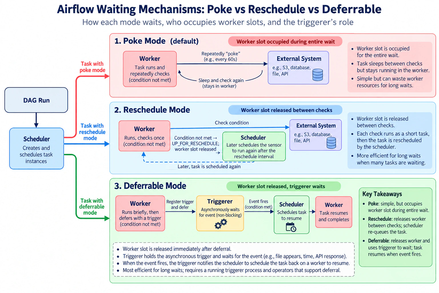
Explain worker-slot occupancy and the triggerer’s role during a wait.
Short Interview Answer (30-60 seconds)
The big difference is what happens to the worker while a task waits. Poke keeps a worker slot occupied and repeatedly checks the external condition. Reschedule checks once, releases the worker, and lets the scheduler run the sensor again later. Deferrable execution releases the worker and moves the wait to an asynchronous trigger in the triggerer. When the trigger fires, the scheduler queues the task to resume on a worker. For long waits, deferrable execution usually uses worker capacity most efficiently.
Detailed Explanation
The question is asking how three ways of waiting use shared computing capacity. Imagine a job must pause until a file, database result, API response, or another outside condition is ready. One choice keeps a machine busy while checking again and again. Another gives that machine back and tries again later. The third gives the machine back and uses a lightweight watcher for the waiting period. The important comparison is who waits, when the main worker is released, and how the job gets scheduled to continue.
Useful Questions to Ask the Interviewer
Are we comparing a sensor that supports all three waiting approaches, or should I explain the mechanisms conceptually?
Is the expected wait usually short and frequent, or long enough that worker capacity is a major concern?
How to Explain It in an Interview
1. Start with worker-slot occupancy
I would start with the main decision: whether a waiting task should continue occupying a worker slot. A worker slot is execution capacity that could run another task. In the diagram, all three paths are managed by Airflow, but they use that capacity differently. Poke keeps the worker for the full wait. Reschedule releases it between checks. Deferrable execution also releases it, but moves the waiting logic to the triggerer.
2. Poke mode keeps the worker occupied
In poke mode, the sensor runs on a worker and checks the External System, such as S3, a database, a file, or an API. If the condition is not ready, the sensor sleeps and checks again after its poke interval. The important point is that the task stays on the worker for the entire wait. This is simple and can work well for short waits or frequent checks, but many long-running poke sensors can consume worker slots while mostly idle.
3. Reschedule mode releases the worker between checks
In reschedule mode, the worker runs the sensor long enough to check the External System once. If the condition is not met, the task enters its rescheduling wait, shown in the diagram as UP_FOR_RESCHEDULE, and the worker slot is released. The scheduler later schedules the sensor to run again after the reschedule interval. The next check uses a worker again, but only for that execution. This is more worker-efficient than poke for longer waits with periodic polling. The trade-off is repeated scheduler-driven execution.
4. Deferrable execution moves the wait to the triggerer
With deferrable execution, the worker starts the task and the operator defers when it reaches the waiting point. A trigger is registered and the worker is released. The triggerer is a separate Airflow component that runs lightweight asynchronous triggers. In the diagram, the triggerer owns the waiting period instead of a normal worker. When the trigger fires because the condition is met, the scheduler queues the task to resume on a worker. The worker then continues and completes the task.
5. Choose based on the waiting pattern
I would use poke when the wait is short or frequent polling is important and holding a worker is acceptable. I would use reschedule when a sensor should perform simple checks at intervals without occupying a worker between those checks. I would prefer deferrable execution for long or event-oriented waits when the operator or sensor supports deferral and the Airflow deployment has a running triggerer. Its main advantage is that many waiting tasks can share the triggerer's asynchronous execution rather than consuming many worker slots.
6. Keep component responsibilities separate
The worker executes the sensor or operator code. The External System only exposes the condition being checked; it does not schedule Airflow tasks. In reschedule mode, the scheduler arranges the later execution after the reschedule interval. In deferrable mode, the triggerer owns the asynchronous wait, and the scheduler queues the task to resume after the trigger fires. Keeping those responsibilities separate is the main control-flow correctness point.
Technical Approach
Identify how long the task may wait and how frequently the condition must be checked.
Decide whether holding a worker slot during that wait is acceptable.
Use poke for short or frequent polling when continuous worker occupancy is acceptable.
Use reschedule for periodic checks that should release the worker between executions.
Use deferrable execution when the operator supports it, a triggerer is running, and long or event-driven waits should avoid worker occupancy.
Trace the resume path correctly: the triggerer owns the asynchronous wait, while the scheduler arranges later worker execution.
Practical Insights
The benefit of poke is simplicity and potentially low response delay because the same task stays active and checks repeatedly. The downside is worker capacity: every waiting sensor keeps occupying a worker slot. Reschedule reduces that cost because the worker is used only for each check, but repeated checks create more scheduler activity. Deferrable execution is usually the most efficient for long waits because many asynchronous triggers can share the triggerer instead of holding normal workers. The downside is an extra operational dependency: a triggerer must be running, and the operator or sensor must support deferral. We accept that extra dependency when freeing worker capacity during long waits is more valuable than keeping the waiting logic on workers.
Why Interviewers Ask This
Interviewers ask this to test whether you understand that waiting is also a resource-management decision. A strong answer separates worker execution, scheduler control, and asynchronous trigger execution. It shows that you can choose between continuous polling, periodic rescheduling, and deferral based on wait duration and operator support. They also want to see whether you can trace task state correctly and explain which Airflow component owns each part of the wait and resume flow.
Common interview mistakes
Common mistakes are saying that reschedule keeps the worker occupied, saying that the External System schedules the next sensor run, or treating the triggerer as another normal worker. Another mistake is claiming that deferrable execution eliminates the scheduler; it does not. The triggerer handles the asynchronous wait, but the scheduler still queues the task to resume on a worker. Candidates also sometimes describe reschedule and deferrable as identical because both release the worker. The key difference is who owns the waiting period: repeated scheduler-driven executions for reschedule versus an asynchronous trigger in the triggerer for deferrable execution.
Interview tip
Lead with worker-slot occupancy, then compare the three modes in order: poke holds the worker, reschedule releases it between scheduled checks, and deferrable releases it while the triggerer waits asynchronously. Finish by explaining the resume path and when you would choose each option.
Interviewer may ask next
What would you change if thousands of Airflow tasks needed to wait for external events at the same time?
I would prefer deferrable operators or sensors when those tasks support deferral and the Airflow deployment has a running triggerer. The changed requirement is concurrency: thousands of mostly idle waits make worker-slot efficiency much more important. With poke mode, each waiting task can hold worker capacity, so enough waiting sensors can prevent active work from running. Reschedule avoids holding workers between checks, but thousands of periodically rescheduled sensors still create repeated scheduler activity. With deferrable execution, each worker runs only until the task defers. The triggerer then runs the lightweight asynchronous triggers while workers remain available for active tasks. When a trigger fires, the scheduler queues that task to resume on a worker. The External System and the rest of the DAG remain unchanged. Correctness stays intact because the trigger only determines when the task may resume; the worker still executes the task logic. The main downside is depending on sufficient triggerer capacity and on operators that correctly support deferral.
How would you choose between reschedule and deferrable mode for a long wait?
I would choose based on how the wait is detected and what the operator supports. If the condition is naturally checked at fixed intervals and the sensor supports reschedule mode, reschedule is reasonable. The worker checks the External System once, releases its slot when the condition is not met, and the scheduler arranges another execution after the reschedule interval. If the operator supports deferral and the deployment has a triggerer, I would usually prefer deferrable execution for a long or event-oriented wait. The worker defers, the triggerer owns the asynchronous wait, and the scheduler sends the task back to a worker after the trigger fires. In both designs, the External System does not schedule the Airflow task, and normal worker capacity remains free while waiting. The main downside of reschedule is repeated scheduler-driven execution. The main downside of deferrable execution is the triggerer dependency and the requirement that the operator or sensor support deferral.
22. Design a pipeline that identifies unhealthy pods by comparison with sibling replicas.Data PipelinesMedium
i Question Details
The input is disorganized historical pod alerts; the pipeline must turn that history into structured comparison signals.
Short Interview Answer (30-60 seconds)
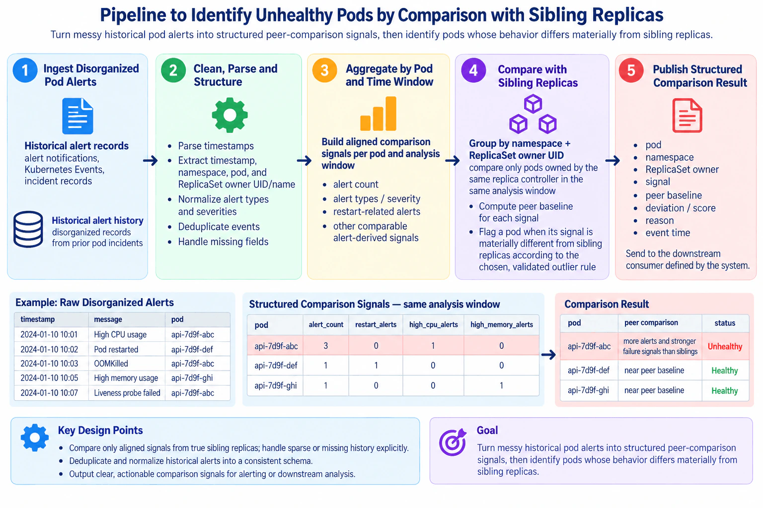
I would normalize the historical pod alerts, extract pod, namespace, timestamp, and ReplicaSet owner identity, then aggregate comparable alert-derived signals for each pod over the same analysis window. Pods are grouped by namespace and ReplicaSet owner UID so only true siblings are compared. I would compute a peer baseline and use a validated outlier rule to flag material differences. The main trade-off is sensitivity versus false positives, especially when a replica group has sparse history.
Detailed Explanation
This question asks us to turn a messy history of pod alerts into a fair way to find one pod that behaves differently from the other copies doing the same job. First, the old alert records are cleaned and organized. Next, each pod is placed into the correct sibling group and its alerts are summarized over the same period. Those summaries are compared with the other replicas. The result should say which pod looks unhealthy, what was different, and when it happened, without comparing unrelated pods or relying on an arbitrary limit.
Useful Questions to Ask the Interviewer
Do the historical records contain timestamp, pod, namespace, and ReplicaSet owner UID or name, or must any of those fields be reconstructed from existing alert metadata?
How should the common analysis window be chosen for all sibling pods?
Which alert-derived signals should be considered meaningful for the comparison?
How should the pipeline behave when a pod or sibling group has sparse or missing history?
Should the output contain only healthy or unhealthy status, or also the peer baseline, deviation or score, and explanation?
How to Explain It in an Interview
1. Clean, parse, and structure the historical alerts
I would start with the historical alert records because they are the source shown in the design. For each record, I would parse the timestamp and extract the pod, namespace, and ReplicaSet owner UID or name. I would normalize alert types and severities so equivalent alerts have a consistent representation. I would also deduplicate repeated events and keep missing fields explicit rather than silently turning them into zeros. The result of this stage is a consistent record shape that can be grouped and compared reliably.
2. Build aligned comparison signals per pod
Next, I would aggregate the normalized records by pod for the same analysis window. The diagram uses alert-derived signals such as alert count, alert type or severity, restart-related alerts, and other comparable signals found in the history. The critical rule is alignment: sibling replicas must be evaluated over the same period and from comparable data. Missing history is not the same as healthy behavior, so sparse or missing evidence should remain visible to the comparison logic.
The worked example illustrates this transformation. Pod api-7d9f-abc has three historical alerts: High CPU usage, OOMKilled, and Liveness probe failed. Pod api-7d9f-def has one Pod restarted alert. Pod api-7d9f-ghi has one High memory usage alert. The structured table therefore records alert counts of 3, 1, and 1 respectively, with the matching restart, high-CPU, and high-memory alert indicators.
3. Group only true sibling replicas
Before calculating a peer baseline, I would group pods by namespace and ReplicaSet owner UID. That is the sibling boundary in the diagram. Pods that merely have similar names should not be compared if they belong to different ReplicaSet owners. Within each valid sibling group, I would use only records from the same analysis window. This grouping decision is important because a good anomaly calculation is still wrong if the peer set contains unrelated workloads.
4. Compare each pod with the sibling baseline
For every comparison signal, I would compute a peer baseline from the sibling replicas and measure how much each pod differs from that baseline. I would not hard-code an arbitrary numeric threshold because the diagram deliberately leaves the outlier rule open. Instead, the rule should be chosen and validated against the available history, expected noise, and replica-group size. In the worked example, api-7d9f-abc has more total alerts and additional failure-type alerts than its siblings, so the comparison marks it unhealthy while api-7d9f-def and api-7d9f-ghi remain near the peer baseline.
5. Publish the structured comparison result
The final stage publishes a structured comparison result. The fields shown are pod, namespace, ReplicaSet owner, signal, peer baseline, deviation or score, reason, and event time. The reason matters because downstream users should be able to understand why a pod was flagged rather than seeing only a binary label. The exact downstream consumer is intentionally unspecified because the question and diagram do not choose one.
6. Protect comparison quality
The main correctness risks are duplicate alerts, missing fields, sparse history, incorrect sibling grouping, and misaligned analysis windows. Deduplication prevents one repeated alert from unfairly increasing a pod's signal. Explicit handling of missing history prevents absence of data from looking like healthy behavior. Namespace plus ReplicaSet owner UID prevents unrelated pods from entering the baseline. Finally, the outlier rule must be validated instead of using an unsupported fixed threshold. The trade-off is sensitivity versus false positives: an aggressive rule reacts sooner but may create noise, while a conservative rule needs stronger evidence before marking a pod unhealthy.
Technical Approach
Read the disorganized historical pod alert records.
Parse timestamps and extract pod, namespace, and ReplicaSet owner UID or name.
Normalize alert types and severities, deduplicate repeated alerts, and keep missing fields explicit.
Aggregate comparable alert-derived signals per pod for one common analysis window.
Group pods by namespace and ReplicaSet owner UID so only true sibling replicas are compared.
Compute a peer baseline for each signal inside each sibling group.
Apply a chosen, validated outlier rule to identify materially different pod behavior.
Publish the structured comparison result with pod, namespace, ReplicaSet owner, signal, peer baseline, deviation or score, reason, and event time.
Practical Insights
The main processing cost comes from cleaning every historical alert, grouping records by pod and sibling set, and calculating peer baselines. If there are N alert records, normalization and aggregation grow roughly with N, plus the work needed to compare pods inside each ReplicaSet group. Memory depends mainly on how much history is held for the active analysis window. The benefit is that each pod is judged against relevant siblings instead of one global threshold. The downside is that small replica groups or sparse history can produce weak baselines. A more sensitive outlier rule can detect unusual behavior sooner, but it can also create more false positives. We accept this trade-off because the rule can be validated against historical behavior rather than chosen arbitrarily.
Why Interviewers Ask This
This question tests whether a candidate can turn messy operational history into a trustworthy comparison signal. The interviewer is looking for judgment about data contracts, correct sibling grouping, aligned analysis windows, duplicate and missing records, peer-based anomaly detection, and explainable outputs. It also tests whether the candidate avoids inventing technologies or arbitrary thresholds and can separate reliable data preparation from the final health decision.
Common interview mistakes
Common mistakes are comparing pods from different ReplicaSets, grouping by similar pod names instead of namespace plus ReplicaSet owner identity, comparing different time windows, counting duplicate alerts as separate evidence, and interpreting missing history as zero activity. Another mistake is inventing a fixed outlier threshold without validating it. Candidates may also produce only a healthy or unhealthy label and omit the peer baseline, deviation or score, reason, and event time that make the result explainable.
Interview tip
Lead with the core comparison rule: normalize the alert history, identify true siblings with namespace plus ReplicaSet owner UID, build aligned per-pod signals, and compare each pod with its peer baseline. Mention deduplication and sparse history early. Do not introduce a vendor, storage system, scheduler, or numeric threshold that the question does not specify.
Interviewer may ask next
What would you change if the unhealthy-pod signal had to update much sooner as new alerts arrive?
I would keep the same logical pipeline and shorten the time between evaluations rather than replace the design. The freshness requirement changes, but the contracts remain the same: each new alert still needs a timestamp, pod, namespace, normalized alert type or severity, and ReplicaSet owner identity. The aggregation stage would update per-pod signals for a smaller current analysis window, and the comparison stage would recompute the peer baseline for the corresponding sibling group. Correctness still depends on comparing replicas over aligned windows and not treating missing or delayed history as healthy evidence. If an evaluation cannot build a trustworthy peer set, it should avoid producing an overconfident health decision. The published record keeps the same fields: pod, namespace, ReplicaSet owner, signal, peer baseline, deviation or score, reason, and event time. The main downside is that shorter windows contain less evidence, so results may become noisier and the validated outlier rule may need more conservative behavior.
How would you handle a ReplicaSet where one or more sibling pods have very little historical alert data?
I would treat sparse history as insufficient evidence, not as healthy behavior. The affected parts are the aggregation and peer-comparison stages; the rest of the pipeline stays the same. Historical records should still be normalized and deduplicated, and pods should still be grouped only by namespace and ReplicaSet owner UID. During aggregation, the pipeline should keep the fact that some pods have little or missing history visible instead of replacing missing observations with invented zeros. The comparison logic should then use only aligned, comparable evidence and avoid making a strong outlier decision when the peer baseline is too weak. The published reason can state that evidence is limited when a confident comparison is not possible. Once additional historical records become available, the same signals and baseline can be recomputed using the original design. The downside is fewer decisive classifications, but that is safer than generating false confidence from an incomplete sibling baseline.
23. When would Snowflake Dynamic Tables be appropriate for transformation pipelines?Data PipelinesMedium
i Question Details
Discuss declarative query definitions, target lag, and managed refresh responsibilities.
Short Interview Answer (30-60 seconds)
I would use Snowflake Dynamic Tables when the data is already in Snowflake and the transformation can be expressed in SQL. I can define Bronze, Silver, and Gold results declaratively, set a target lag for desired freshness, and let Snowflake manage refresh scheduling and dependencies. The trade-off is simpler operations versus less exact control over refresh timing, with tighter freshness potentially using more compute.
Detailed Explanation
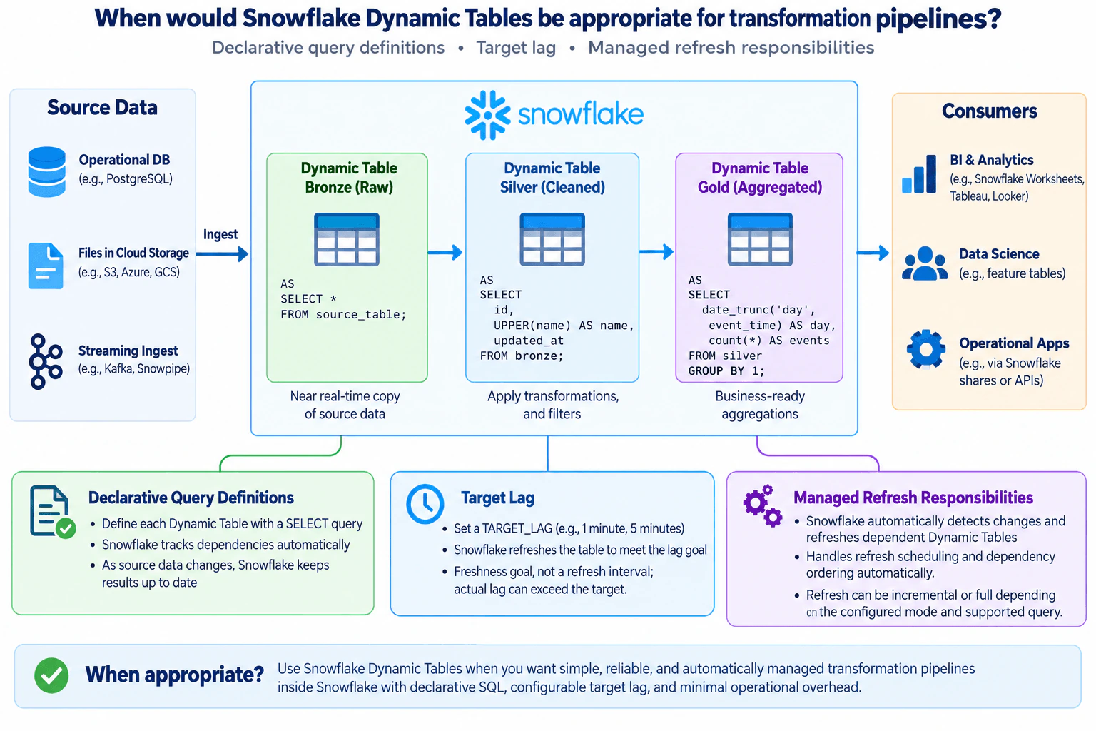
This question asks when it is useful to let Snowflake keep transformed data current instead of operating separate scheduled transformation jobs. The main idea is simple: describe what each result should look like, choose how fresh it should be, and let Snowflake manage when those results are refreshed. In the diagram, data comes from operational systems, cloud files, or streaming ingestion, becomes available in Snowflake, then passes through raw, cleaned, and summarized layers before serving reporting, data science, and applications. The decision is mainly about simplicity, freshness, compute cost, and how much scheduling control you need.
Useful Questions to Ask the Interviewer
Is the source data already available inside Snowflake before these transformations begin?
How fresh do the Bronze, Silver, and Gold results need to be?
Is a freshness goal enough, or does the workflow require an exact execution schedule?
Are the transformation queries compatible with the desired Dynamic Table refresh mode?
How to Explain It in an Interview
1. Separate ingestion from the Dynamic Table pipeline
I would first separate source ingestion from transformation. The diagram shows an Operational DB, Files in Cloud Storage, and Streaming Ingest at the source boundary. Those paths make data available to Snowflake; the Dynamic Tables then operate on data that is already accessible inside Snowflake.
The Bronze Dynamic Table represents the first maintained transformation layer. The diagram shows it as SELECT * FROM source_table, creating a raw or near-raw result. The important point is that Dynamic Tables do not replace the external ingestion mechanisms shown on the left. They maintain downstream query results once the required source data is available in Snowflake.
2. Define the transformation graph declaratively
I would then define each transformation by describing the desired SQL result. The diagram moves from Dynamic Table Bronze (Raw) to Dynamic Table Silver (Cleaned), then to Dynamic Table Gold (Aggregated).
Silver derives cleaned fields from Bronze. Gold reads Silver and produces a daily aggregation with date_trunc('day', event_time) and count(*). These SQL definitions create a dependency chain. Snowflake tracks those dependencies automatically, so the candidate focuses on what each table should contain rather than writing a separate scheduler for every dependency.
This is a strong fit when the transformation logic is naturally expressed as SQL and the derived results should stay current automatically.
3. Treat TARGET_LAG as a freshness goal
Target lag is the main freshness control in this design. I would explain it as the desired maximum staleness of a Dynamic Table relative to its upstream data, not as a fixed instruction to run every N minutes.
The diagram shows examples such as one minute or five minutes. Snowflake schedules refresh work to try to satisfy that lag goal. Actual lag can exceed the target, so I would never present it as a hard timing guarantee.
A shorter target lag asks for fresher data and can require more refresh work and compute. A longer lag is appropriate when consumers can tolerate older results and lower refresh pressure is more important.
4. Let Snowflake own refresh scheduling and dependency ordering
The major operational advantage is that Snowflake manages the refresh process shown in the diagram. It detects relevant upstream changes, schedules refreshes, and respects dependencies between the Bronze, Silver, and Gold Dynamic Tables.
The refresh itself can be incremental or full depending on the configured refresh mode and whether the query supports that mode. I would not claim that all Dynamic Tables always refresh incrementally.
This removes much of the custom orchestration needed for this SQL transformation chain. It does not mean the candidate controls an exact cron-like execution time for every table; the design is driven by freshness goals instead.
5. Serve the maintained Gold result to consumers
The final Gold Dynamic Table contains the business-ready aggregation. The diagram sends that result to BI & Analytics, Data Science, and Operational Apps. It can also serve as an upstream result for downstream tables.
This makes Dynamic Tables a good fit when those consumers need automatically maintained data inside Snowflake and can work with a freshness objective instead of exact user-controlled execution times. The data path remains Bronze to Silver to Gold, and Snowflake maintains that dependency chain.
6. Choose Dynamic Tables when managed simplicity matches the requirement
The benefit is simpler operation. The engineer maintains declarative SQL and freshness targets instead of a collection of separately scheduled transformation jobs. The downside is reduced control over exact refresh timing, and aggressive freshness goals can increase compute consumption.
I would therefore choose Dynamic Tables for Snowflake-centered, SQL-based transformation pipelines where managed dependencies and target-lag freshness are desirable. I would be less likely to choose them when the workflow depends on exact external scheduling or processing behavior that does not fit the supported Dynamic Table refresh model.
Technical Approach
Confirm that the required source data is available inside Snowflake after the ingestion boundary.
Define Dynamic Table Bronze (Raw) from the Snowflake source table.
Define Dynamic Table Silver (Cleaned) from Bronze for the required transformations.
Define Dynamic Table Gold (Aggregated) from Silver for the business-ready aggregation.
Set TARGET_LAG according to the freshness requirement.
Let Snowflake manage refresh scheduling and dependency ordering across the Dynamic Tables.
Use an incremental or full refresh mode according to configuration and query support.
Serve the Gold result to BI & Analytics, Data Science, downstream tables, or Operational Apps.
Verify that observed freshness and compute usage remain acceptable.
Practical Insights
The benefit is lower operational complexity because Snowflake manages refresh scheduling and dependency ordering for this SQL transformation chain. The engineer mainly maintains query definitions and freshness goals instead of separate scheduled jobs. The downside is that target lag is a freshness goal, not an exact schedule or hard guarantee. A shorter lag can make data fresher but may require more compute. A longer lag can reduce refresh pressure but gives consumers older data. Incremental refresh can reduce the amount of recomputation when it is supported, while full refresh can require more work. We accept these trade-offs when simpler managed transformations are more valuable than precise control over each execution time.
Why Interviewers Ask This
Interviewers ask this to test whether you can choose a managed transformation feature for the right workload instead of building custom scheduled jobs by default. They want to see whether you understand declarative SQL transformations, target-lag freshness, dependency management, managed refresh behavior, and compute trade-offs. A strong answer also separates external ingestion from transformation inside Snowflake and does not mistake target lag for a fixed refresh interval.
Common interview mistakes
A common mistake is saying TARGET_LAG means the Dynamic Table executes on a fixed interval. It is a freshness goal, and actual lag can exceed the target. Another mistake is assuming every refresh is incremental; refreshes can be incremental or full depending on the configured mode and query support. Candidates also sometimes blur ingestion and transformation by implying that the Dynamic Tables themselves directly ingest the Operational DB, cloud files, or streaming source. In this diagram, ingestion is a separate boundary before the Snowflake transformation chain. Another mistake is promising very low freshness without considering compute cost. Finally, Dynamic Tables should not be described as a replacement for every orchestrator; they are strongest when the transformation graph fits Snowflake's SQL and managed-refresh model.
Interview tip
Lead with the decision: use Dynamic Tables when data is already in Snowflake, transformations are SQL-based, and you want declarative definitions, target-lag freshness, and Snowflake-managed dependencies. Then clarify that target lag is a freshness objective rather than a cron schedule. Finish with the main trade-off: simpler orchestration and maintenance in exchange for less exact refresh-time control and potentially more compute for tighter freshness.
Interviewer may ask next
What would you change if the Gold Dynamic Table suddenly needed much fresher data?
I would first reduce the target lag only if the business requirement truly needs fresher Gold data. That changes the freshness requirement, not the Bronze-to-Silver-to-Gold architecture. Snowflake would still manage refresh scheduling and dependency ordering across the same Dynamic Tables.
Next, I would check whether the Bronze, Silver, and Gold transformations can keep up with the tighter goal and whether their configured refresh modes are appropriate. I would not claim that lowering target lag creates an exact execution interval or guarantees the table will always remain within that lag. Actual lag can still exceed the target.
The SQL definitions and consumer flow stay the same. No new retry, replay, or custom recovery path is shown in this design, so I would not invent one. I would validate the change by checking the observed freshness of the Gold result after refreshes.
The main downside is compute cost. A tighter freshness goal can cause more refresh work. If consumers do not truly need that freshness, retaining a longer lag is usually more economical.
What if the Silver transformation cannot use incremental refresh?
I would keep the same Dynamic Table pipeline and use refresh behavior that the Silver query and configuration support. The affected component is Dynamic Table Silver (Cleaned); the logical Bronze-to-Silver-to-Gold flow does not need to change just because incremental refresh is unavailable.
If Silver must use full refresh behavior, Snowflake can still manage its refresh scheduling and dependency ordering with Gold. The SQL result contract should remain the same so downstream consumers continue receiving the expected cleaned and aggregated data.
No separate failure-recovery mechanism is shown in the diagram, so I would not add an invented retry or backfill workflow. I would validate the change by checking that Silver and Gold still reach acceptable freshness and produce the expected results after refreshes.
The main downside is additional work and compute. A full refresh can recompute more data than an incremental refresh. If that cost or duration becomes unacceptable, I would reconsider the Silver query design only if the required business result can remain unchanged.
24. How is runtime task mapping different from dynamically generating Airflow DAGs?Data PipelinesHard
i Question Details
Contrast execution-time inputs with parse-time topology, including mapped-instance limits and concurrency controls.
Short Interview Answer (30-60 seconds)
The big difference is when the shape is decided. Dynamic DAG generation creates DAGs or tasks while Airflow parses the DAG file, so topology comes from code or configuration already available then. Runtime task mapping keeps one mapped task in that parsed topology and expands it into task instances when runtime data arrives. Mapping is better for data-driven fan-out. The trade-off is runtime orchestration load, so max_map_length bounds the mapping size and max_active_tis_per_dag controls concurrent mapped execution.
Detailed Explanation
This question asks when a workflow should decide how much repeated work exists. One approach decides the structure before a run starts, using information already available when the workflow definition is read. The other keeps one placeholder for repeated work and waits until a run produces its list of items. It then creates one piece of work for each item. The key decision is whether the amount of work is known beforehand or discovered during execution, and how to prevent a very large runtime list from creating too many task instances at once.
Useful Questions to Ask the Interviewer
Is the number of tasks known from configuration before the DAG is parsed, or is it discovered from an upstream task during each run?
Should each configuration create a separate DAG, or should one DAG fan out over runtime items?
What maximum mapped-task fan-out and concurrency should the workflow allow?
How to Explain It in an Interview
1. Separate parse time from execution time
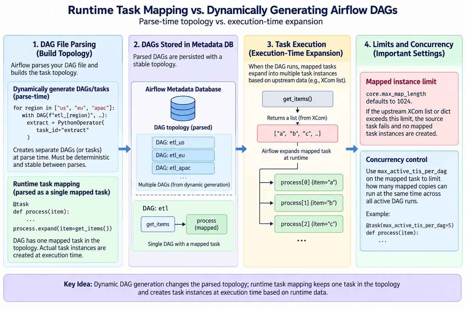
I would first separate DAG construction from DAG execution. When Airflow processes the DAG file, it builds the workflow topology. In the diagram, the parse-time example loops over regions such as us, eu, and apac and creates etl_us, etl_eu, and etl_apac. That is dynamic DAG generation: code or configuration available during parsing determines which DAGs or tasks exist. The generated structure should be deterministic and stable between parses so Airflow presents a predictable topology.
2. Dynamic generation changes the parsed topology
After parsing, the diagram shows the generated DAG topology in the Airflow metadata layer. The region example results in multiple DAGs. The important point is that this structure is determined before a particular DAG run receives runtime task output. Dynamic DAG generation therefore fits configuration-driven topology. It is not the right mechanism when the task count depends on a value that an upstream task discovers only during execution.
3. Runtime mapping keeps one mapped task in the topology
For runtime mapping, the parsed DAG contains an upstream task such as get_items and one mapped process task. The parse-time topology does not need separate process[0], process[1], and process[2] task definitions. When the DAG runs, get_items() produces runtime data, represented in the diagram as a list such as ["a", "b", "c", ...]. That result becomes the input used to expand the mapped task.
4. Expansion happens during the DAG run
Airflow uses the runtime collection to determine how many mapped task instances are needed. If the collection contains three items, the mapped task can produce instances such as process[0], process[1], and process[2], with each instance receiving one corresponding item. This is why Dynamic Task Mapping is the appropriate choice for data-driven fan-out: different DAG runs can discover different numbers of items while keeping the same basic parsed dependency graph.
5. Bound the mapping size
Runtime fan-out needs a safety limit. The diagram shows core.max_map_length, which defaults to 1024. If an XCom value used for mapping contains more items than this configured limit allows, the task that pushed that value fails rather than allowing an excessively large mapping expansion. This is a fan-out size guard. It does not mean that all allowed mapped task instances may execute simultaneously.
6. Bound concurrent mapped execution
The separate concurrency control is max_active_tis_per_dag on the mapped task. It limits how many instances of that task can run concurrently across active DAG runs. For example, setting it to 5 can allow a larger mapped collection to exist while only a bounded number of process instances run at once. The benefit is controlled scheduler and worker pressure. The downside is that lower concurrency can increase the total completion time.
7. Choose based on when the information exists
My decision rule is simple: if code or configuration already knows the required DAG or task structure at parse time, dynamic DAG generation is appropriate. If an upstream task discovers the collection during execution, use Dynamic Task Mapping. Dynamic generation gives predictable configuration-driven topology. Mapping gives flexible runtime fan-out, but the mapping size and concurrent execution need explicit operational limits.
Technical Approach
Determine when the information that controls task count becomes available.
If code or configuration knows it while the DAG file is parsed, generate the required DAGs or tasks deterministically at parse time.
If an upstream task produces the collection during the DAG run, keep one mapped task in the parsed topology and expand it from that runtime result.
Check core.max_map_length so unexpectedly large mapping input cannot create uncontrolled fan-out.
Use max_active_tis_per_dag when the mapped task needs bounded concurrent execution across active DAG runs.
Verify that the selected mechanism matches the intended parse-time or execution-time boundary.
Practical Insights
The benefit is that each approach puts complexity in the right place. Dynamic DAG generation makes runtime behavior predictable because the topology is already known, but generating many DAGs or tasks can increase parsing and metadata work. Runtime mapping keeps the DAG definition compact and adapts to data discovered during a run. The downside is that a large runtime collection can create many task instances and increase scheduler, metadata, and worker pressure. max_map_length bounds the mapping input size, while max_active_tis_per_dag bounds concurrent instances of the mapped task across active DAG runs. We accept the extra runtime coordination because mapping is the correct choice when fan-out cannot be known during parsing.
Why Interviewers Ask This
Interviewers ask this to test whether a candidate understands the boundary between DAG definition and DAG execution. A strong answer distinguishes parse-time topology from runtime fan-out, chooses the correct mechanism based on when the required information becomes available, and understands the operational controls around mapped tasks. It also shows judgment about scheduler and metadata pressure, bounded concurrency, deterministic DAG generation, and the trade-off between flexible runtime expansion and predictable parse-time structure.
Common interview mistakes
A common mistake is calling both mechanisms dynamic without explaining when the change happens. Dynamic DAG generation changes the DAG or task topology during parsing; Dynamic Task Mapping expands task instances during a DAG run from runtime data. Another mistake is trying to generate parse-time tasks from information that exists only after an upstream task executes. Candidates also confuse mapping size with execution concurrency. max_map_length limits the mapping input size, while max_active_tis_per_dag limits concurrent instances of the mapped task across active DAG runs. Finally, creating many mapped instances does not mean they all run simultaneously.
Interview tip
Lead with the timing distinction: parse-time topology versus execution-time expansion. Then give one concrete example of each. Finish by separating the two operational controls: max_map_length bounds mapping size, while max_active_tis_per_dag throttles concurrent mapped execution. That makes the answer easy to follow and demonstrates production judgment.
Interviewer may ask next
What would you do if an upstream task sometimes returns far more items than expected for Dynamic Task Mapping?
I would keep the mapped design, but I would treat expansion size as an explicit capacity boundary. The changed requirement is scale: the upstream runtime collection can now be much larger than normal. The affected flow is get_items to the mapped process task. core.max_map_length provides the hard fan-out guard. If the XCom value used for mapping contains more items than the configured limit, the task that pushed that value fails instead of allowing an uncontrolled mapping expansion. I would choose that limit deliberately rather than assuming the default is appropriate for every workload.
I would separately use max_active_tis_per_dag to bound how many process task instances execute concurrently across active DAG runs. This controls execution pressure without changing the runtime input contract or parsed DAG topology. Recovery remains at the task and DAG-run boundaries already configured for the workflow; I would not invent a separate replay or backfill mechanism. The main downside is throughput: stricter concurrency protects resources but can make a large fan-out take longer to finish.
Why not dynamically generate one task at parse time for every possible runtime item instead of using Dynamic Task Mapping?
I would not do that when the item collection is produced during execution, because parse-time code does not yet have that upstream runtime result. The requirement that matters is when the fan-out information becomes available. Dynamic DAG generation is appropriate when configuration already known during parsing determines the topology. Dynamic Task Mapping is appropriate when get_items produces the collection during the DAG run.
Keeping one mapped process task in the parsed topology also avoids rebuilding the DAG structure merely because another run discovers a different number of items. Each mapped task instance receives one corresponding element from the runtime collection, while the parsed dependency from get_items to process stays stable. The same mapping-size and concurrency controls still apply. Recovery continues through the existing task and DAG-run behavior; no unrelated recovery path is required. The downside is additional runtime orchestration and metadata for mapped instances, but that cost is justified when the amount of work genuinely depends on execution-time data.
25. How does run_query() interact with dbt compilation?Data PipelinesHard
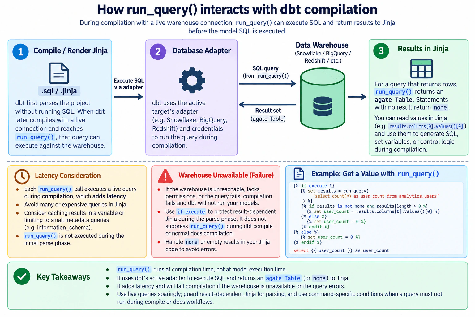
At a high level, run_query() lets Jinja read live warehouse data while dbt compiles with a connection. dbt sends the SQL through its active adapter, waits for the warehouse result, and makes that result available to Jinja. The initial parse phase does not run the query. The trade-off is that each live lookup adds latency and makes compilation dependent on warehouse availability, permissions, and query success.
This question is asking what happens when a project needs information from its database before the final work is ready to run. The key idea is that the project can ask the database for a value while it is being prepared, wait for the answer, and then use that answer to decide what to produce next. That makes the preparation more flexible, but it also creates a dependency on another system. If that system is slow, unavailable, or rejects the request, the preparation itself can slow down or fail.
Useful Questions to Ask the Interviewer
Should I distinguish dbt's initial parse phase from its compilation phase?
Should I cover both queries that return rows and statements that return no result?
Do you want me to include the latency and warehouse-availability impact of compilation-time queries?
How to Explain It in an Interview
1. Separate parsing from compilation
I would start by separating dbt's initial parse phase from compilation. During parsing, dbt reads the project and builds its dependency information, but it does not run SQL. At that point, execute is false. This matters because Jinja that expects live database results cannot safely assume those results exist during parsing.
2. run_query() executes when compilation reaches it with a live connection
When dbt later compiles a resource with a live warehouse connection, execute is true. If Jinja reaches run_query(), dbt can execute that SQL. In the diagram, Jinja sends the request toward the Database Adapter, and the adapter uses the active target connection and credentials to send the SQL query to the Data Warehouse. dbt waits for that query to complete before result-dependent Jinja can continue.
3. The warehouse result comes back into Jinja
For a query that returns rows, run_query() returns an agate Table. Jinja can read values from that table, assign them to variables, make decisions, or generate SQL from them. The diagram shows the result set flowing back from the Data Warehouse and becoming available in the Results in Jinja stage. If the statement does not return a result, run_query() returns none, so the Jinja logic must not blindly dereference a table result.
4. Use execute to protect parse-time result access
A common safe pattern is to put the live run_query() call and result-dependent logic inside an if execute branch. During the initial parse phase, execute is false, so that branch is skipped and a safe fallback can be used. During compilation, execute is true and the query can run. The important nuance is that if execute does not disable run_query() during dbt compile or normal documentation compilation. Those workflows compile the project with execute true, so reached run_query() calls can still access the warehouse.
5. Compilation now has latency and availability dependencies
Every run_query() call is a real warehouse query. That adds a database round trip and query execution time to compilation. Many calls or expensive queries can make compilation slower and consume warehouse resources. The warehouse also becomes part of the compilation dependency chain. If it is unreachable, credentials or permissions are invalid, or the SQL itself fails, compilation can fail before the model SQL is executed.
6. Use live compilation queries selectively
I would use run_query() when Jinja genuinely needs a small amount of live warehouse information to generate correct SQL or logic. The benefit is dynamic behavior based on current warehouse state. The downside is slower and more fragile compilation because an external system is now required. I would keep these lookups small, avoid unnecessary repetition, handle none or empty results, and use command-specific conditions when a query must not run during compile or documentation workflows.
Technical Approach
Let dbt complete its initial parse without relying on live database results.
During compilation, enter the live-query branch only when execute is true.
Call run_query() with the required SQL.
Let dbt's active adapter send that SQL to the target warehouse.
Wait for the warehouse response before continuing result-dependent Jinja rendering.
If the query returns rows, read the required value from the returned agate Table.
If no result is returned, handle none safely.
Use the obtained value to generate SQL or control Jinja logic.
Treat warehouse latency, connectivity, permissions, and query errors as compilation-time dependencies.
Practical Insights
The benefit is flexibility: Jinja can use information that already exists in the warehouse while dbt generates the final SQL. The downside is that compilation is no longer only local work. Every run_query() call requires a real database round trip, so additional calls create additional waiting and warehouse work. An expensive query can make compilation noticeably slower. Availability also matters because compilation may fail if the warehouse cannot be reached, credentials are invalid, permissions are missing, or the SQL fails. We accept this when the live value is genuinely needed to generate correct SQL. For a small lookup, the cost can be reasonable. For repeated or expensive queries, the latency and operational dependency can outweigh the convenience.
Code
template = """{# Do not perform live warehouse access during the initial parse phase. #}
{% if execute %}
{# Execute a small query during compilation and wait for its warehouse result. #}
{% set results = run_query(
'select count(*) as user_count from analytics.users'
) %}
{# Read the first returned value only when a usable result exists. #}
{% if results is not none and results|length > 0 %}
{% set user_count = results.columns[0].values()[0] %}
{% else %}
{# Use a safe fallback when no row result is available. #}
{% set user_count = 0 %}
{% endif %}
{% else %}
{# Parsing must not depend on a live warehouse result. #}
{% set user_count = 0 %}
{% endif %}
-- Use the Jinja value in the SQL generated by dbt.
select {{ user_count }} as user_count"""print(template)
Why Interviewers Ask This
Interviewers ask this to test whether a candidate understands that dbt compilation can depend on live external state instead of being only local text rendering. A strong answer separates parsing from compilation, explains how query results become available to Jinja, and recognizes the operational consequences: extra latency, warehouse permissions, availability, and query failures. It also tests judgment about when a dynamic database lookup is useful and when it makes compilation unnecessarily slow or fragile.
Common interview mistakes
A common mistake is saying that run_query() executes during dbt's initial parse phase. It does not; SQL is not run in that phase and execute is false. Another mistake is treating compilation as purely local or assuming model execution must happen before Jinja receives the run_query() result. Candidates may also assume every call returns a populated table, even though statements with no result return none and a result set can be empty. Another mistake is overlooking latency and availability: every call is a live warehouse operation. Finally, if execute should not be described as disabling run_query() during normal compilation, dbt compile, or ordinary docs compilation, because execute is true in those compilation workflows.
Interview tip
Lead with the phase distinction: parsing does not run the query, while compilation with a live connection can. Then trace the flow from Jinja to the Database Adapter to the Data Warehouse and back as an agate Table. Finish with the production trade-off: run_query() adds latency and makes compilation dependent on warehouse connectivity, permissions, and query success.
Interviewer may ask next
What changes if the warehouse is temporarily unavailable during compilation?
Compilation can fail because run_query() needs live warehouse access when the compilation path reaches that call. The changed requirement is availability: compilation now depends on the Data Warehouse being reachable and accepting the SQL sent through the Database Adapter. The initial parse phase is different because execute is false and the guarded live-query branch is skipped. During compilation, however, the warehouse dependency is real. If the connection fails, credentials are invalid, permissions are missing, or the query itself errors, Jinja cannot obtain the expected result and compilation may stop. I would keep the same design and expose the failure instead of inventing a production value. Result-dependent Jinja should still handle legitimate none or empty results separately. Recovery is to restore connectivity, correct permissions or SQL as appropriate, and rerun compilation. The downside is that a preparation step that might otherwise be local is now coupled to an external system's availability.
What if many models or macros start using run_query() during compilation?
The main concern becomes compilation latency and warehouse workload. The requirement that changes is scale: instead of one lightweight lookup, dbt may perform many live database round trips before model execution begins. The affected path remains Jinja to the Database Adapter to the Data Warehouse and back. Correctness rules stay the same: each result-producing query must return data in the form the Jinja logic expects, and none or empty results must be handled safely. I would keep the original design but reduce unnecessary repeated calls, keep the lookups small, and avoid expensive scans merely to generate SQL. If a query must not execute during compile or docs workflows, I would use a command-specific condition rather than relying only on if execute. Failures should remain visible rather than being silently converted into invented data. The downside of reducing live lookups is less dynamic behavior, but compilation becomes faster, cheaper, and less dependent on warehouse capacity.
26. What is distributed data processing, and why are data partitioning and shuffles important?Cloud / Distributed SystemsEasy
i Question Details
Define distributed data processing as coordinating computation across multiple processes or machines. Explain drivers or coordinators, workers or executors, partitions, task scheduling, data locality, shuffles, serialization, skew, retries, and fault recovery. Clarify that adding machines does not eliminate network, coordination, consistency, or workload-balance costs.
Short Interview Answer (30-60 seconds)
Distributed processing runs partition-level tasks across multiple workers under a coordinator. Partitions enable parallelism and locality, while shuffles redistribute records for operations such as grouping by key. Shuffles add network, serialization, coordination, and possible skew costs, so adding workers does not make those costs disappear.
Detailed Explanation
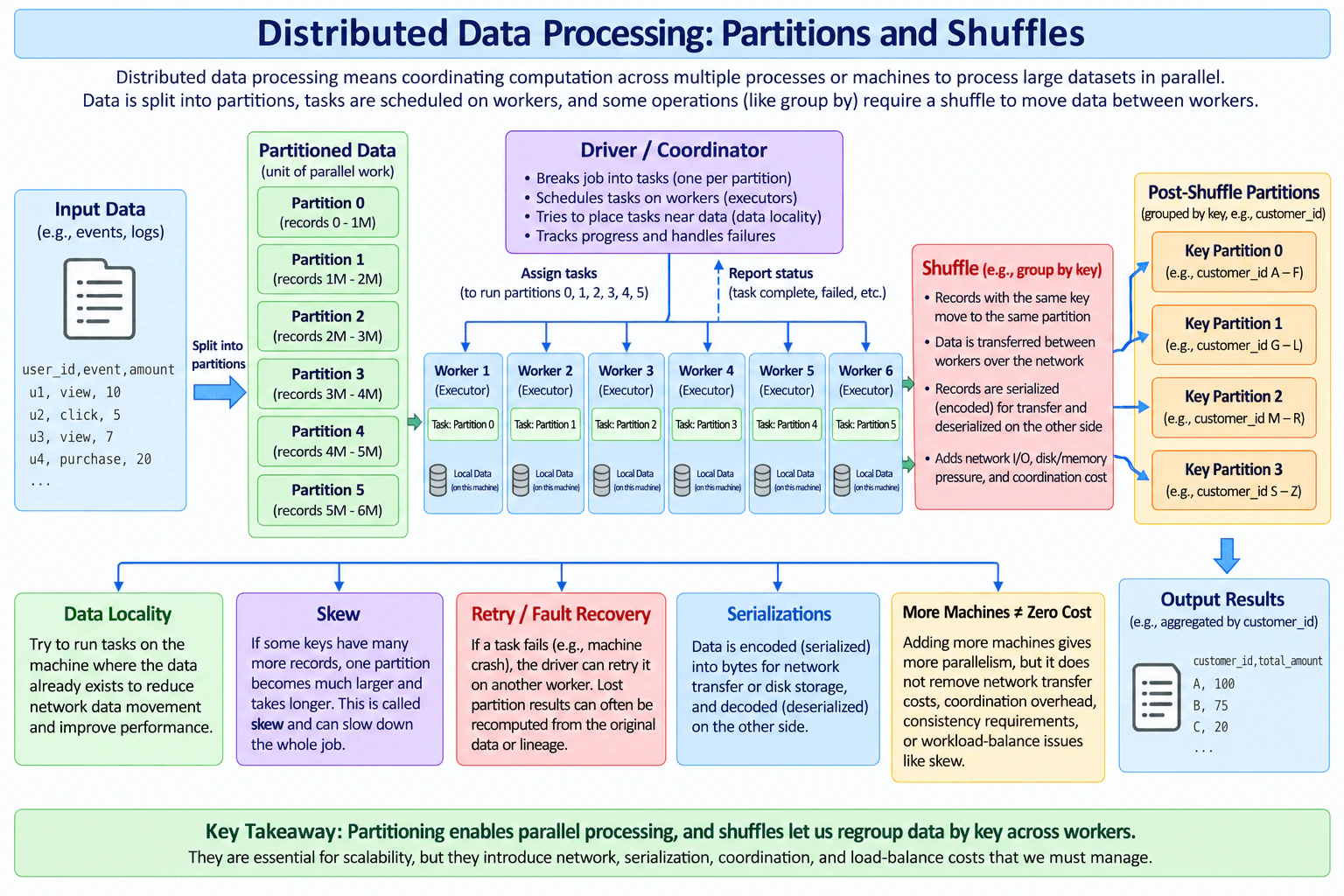
Distributed data processing means splitting a dataset into partitions and coordinating work on those partitions across multiple workers or machines. A driver or coordinator creates and schedules tasks, while workers execute those tasks, preferably near the data they need. In the diagram, six input partitions are assigned across six workers. Some operations can process each partition independently, but grouping records by a key requires a shuffle so matching keys move into the same post-shuffle partition. This enables correct distributed aggregation, but adds network transfer, serialization, coordination, possible disk or memory pressure, skew, retries, and recovery work.
Useful Questions to Ask the Interviewer
Is the question asking for a general distributed-processing explanation, or should I describe a particular processing engine?
Should I focus mainly on batch-style partition processing and shuffle behavior, as shown in this example?
Do you want me to discuss performance problems such as data skew, retries, and network overhead as part of the answer?
How to Explain It in an Interview
Start with the execution model. A driver or coordinator breaks the job into tasks and schedules those tasks on workers or executors. In the diagram, the input is divided into six partitions, numbered 0 through 5. The coordinator schedules one task for each of these partitions across the six illustrated workers and tracks status such as completion or failure.
Partitions are important because they define units of parallel work. Several partitions can be processed at the same time when resources are available. The scheduler can also try to place tasks near the data they need. The diagram calls this data locality: running a task where its partition already exists reduces unnecessary network movement and can improve performance.
A shuffle happens when the current partitioning no longer matches what the next operation requires. The diagram uses grouping by customer_id as the example. Records with the same key may initially exist on different workers, so they must be redistributed. During the shuffle, records are serialized into a transferable representation, sent between workers, and deserialized at the destination. After the exchange, records are placed into new key-based partitions, illustrated as customer_id ranges A-F, G-L, M-R, and S-Z, so related keys are routed to the appropriate downstream partition.
That shuffle is necessary for operations that require related records to be grouped, but it is expensive. It consumes network bandwidth and can put pressure on memory and local disk. Serialization and deserialization also consume CPU, and the exchange requires coordination across workers. Therefore, a job with a large shuffle can remain slow even when many workers are available.
Skew makes this worse. If some keys occur much more often than others, one post-shuffle partition can become much larger than the rest. The worker processing that partition takes longer and becomes a straggler while other workers finish earlier. The diagram therefore highlights workload balance as an important consideration rather than assuming every partition contains equal work.
Fault recovery is another part of distributed execution. If a task fails because a worker crashes or another execution failure occurs, the coordinator can retry the task on another worker. If an intermediate partition result is lost, it can often be recomputed from the original data or from the dependency lineage that produced it. Recovery preserves progress and correctness, but retries and recomputation add extra time and resource usage.
Finally, adding more machines only increases potential parallelism. It does not eliminate shuffle traffic, serialization, coordination, consistency requirements, retries, or uneven workload distribution. If the dominant cost is network movement or one skewed partition, additional workers may provide little improvement. The key interview point is that partitioning makes scalable parallel processing possible, while shuffles make cross-partition operations possible at a real communication, serialization, coordination, and load-balancing cost.
Technical Approach
1. Split the input dataset into partitions; the diagram uses partitions 0 through 5. 2. Let the driver or coordinator create partition-level tasks and schedule them on available workers. 3. Prefer data-local execution when possible so tasks run near the partitions they read. 4. Process each partition independently until an operation requires records to be regrouped across existing partition boundaries. 5. At that boundary, perform a shuffle: serialize records, transfer them between workers, and repartition them by the required key. 6. Process the new post-shuffle partitions and produce the aggregated output. 7. Watch for skew because hot keys can create oversized partitions and straggler tasks. 8. Retry failed tasks and recompute lost intermediate partitions when needed. 9. Evaluate network, serialization, coordination, memory, disk, and workload-balance costs before assuming additional machines will improve performance.
Practical Insights
CPU cost comes from processing records plus serialization and deserialization during exchanges. Memory is used for active task data and for organizing records during processing and shuffles; when memory is insufficient, local-disk work may increase. Network cost can become large because shuffle records move between workers. Local storage may hold intermediate data. Latency is often determined by the slowest task, so a skewed partition can delay the entire stage. More workers can increase parallelism, but communication and coordination remain. Distributed operation also adds recovery work such as retries and recomputation, so maintenance is more complex than processing everything on one machine.
Why Interviewers Ask This
Interviewers want to see whether you understand how distributed work is physically divided and coordinated rather than simply saying that more machines make processing faster. A strong answer connects partitions to task parallelism and locality, explains why grouping or similar operations create shuffle boundaries, recognizes serialization and network costs, identifies skew and stragglers, and explains retries and recomputation. It also shows judgment by recognizing that cluster scaling cannot eliminate communication, coordination, consistency, and workload-balance overhead.
Common interview mistakes
A common mistake is saying that distributed processing simply means adding more machines. Another is treating partitions only as storage chunks instead of units that determine task parallelism and data distribution. Candidates also often describe shuffles as free repartitioning and forget the network, serialization, memory, disk, and coordination costs. Another mistake is ignoring skew: having the same number of partitions does not mean each partition contains the same amount of work. It is also incorrect to assume every operation requires a shuffle; work that can consume an existing partition independently does not need cross-worker redistribution. Finally, do not claim that adding workers automatically fixes a slow job, because the bottleneck may be communication, skew, coordination, consistency requirements, or another shared resource.
Interview tip
Explain the flow in order: input partitions -> coordinator schedules tasks -> workers process partitions -> shuffle only when data must be regrouped -> new partitions -> result. Then mention locality, serialization, skew, retries, and why more machines do not remove distributed-system overhead.
Interviewer may ask next
Why can a shuffle become the slowest part of a distributed data-processing job?
A shuffle redistributes records across worker and partition boundaries. Records typically need to be serialized, transferred through the network, organized into new partitions, and deserialized for downstream processing. This adds CPU, network, memory, local-disk, and coordination work. It can become even slower when keys are unevenly distributed because one destination partition may contain much more data than the others, creating a straggler that delays completion of the stage.
Why does adding more workers not always make the job faster?
More workers increase potential parallelism only when there is enough independent and reasonably balanced work. They do not eliminate shuffle traffic, serialization, coordination, consistency requirements, retries, or skew. If one key creates a very large partition, the job may still wait for one slow worker. Likewise, if the dominant cost is moving data over the network, adding compute capacity does not remove that communication cost and can introduce additional coordination overhead.
27. How are assigned replicas and in-sync replicas different in Kafka?Cloud / Distributed SystemsEasy
i Question Details
Relate partition replica membership to replication progress and leader selection.
Short Interview Answer (30-60 seconds)
Assigned replicas are every broker configured to host a partition replica. ISR is the dynamic subset that is alive and keeping up with the leader. A lagging replica stays assigned but leaves ISR. ISR progress affects committed records, write availability, and leader selection.
Detailed Explanation
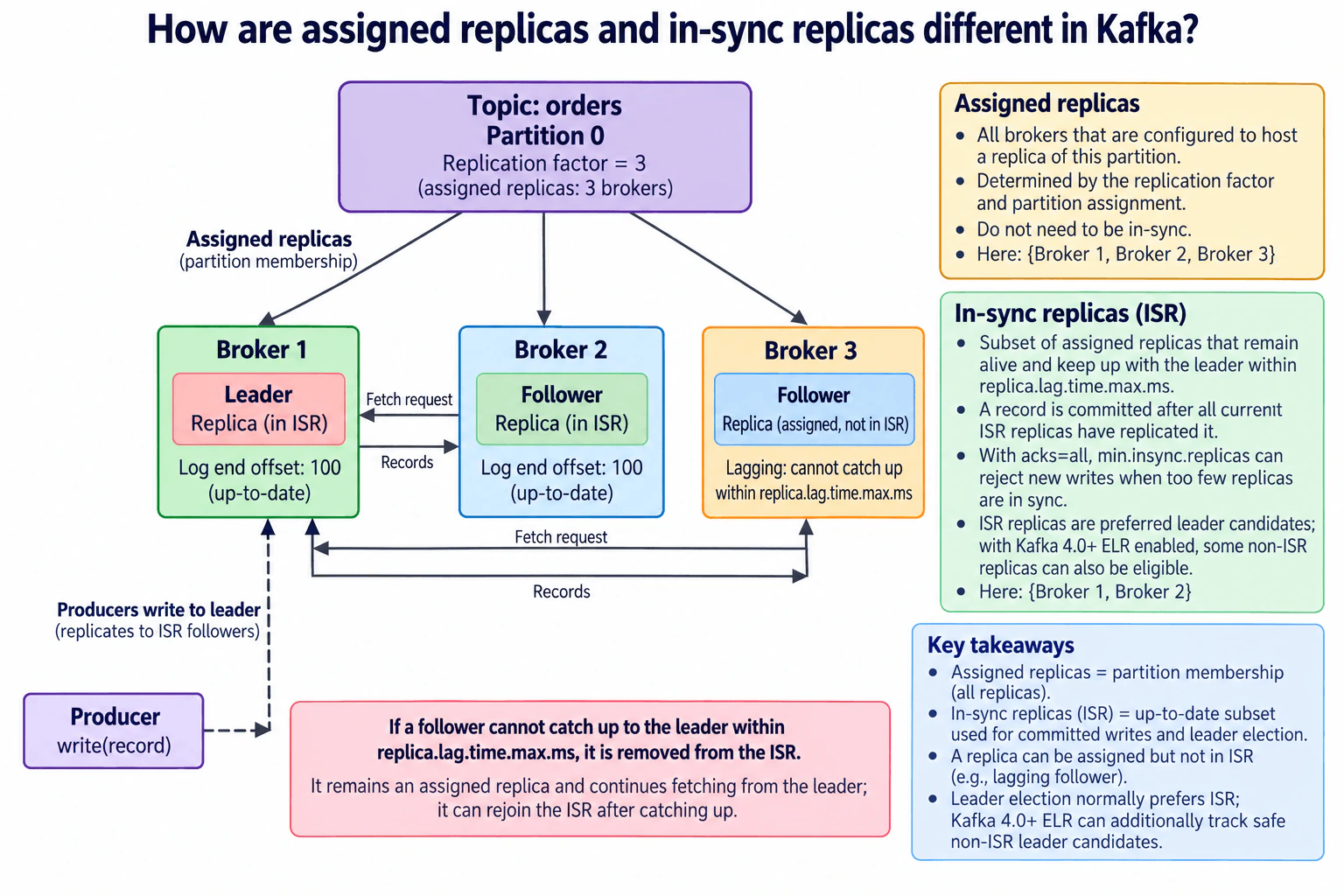
Assigned replicas define the full broker membership for a Kafka partition, while in-sync replicas (ISR) are the currently healthy assigned replicas that stay caught up with the leader within the allowed lag time. In the diagram, Partition 0 has three assigned replicas on Brokers 1, 2, and 3. Broker 1 is the leader, Broker 2 is an in-sync follower, and Broker 3 is still assigned but outside the ISR because it cannot catch up within replica.lag.time.max.ms. This distinction affects replication progress, record commitment, write availability, and leader election.
Useful Questions to Ask the Interviewer
Should I explain only the normal ISR behavior, or also mention Kafka 4.0+ Eligible Leader Replicas?
Do you want me to connect ISR membership to acks=all and min.insync.replicas?
Should I walk through what happens when an assigned follower falls behind and later catches up?
How to Explain It in an Interview
Start with membership. Partition 0 has replication factor 3, so its assigned replicas are Broker 1, Broker 2, and Broker 3. That assigned set describes where copies of the partition are configured to live. A broker does not stop being assigned just because its replica temporarily falls behind.
Next explain replication progress. Broker 1 is the leader. Broker 2 and Broker 3 are followers, and each follower fetches from Broker 1; the leader returns records to that follower. Broker 2 is alive and keeping up, so Broker 1 and Broker 2 are in the ISR. Broker 3 remains assigned but cannot catch up within replica.lag.time.max.ms, so it is outside the ISR. Kafka removes such a follower from the ISR, but the replica can keep fetching from the leader and can rejoin after it catches up.
The central distinction is therefore: assigned replicas are the full partition membership, while ISR is a dynamic subset representing replicas that are sufficiently current. In this example, assigned replicas are {Broker 1, Broker 2, Broker 3}, while ISR is {Broker 1, Broker 2}.
Replication progress also affects commitment. A record is committed after all current ISR replicas have replicated it. With acks=all, every current ISR replica participates in acknowledging the write, while min.insync.replicas sets the minimum ISR size required for that write to succeed. If the ISR becomes smaller than that minimum, Kafka can reject the write instead of accepting it with insufficient replication. kafka.apache.org
Leader election is also tied to replica state. When ISR is non-empty, Kafka chooses a leader from the ISR. With Kafka 4.0+ Eligible Leader Replicas enabled, the controller can additionally track certain non-ISR replicas as eligible candidates and may use ELR when ISR is empty. That matches the diagram's key point that ISR is normally preferred for leadership while ELR provides an additional safe candidate set in supported configurations. kafka.apache.org
For an interview, summarize it this way: assigned replicas answer 'which brokers host this partition?', while ISR answers 'which of those replicas are currently keeping up closely enough to participate in the partition's normal replication and preferred leader-selection behavior?'
Technical Approach
Identify the partition's full assigned replica set.
Identify the current leader.
Check which assigned followers remain alive and keep up with the leader within replica.lag.time.max.ms.
Treat the qualifying replicas, together with the leader, as the ISR.
If a follower cannot keep up within that time, remove it from ISR but keep it assigned and fetching from the leader.
Allow it to rejoin ISR after catching up.
Relate ISR progress to record commitment and relate acks=all plus min.insync.replicas to write availability.
For leader election, prefer ISR; when Kafka 4.0+ ELR is enabled, account for eligible non-ISR candidates as shown in the diagram.
Practical Insights
There is no useful Big-O complexity for this concept. The relevant costs are replication network traffic, disk storage for every assigned replica, and the latency required for followers to keep up with the leader. A higher replication factor consumes more storage and replication bandwidth but provides more redundancy. If ISR shrinks, lagging replicas continue using network and disk while catching up. With acks=all, a small ISR can also reduce write availability when min.insync.replicas is not satisfied. The operational trade-off is stronger replication safety versus availability during broker or network failures.
Why Interviewers Ask This
This question tests whether the candidate understands the difference between partition replica membership and dynamic replication progress. A strong answer should explain follower-to-leader replication, why a lagging replica can remain assigned but leave the ISR, how committed records relate to ISR progress, how min.insync.replicas affects acks=all write availability, and how replica state influences leader election.
Common interview mistakes
Common mistakes are treating assigned replicas and ISR as identical sets; assuming a lagging replica is removed from the partition assignment; drawing followers as replicating through one another instead of fetching directly from the leader; defining ISR only by an instantaneous equal log-end offset; confusing the commit condition with min.insync.replicas; assuming min.insync.replicas determines how many replicas acknowledge an acks=all write; and saying that only ISR replicas can ever be leader candidates without accounting for the Kafka 4.0+ ELR behavior shown in the approved diagram.
Interview tip
Use the diagram's small example: assigned replicas = {Broker 1, Broker 2, Broker 3}, ISR = {Broker 1, Broker 2}. Explain that Broker 3 is still a configured replica but is temporarily too far behind, then connect that distinction to replication progress, commitment, acks=all write availability, and leader election.
Interviewer may ask next
What happens when an assigned Kafka replica falls too far behind the leader?
It remains an assigned replica of the partition but leaves the ISR if it fails to keep up within replica.lag.time.max.ms. It continues fetching records from the leader, and after it catches up sufficiently it can rejoin the ISR.
How do acks=all and min.insync.replicas relate to ISR?
With acks=all, all replicas currently in the ISR must acknowledge the write for the producer request to succeed. min.insync.replicas sets the minimum ISR size that must be available for such a write. If the current ISR has fewer members than that minimum, Kafka rejects the write, trading write availability for the configured replication safety. kafka.apache.org
28. What happens during Kafka serialization and deserialization?Cloud / Distributed SystemsEasy
i Question Details
Trace the representation of a record from producer application data through broker storage to the consumer.
Short Interview Answer (30-60 seconds)
The producer serializes each record's key and value from application objects into byte arrays. Kafka transports and stores those serialized records in record batches. The consumer fetches the batches and uses compatible key and value deserializers to turn the bytes back into application objects.
Detailed Explanation
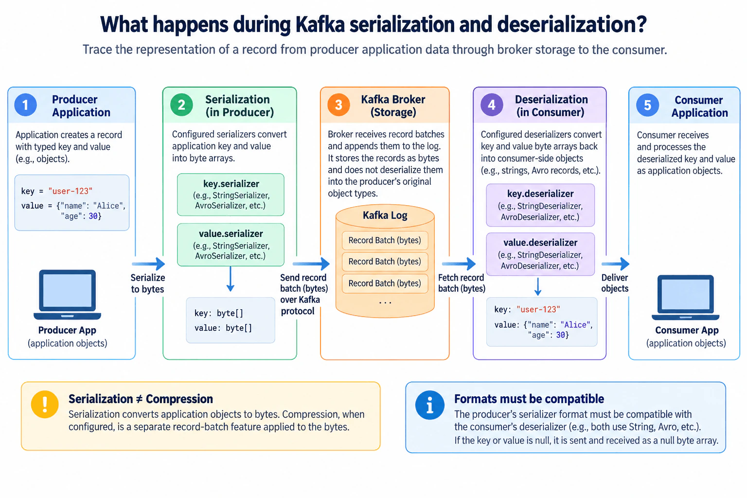
Kafka introduces a representation boundary between applications and the broker. A producer starts with application-side key and value objects. Its configured key serializer and value serializer convert those values into byte arrays. The producer then places serialized records into record batches and sends them to Kafka. The broker appends the serialized record data to its log; it does not reconstruct the producer's original object types. A consumer later fetches record batches, and its configured key and value deserializers convert the corresponding byte arrays into consumer-side objects that the application can process.
Useful Questions to Ask the Interviewer
Do you want me to explain the difference between serialization and record-batch compression?
Should I cover what happens when the producer and consumer use incompatible formats or schemas?
Should I include null keys and values as an edge case?
How to Explain It in an Interview
Start with the producer application. It creates a record whose key and value exist in the application's normal in-memory representation. In the diagram's example, the key is "user-123" and the value is a structured object containing fields such as name and age.
Next, the producer invokes the configured key serializer and value serializer. Each serializer converts its input into a byte-array representation. After this step, Kafka works with the serialized representation rather than the producer application's original object types.
The producer groups serialized records into record batches and sends those batches to the Kafka broker over the Kafka protocol. The broker receives the record batches and appends the serialized record data to the log. The important boundary is that the broker stores the record payload in serialized form; it does not deserialize the payload back into the producer application's original strings, domain objects, Avro records, or other application-side types.
When a consumer fetches a record batch, it receives records whose key and value are still represented as serialized bytes. The configured key deserializer and value deserializer perform the reverse application-side conversion: key bytes become a consumer-side key object, and value bytes become a consumer-side value object. The consumer application then processes those deserialized values.
Serialization and compression are different operations. Serialization converts an application key or value into bytes. Compression, when configured, is applied at the record-batch level to serialized record data. Compression can reduce the amount of data transferred and stored, but it does not replace the serializer or define the application's encoding contract.
The producer's serializer output must also be compatible with what the consumer's deserializer expects. If a producer encodes a value using one representation or schema but a consumer interprets those bytes using an incompatible representation, deserialization can fail or produce unusable data. The key and value have separate serialization and deserialization paths, so compatibility matters independently for each. A null key or value can remain null across this boundary rather than being converted into a normal non-null byte array.
Technical Approach
Begin with the producer application's key and value objects.
Apply the configured key serializer and value serializer to convert them into byte arrays.
Place serialized records into a record batch.
Send the record batch to the Kafka broker.
Append the serialized record data to the Kafka log without reconstructing application objects.
Have the consumer fetch the record batch.
Apply the configured key and value deserializers to reconstruct consumer-side objects.
Verify that the producer's encoding and the consumer's decoding expectations are compatible.
Treat optional record-batch compression as a separate concern from serialization.
Practical Insights
Serialization and deserialization use CPU because producers encode application objects into bytes and consumers decode bytes back into objects. Serialized records and record batches also occupy memory while they are buffered, transferred, and processed. Network transfer and broker storage operate on the serialized representation. Optional compression can reduce transferred and stored bytes, but compression and decompression add CPU work. The main operational risk is compatibility: if the producer changes its encoding or schema without keeping consumers compatible, consumers can encounter deserialization failures. The question provides no data sizes, throughput numbers, latency measurements, or cluster configuration, so no specific performance figures should be claimed.
Why Interviewers Ask This
Interviewers want to confirm that you understand the representation boundary between application objects and Kafka's byte-oriented transport and storage. A strong answer distinguishes producer-side serialization, broker-side storage of serialized records, consumer-side deserialization, and optional record-batch compression. It also explains why producer and consumer encoding expectations must remain compatible.
Common interview mistakes
Common mistakes include saying that Kafka brokers store producer application objects instead of serialized record data; treating serialization and compression as the same operation; forgetting that keys and values have separate serializers and deserializers; saying that brokers deserialize records into consumer objects; and ignoring format or schema compatibility between producers and consumers. Another mistake is assuming that changing a serializer on the producer has no effect on existing consumers.
Interview tip
Describe the record as a simple representation flow: producer objects -> serialized key/value bytes -> Kafka record batch and log -> fetched serialized bytes -> consumer objects. Then explicitly separate serialization from compression and mention producer-consumer format compatibility.
Interviewer may ask next
What happens if the producer serializer and consumer deserializer are incompatible?
The consumer still receives the serialized record data, but its deserializer may be unable to interpret the key or value according to the representation it expects. Deserialization can fail or yield unusable data. Producers and consumers therefore need a compatible encoding contract, including compatible schema expectations when a schema-based format is used.
Is Kafka serialization the same as Kafka compression?
No. Serialization converts an application's key or value into bytes. Compression is a separate operation applied to serialized records at the record-batch level when compression is configured. Serialization defines how application data becomes bytes, while compression reduces the size of the serialized batch representation.
29. When would you select LocalExecutor, CeleryExecutor, or KubernetesExecutor in Airflow?Cloud / Distributed SystemsMedium
i Question Details
Compare process placement, worker availability, task isolation, and startup overhead.
Short Interview Answer (30-60 seconds)
Use LocalExecutor for simple single-machine workloads, CeleryExecutor for distributed workloads that benefit from persistent workers and low task startup latency, and KubernetesExecutor when per-task isolation, custom resources, or elastic pod-based execution matter more than pod startup overhead.
Detailed Explanation
The key difference is where Airflow task processes run and what infrastructure must be available before execution. LocalExecutor starts task subprocesses on the scheduler machine, so it is simple and has very low startup overhead but shares one host. CeleryExecutor sends queued tasks through a message broker to persistent or autoscaled Celery workers, enabling distributed execution with low startup latency when workers are already running. KubernetesExecutor asks Kubernetes to create a separate pod for each queued task, providing stronger per-task isolation and flexible resources at the cost of pod startup latency.
Useful Questions to Ask the Interviewer
Is the Airflow deployment intended to remain on one machine, or must task execution scale across separate worker machines?
Do individual tasks need separate containers or different CPU, memory, image, or runtime requirements?
Is minimizing task startup latency more important than creating task workers dynamically?
Are persistent Celery workers already part of the operating model, or is Kubernetes the preferred execution platform?
How to Explain It in an Interview
Start with process placement. With LocalExecutor, the scheduler host also runs local task subprocesses. There is no separate worker fleet, so deployment and operation are comparatively simple. The trade-off is that task processes share the same host and therefore compete within that machine's CPU and memory limits. Startup overhead is very low because Airflow can start local subprocesses without dispatching the task to a remote worker or waiting for a Kubernetes pod. I would choose LocalExecutor for simple single-machine workloads where that host has enough capacity.
With CeleryExecutor, the scheduler queues work through a message broker, such as Redis, and Celery workers execute task processes on separate worker nodes. Those workers can be persistent, and worker autoscaling may be configured. When workers are already running and available, task startup is usually relatively quick because Airflow does not need to create a new execution container for every task. The trade-off is additional infrastructure: the broker and Celery worker fleet must be operated, and multiple tasks can share a worker host or container environment. I would choose CeleryExecutor for distributed workloads where warm workers and low task startup latency matter.
With KubernetesExecutor, the scheduler requests task execution through the Kubernetes API and each task instance runs in its own Kubernetes pod. Instead of maintaining a long-running Celery task-worker fleet, Kubernetes task pods are created for queued work. This provides strong per-task isolation and makes it practical to assign task-specific container images and resource requirements. The trade-off is startup latency because Kubernetes must schedule, create, and start the task pod before execution begins. I would choose KubernetesExecutor when per-task isolation, custom resources, or elastic pod-based execution are more important than minimizing task startup time.
The decision therefore comes down to the four dimensions shown in the diagram. LocalExecutor places task subprocesses on the scheduler machine, needs no separate worker fleet, shares the host, and has very low startup overhead. CeleryExecutor places tasks on separate Celery workers, can use persistent or configured autoscaled workers, provides distributed execution with shared worker infrastructure, and usually has low startup overhead when workers are warm. KubernetesExecutor places each task in its own dynamically created pod, provides the strongest per-task isolation of these three choices, and adds Kubernetes pod startup latency.
Technical Approach
Determine whether task execution can remain on the scheduler machine or must run on separate infrastructure.
Decide whether maintaining persistent workers is acceptable and useful for reducing task startup latency.
Determine whether tasks need per-task container isolation, different images, or custom CPU and memory requirements.
Compare startup behavior: local subprocess creation, dispatch to an available Celery worker, or Kubernetes pod creation.
Choose LocalExecutor for simple single-machine execution, CeleryExecutor for distributed execution with warm workers, or KubernetesExecutor for isolated and elastic pod-based execution.
Practical Insights
LocalExecutor has the least worker infrastructure and very low task-start overhead, but task CPU and memory consumption are concentrated on the scheduler machine. CeleryExecutor adds a message broker and worker fleet, increasing operational and maintenance work, but it distributes task execution across worker nodes and can start queued tasks quickly when workers are already available. KubernetesExecutor adds Kubernetes scheduling and pod-management overhead. Each task gets its own pod, which improves isolation and supports different resource requirements, but pod creation adds latency. These executors do not change the algorithmic complexity of the task itself; they mainly change execution placement, capacity, isolation, startup latency, and operational cost.
Why Interviewers Ask This
This question tests whether you understand how an Airflow executor changes where task processes run, what worker infrastructure must be available, how strongly tasks are isolated, and how much startup overhead is introduced. A strong answer connects those execution-model differences to practical deployment choices rather than treating one executor as universally better.
Common interview mistakes
A common mistake is saying KubernetesExecutor is always the best choice because it can scale. It also introduces Kubernetes operational complexity and pod startup latency. Another mistake is treating CeleryExecutor workers as if a new worker is created for every task; Celery workers normally exist independently of individual tasks and execute queued task processes. Also avoid saying LocalExecutor has a separate worker fleet: its task subprocesses run locally on the scheduler machine. Finally, do not equate distributed execution with per-task isolation. Celery tasks can share worker infrastructure, while KubernetesExecutor gives each task its own pod.
Interview tip
Structure the answer around the four requested dimensions: process placement, worker availability, task isolation, and startup overhead. Then map each executor to the workload that benefits from those trade-offs instead of simply ranking the executors.
Interviewer may ask next
Why might you choose CeleryExecutor instead of KubernetesExecutor for a high-volume Airflow deployment?
I would choose CeleryExecutor when I want distributed task execution but also want already-running workers to accept queued tasks with relatively low startup latency. The scheduler sends work through a broker to Celery workers on separate nodes. KubernetesExecutor creates a separate pod for each task, which provides stronger isolation and flexible per-task resources but introduces pod startup latency. For a steady workload where warm workers are desirable, CeleryExecutor can be the better fit.
When would LocalExecutor stop being a good fit?
LocalExecutor becomes less attractive when running task subprocesses on the scheduler machine no longer provides enough capacity or isolation. CPU and memory contention are concentrated on that host. If task execution needs to spread across separate worker nodes, CeleryExecutor provides a distributed worker model. If tasks also need separate containers, task-specific resources, or stronger per-task isolation, KubernetesExecutor is the more appropriate choice.
30. What does Kafka log compaction preserve, and what does it remove?Cloud / Distributed SystemsMedium
i Question Details
Explain how compaction changes what consumers can reconstruct about keyed state and its earlier history.
Short Interview Answer (30-60 seconds)
Kafka compaction keeps at least the latest record for each key and removes older superseded records. Surviving records keep their offsets and order. Tombstones represent deletions and may later disappear, so consumers can rebuild the latest keyed state, but not the complete history of earlier values.
Detailed Explanation
Kafka log compaction preserves keyed state rather than every historical update forever. For each key, Kafka retains at least the latest record while older records for that same key can be removed in the background. Records that survive keep their original offsets and relative ordering, so removed records create gaps instead of causing offsets to be renumbered. A record whose value is null acts as a tombstone for deletion. Consequently, a consumer replaying the compacted partition can reconstruct the latest keyed state that remains, but once superseded records are removed, it cannot reconstruct every earlier value that previously existed.
Useful Questions to Ask the Interviewer
Are we discussing a topic using log compaction rather than ordinary retention alone?
Should I include tombstone behavior and what happens when the tombstone itself is later removed?
Do you want me to focus on rebuilding current keyed state versus preserving complete change history?
How to Explain It in an Interview
Use the partition in the diagram as the example. Before compaction, key A appears three times: A=v1 at offset 0, A=v2 at offset 2, and A=v3 at offset 4. Because A=v3 is the newest value for A, compaction can remove A=v1 and A=v2 while retaining A=v3 at its original offset 4. Key B has B=b1 at offset 1 and no newer B record, so B=b1 remains.
Compaction does not renumber the records that survive. B=b1 remains at offset 1 and A=v3 remains at offset 4. The removed records therefore create offset gaps. The relative order of surviving records is also preserved; compaction removes records rather than reordering the ones that remain.
Key C demonstrates deletion. The partition first contains C=c1 at offset 3 and later contains C=null at offset 5. The null-valued record is a tombstone. It marks C as deleted and allows the earlier C=c1 record to be removed. The tombstone can itself later be removed after the configured delete-retention period. After both the old value and eventually the tombstone are gone, C contributes no value to the reconstructed current state.
A consumer replaying the compacted log from the beginning can therefore reconstruct the latest keyed state represented in the diagram: A=v3 and B=b1, with C deleted. What the consumer cannot reconstruct is the complete earlier history. Once A=v1 and A=v2 have been compacted away, for example, those intermediate states are no longer available from the compacted log.
The key interview distinction is that log compaction preserves enough information to rebuild the latest keyed state, while deliberately allowing older superseded history to disappear.
Technical Approach
Consider records within one Kafka partition as an ordered sequence of keyed updates with assigned offsets.
For each key, identify its newest record.
Retain at least that newest record while older records with the same key become eligible for removal.
Treat a null-valued record as a tombstone indicating that the key has been deleted.
Remove older values superseded by the tombstone; the tombstone may itself be removed later after the configured delete-retention period.
Keep the original offsets and relative ordering of records that survive, leaving gaps where records were compacted away.
Replay the remaining records from the beginning to reconstruct the latest keyed state.
Recognize that values already removed by compaction cannot be used to reconstruct the complete historical sequence of changes.
Practical Insights
Compaction is background broker work that reads and rewrites log segments, so it uses storage I/O, CPU, and temporary working resources. Its benefit is that obsolete versions of repeatedly updated keys do not need to remain indefinitely. Consumers rebuilding state can eventually read fewer obsolete records. Surviving offsets are unchanged, so applications must tolerate gaps. The main operational trade-off is retaining enough information for latest-state reconstruction while giving up the guarantee that every old version remains available for historical replay.
Why Interviewers Ask This
This question tests whether a Data Engineer understands the difference between Kafka as a history of changes and a compacted Kafka topic as a recoverable representation of keyed state. A strong answer explains latest-record preservation, removal of superseded values, tombstone deletion semantics, unchanged offsets, preserved ordering, offset gaps, and the consequence that compaction supports rebuilding current keyed state without preserving every earlier update.
Common interview mistakes
A common mistake is saying compaction immediately leaves exactly one record per key. Compaction runs in the background, so older versions can still exist until cleaning occurs; the important guarantee is that at least the latest value for each key is retained. Another mistake is saying surviving offsets are renumbered. They are not: removed records create gaps. Candidates also sometimes treat a null value as an ordinary value instead of a tombstone, or assume a tombstone remains forever. Finally, it is incorrect to say a compacted topic preserves complete history. After superseded records are removed, consumers can reconstruct the latest keyed state but cannot recover every earlier value from the compacted log.
Interview tip
Use the diagram's tiny example: A=v1, then A=v2, then A=v3. Explain that v1 and v2 may disappear while v3 stays at its original offset. Then mention the C tombstone and finish with the central distinction: latest keyed state is reconstructable, but complete value history is not.
Interviewer may ask next
Does Kafka log compaction renumber offsets after older records are removed?
No. A surviving record keeps the offset it received when it was written. If records at some earlier offsets are compacted away, those positions become gaps. A consumer reading through the partition advances to the next available record, while the relative order of the surviving records remains unchanged.
What happens to a key when Kafka receives a tombstone for it?
A tombstone is a record with the key and a null value. It marks that key as deleted and allows earlier values for the same key to be removed during compaction. The tombstone may itself later be removed after the configured delete-retention period. In the diagram, C=c1 is superseded by C=null, so C is absent from the reconstructed current state.
More questions load as you scroll
Disclaimer: This interview guide is for educational and informational purposes only. It is designed to help readers prepare, but it does not guarantee any interview result, hiring decision, offer, or outcome. Interview questions, hiring criteria, and preferred answers can vary by employer, interviewer, industry, location, and time. All answers, examples, and explanations in this guide are suggested examples for interview preparation, not definitive answers or instructions for professional practice. They are based on research and judgment, are provided without warranties of any kind, and should be adapted to the question, role, and applicable laws and professional requirements. Diagrams are simplified illustrations intended to highlight the main concepts and their relationships; actual situations, systems, and practices may be more complex. Alternative approaches may be equally valid or better suited to a particular question, context, or interviewer. To the fullest extent permitted by applicable law, the contributors and publisher are not liable for decisions made, actions taken, or losses incurred based on this guide.
State Laws and Professional Responsibilities: Laws and requirements governing an occupation vary by state and jurisdiction. You are responsible for checking the current laws, licensing requirements, and scope-of-practice rules that apply to your location and role, and for ensuring that your answers and actions comply with them. Adapt examples in this guide to those requirements. This guide is not legal advice.
Content Accuracy and Verification: To the fullest extent permitted by applicable law, we do not represent or warrant that interview guides, questions, answers, examples, or diagrams are accurate, complete, current, error-free, or suitable for any particular purpose. You are responsible for independently reviewing and verifying the information before relying on it.