This interview guide is for educational and informational purposes only. It is designed to help readers prepare, but it does not guarantee any interview result, hiring decision, offer, or outcome. Interview questions, hiring criteria, and preferred answers can vary by employer, interviewer, industry, location, and time. All answers, examples, and explanations in this guide are suggested examples for interview preparation, not definitive answers or instructions for professional practice. They are based on research and judgment, are provided without warranties of any kind, and should be adapted to the question, role, and applicable laws and professional requirements. Diagrams are simplified illustrations intended to highlight the main concepts and their relationships; actual situations, systems, and practices may be more complex. Alternative approaches may be equally valid or better suited to a particular question, context, or interviewer. To the fullest extent permitted by applicable law, the contributors and publisher are not liable for decisions made, actions taken, or losses incurred based on this guide.
State Laws and Professional Responsibilities
Laws and requirements governing an occupation vary by state and jurisdiction. You are responsible for checking the current laws, licensing requirements, and scope-of-practice rules that apply to your location and role, and for ensuring that your answers and actions comply with them. Adapt examples in this guide to those requirements. This guide is not legal advice.
Identity, Image, and Privacy Notice
To respect individual privacy, some names, profile photographs, avatars, biographical details, and other identifying information displayed in this guide may be replaced with pseudonyms, licensed stock images, illustrative avatars, composite images, or representative descriptions. Unless a person is expressly identified as an actual contributor, a displayed name, image, or profile should not be understood as depicting or identifying a specific candidate, interviewer, employee, or other real individual. These representations are provided for editorial and illustrative purposes only and do not imply endorsement, employment, participation, or affiliation with this guide or any company mentioned in it. Any resemblance to an actual person is coincidental.
Company Notice
This guide is an independent educational resource and is not affiliated with, endorsed by, sponsored by, or approved by the company named in this guide. Company names identify reported interview experiences or the employer context of clearly labeled original practice exercises. Interview practices can change without notice, and inclusion of company-specific content does not mean these questions are official, complete, or guaranteed to be asked. To the fullest extent permitted by law, the author, contributors, and publisher are not responsible for outcomes related to use of this material.
Content Accuracy and Verification
To the fullest extent permitted by applicable law, we do not represent or warrant that interview guides, questions, answers, examples, or diagrams are accurate, complete, current, error-free, or suitable for any particular purpose. You are responsible for independently reviewing and verifying the information before relying on it.
Questions or comments?
Contact us for general questions, or share feedback, technical corrections, and comments with the community.
11. How would you model vacation-rental bookings for booking-date acquisition metrics and stay-date revenue recognition?Data ModelingHard
i Question Details
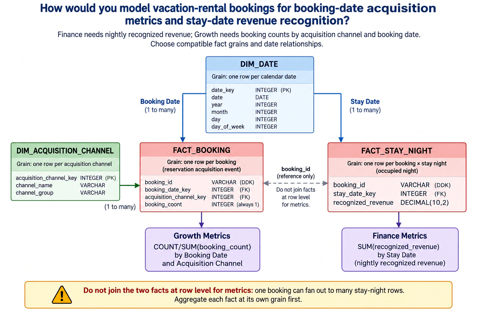
Finance needs nightly recognized revenue; Growth needs booking counts by acquisition channel and booking date. Choose compatible fact grains and date relationships.
Short Interview Answer (30-60 seconds)
I would use one booking-level fact for Growth and one booking-night fact for Finance. Both reference the same date dimension in different roles. Growth counts bookings by booking date and acquisition channel, while Finance sums recognized revenue by stay date. I would not join the raw facts for metrics.
Detailed Explanation
The company needs to answer two different business questions about the same reservation. Growth wants to know when a customer booked and which source brought that customer. Finance wants to know how much money belongs to each night of the stay. These events happen on different dates and at different levels of detail. If they are forced into one record, counts can repeat and money can be assigned to the wrong day. The clean design keeps booking activity and nightly stay activity separate while using one shared calendar so both teams report dates consistently.
Useful Questions to Ask the Interviewer
Should a reservation count once when it is created, even if it is changed or cancelled later?
Does recognized_revenue include only occupied nights, as shown in the model?
Is the acquisition channel fixed when the booking is created, or can attribution be restated later?
Which business time zone defines the booking date and stay date?
How to Explain It in an Interview
Start by declaring the grain of each fact table because that determines what can be counted or summed safely.
FACT_BOOKING has one row per booking, representing the reservation acquisition event. It contains booking_id, booking_date_key, acquisition_channel_key, and booking_count. In the diagram, booking_count is always 1. Growth can therefore calculate booking volume at this fact's grain and group it by Booking Date and Acquisition Channel.
booking_date_key is a foreign key to DIM_DATE. acquisition_channel_key is a foreign key to DIM_ACQUISITION_CHANNEL. DIM_ACQUISITION_CHANNEL has one row per acquisition channel, with acquisition_channel_key as the primary key and descriptive attributes such as channel_name and channel_group. One acquisition-channel row can relate to many booking rows.
FACT_STAY_NIGHT has a finer grain: one row per booking × stay night, representing an occupied night. It contains booking_id, stay_date_key, and recognized_revenue. Finance calculates nightly recognized revenue by summing recognized_revenue by Stay Date.
stay_date_key is a foreign key to the same DIM_DATE. DIM_DATE has one row per calendar date, with date_key as its primary key and attributes such as date, year, month, day, and day_of_week. The same conformed date dimension plays two logical roles: Booking Date for FACT_BOOKING.booking_date_key and Stay Date for FACT_STAY_NIGHT.stay_date_key. Each date row can relate to many rows in either fact.
The diagram also carries booking_id in both facts as a degenerate dimension key/reference. That shared identifier is useful for tracing a reservation across the two processes, but it should not be used to join the raw facts when calculating metrics.
The reason is fan-out. A single booking can produce several FACT_STAY_NIGHT rows. For example, one booking with four occupied nights produces one booking row but four stay-night rows. If the raw facts are joined by booking_id, the booking-level row is repeated four times. A booking count calculated after that join can therefore be overstated.
The safe rule is to aggregate each fact at its own grain first. Growth reads FACT_BOOKING and calculates booking counts by Booking Date and Acquisition Channel. Finance reads FACT_STAY_NIGHT and calculates SUM(recognized_revenue) by Stay Date. If a downstream report needs values from both processes, combine already-aggregated results only at a deliberately compatible reporting grain.
The tradeoff is that one reservation is represented at two grains, so the warehouse stores both a booking row and multiple nightly rows. That adds pipeline and storage work, but it makes the business meaning of each measure clear and prevents accidental double counting.
Technical Approach
Identify the two business processes: booking acquisition and nightly revenue recognition.
Declare FACT_BOOKING at one row per booking.
Store booking_date_key, acquisition_channel_key, booking_id, and booking_count = 1 in FACT_BOOKING.
Relate DIM_ACQUISITION_CHANNEL one-to-many to FACT_BOOKING.
Declare FACT_STAY_NIGHT at one row per booking × stay night.
Store stay_date_key, booking_id, and recognized_revenue in FACT_STAY_NIGHT.
Use one conformed DIM_DATE with booking_date_key and stay_date_key as separate logical date roles.
Calculate Growth metrics from FACT_BOOKING by Booking Date and Acquisition Channel.
Calculate Finance metrics from FACT_STAY_NIGHT by Stay Date.
Do not join the raw facts for metrics; aggregate each fact at its own grain before any combined reporting.
Practical Insights
The booking fact grows by one row for each reservation. The stay-night fact grows by one row for each occupied night, so a multi-night reservation creates several nightly rows. This means the nightly fact normally requires more storage and more processing. In return, Growth and Finance queries remain simple because each measure lives at the level where it is valid. The main operational cost is maintaining two related pipelines and consistent date-key lookups. The maintenance benefit is clearer metric ownership and a much lower risk of double counting.
Why Interviewers Ask This
This question tests whether the candidate can declare the correct fact-table grains for two related business processes, use a conformed date dimension in multiple roles, place measures at the grain where they are valid, model acquisition-channel relationships correctly, and recognize the fan-out problem caused by joining a booking-level fact directly to a nightly fact.
Common interview mistakes
A common mistake is using one booking-level row for both acquisition metrics and nightly revenue, which makes stay-date recognition difficult. Another is expanding every booking into nightly rows and then counting those nightly rows as bookings, which overcounts multi-night reservations. A third mistake is joining FACT_BOOKING directly to FACT_STAY_NIGHT by booking_id and then calculating booking-level measures, because one booking can fan out to many nightly rows. It is also incorrect to group recognized revenue by Booking Date instead of Stay Date, or to group acquisition counts by Stay Date instead of Booking Date. Finally, using separate inconsistent calendar dimensions for the two date roles can cause reporting definitions to drift.
Interview tip
Lead with the two grains: one row per booking for Growth and one row per booking × stay night for Finance. Then explain the Booking Date and Stay Date roles of the shared date dimension. Finish by calling out the raw-fact fan-out problem and the rule to aggregate each fact first.
Interviewer may ask next
How would you combine booking counts and recognized revenue in one dashboard without double counting?
Aggregate the two facts independently before combining them. Calculate booking metrics from FACT_BOOKING at the required Booking Date and Acquisition Channel grain. Calculate revenue metrics from FACT_STAY_NIGHT at the required Stay Date grain. If a dashboard needs both values together, first bring each result to a deliberately compatible reporting grain through the appropriate shared dimensions. Do not join the raw fact rows by booking_id, because a multi-night booking would repeat the booking-level measures.
Why not store all recognized revenue only on the booking-level fact and allocate it when reports run?
Finance needs recognized revenue by individual stay date, so the nightly allocation is part of the measure's required grain. Storing recognized_revenue directly in FACT_STAY_NIGHT makes it additive by Stay Date and avoids repeating allocation logic in every report. The booking fact can still represent the acquisition event, but it should not replace the nightly fact when nightly revenue recognition is the requirement.
12. How would you model Snowflake cost per query by team and day?Data ModelingHard
i Question Details
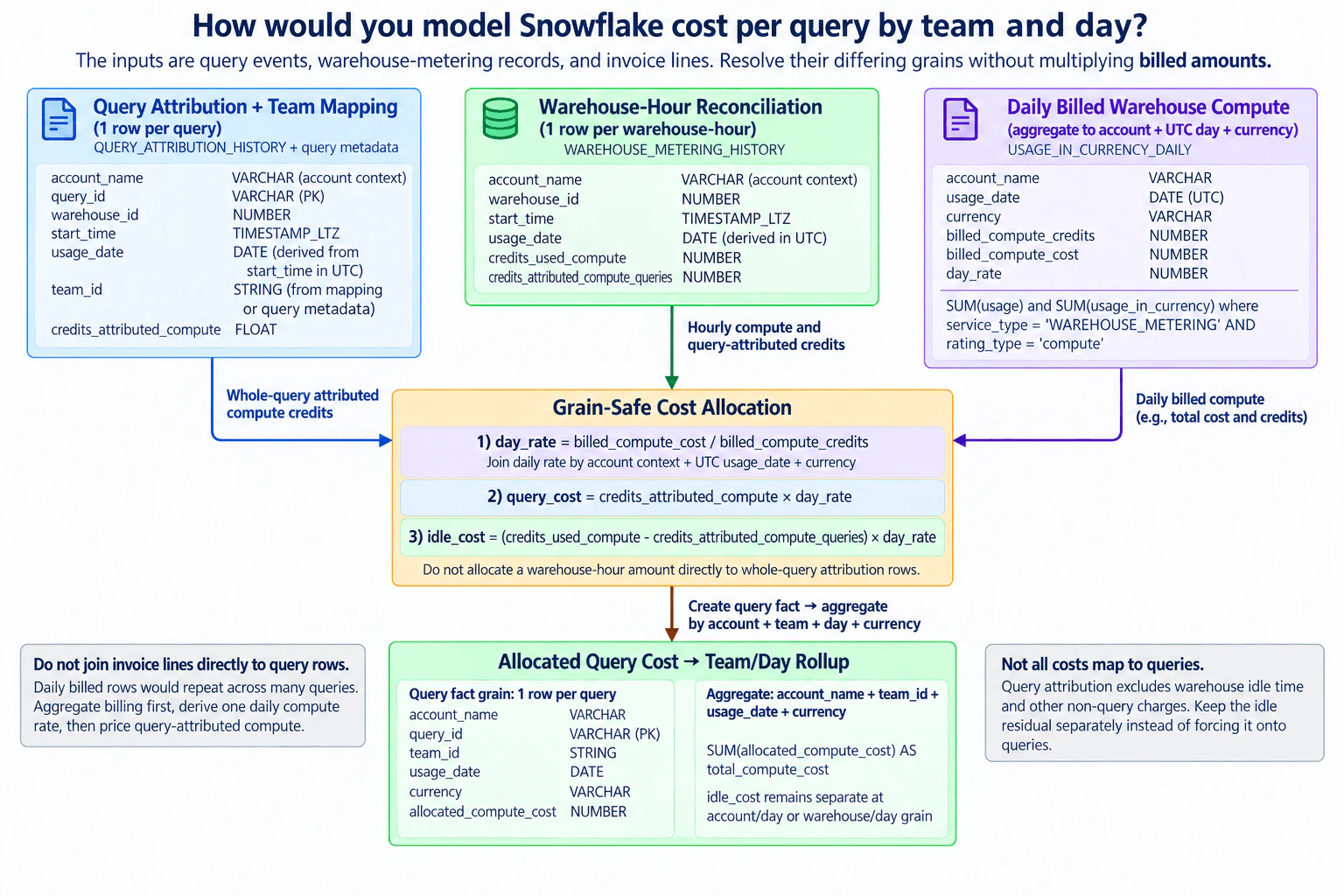
The inputs are query events, warehouse-metering records, and invoice lines. Resolve their differing grains without multiplying billed amounts.
Short Interview Answer (30-60 seconds)
I would derive one billed compute rate per account, UTC day, and currency, apply it to each query's attributed compute credits, keep warehouse idle cost separate, and aggregate the resulting one-row-per-query cost fact by team and day.
Detailed Explanation
The three inputs describe the same spending at different levels. One describes each request, one shows machine use by hour, and one contains the amount charged for a day. If the daily charge is copied onto every request, the same money can be counted many times. I would first calculate one trusted daily price, use it to value each request once, keep unused machine time separate, attach each request to its team, and then add the request costs by team and day. This keeps the totals consistent with the original bill.
Useful Questions to Ask the Interviewer
Should the result include only virtual-warehouse compute, as shown in the diagram, or other Snowflake charges too?
Where should team ownership come from: query metadata, a maintained mapping, or another source?
Should each billing currency remain separate in the final metric?
Should warehouse idle cost remain a separate residual, or should a later business rule allocate it to teams?
Should a query be assigned to the UTC date derived from its start_time, including queries that cross midnight?
How to Explain It in an Interview
I would start by declaring the grain of every source.
Query Attribution + Team Mapping has one row per query. It is based on QUERY_ATTRIBUTION_HISTORY plus query metadata. The modeled fields are account_name as account context, query_id, warehouse_id, start_time, usage_date derived from start_time in UTC, team_id, and credits_attributed_compute. The key point is that credits_attributed_compute represents compute attributed to the whole query, not an hourly query measure.
Warehouse-Hour Reconciliation has one row per warehouse-hour from WAREHOUSE_METERING_HISTORY. It contains account_name as account context, warehouse_id, start_time, usage_date derived in UTC, credits_used_compute, and credits_attributed_compute_queries. The difference between credits_used_compute and credits_attributed_compute_queries represents warehouse compute that was not attributed to queries for that hour.
Daily Billed Warehouse Compute is aggregated from USAGE_IN_CURRENCY_DAILY to account plus UTC day plus currency. For this model, filter to service_type = 'WAREHOUSE_METERING' and rating_type = 'compute'. Calculate billed_compute_credits = SUM(usage) and billed_compute_cost = SUM(usage_in_currency). Then derive day_rate = billed_compute_cost / billed_compute_credits.
The cost allocation is grain-safe. The billing source alone determines the daily rate. Join that rate by account context, UTC usage_date, and currency. For each whole-query attribution row, calculate query_cost = credits_attributed_compute * day_rate. Separately, calculate hourly idle cost as (credits_used_compute - credits_attributed_compute_queries) * day_rate.
Do not allocate a warehouse-hour amount directly to whole-query attribution rows. They have different grains. The daily rate is the common pricing measure that can be applied independently to query-attributed credits and idle credits.
The resulting query-cost fact has one row per query with account_name, query_id, team_id, usage_date, currency, and allocated_compute_cost. The final metric groups by account_name, team_id, usage_date, and currency, then calculates SUM(allocated_compute_cost) AS total_compute_cost.
Idle cost remains separate at account/day or warehouse/day grain and is not included in the team query-attributed total. One explicit tradeoff is the day assignment for queries that cross UTC midnight: this diagram assigns the whole query to the UTC date derived from start_time. If exact cross-day allocation were required, the model would need a finer-grained query attribution source or another documented allocation rule.
Technical Approach
Keep query attribution at one row per query and attach team_id, account context, and usage_date derived from start_time in UTC.
Keep warehouse metering at one row per warehouse-hour with credits_used_compute and credits_attributed_compute_queries.
Filter billing to service_type = 'WAREHOUSE_METERING' and rating_type = 'compute'.
Aggregate billing by account, UTC day, and currency to produce billed_compute_credits = SUM(usage) and billed_compute_cost = SUM(usage_in_currency).
Calculate day_rate = billed_compute_cost / billed_compute_credits; treat a zero or missing denominator as an exception rather than dividing by zero.
Join the daily rate to query attribution using account context, UTC usage_date, and currency.
Calculate query_cost = credits_attributed_compute * day_rate for each query.
Join the same daily rate to warehouse-hour reconciliation and calculate idle_cost = (credits_used_compute - credits_attributed_compute_queries) * day_rate.
Persist one query-cost fact row per query.
Aggregate allocated_compute_cost by account, team, UTC day, and currency while leaving idle cost outside the query-attributed team total.
Practical Insights
The largest dataset is usually the query-cost fact because it keeps one row for every query. Warehouse-hour data is smaller, and daily billing data is much smaller. Processing mainly requires filtering billing rows, grouping them by account/day/currency, deriving UTC dates, joining a small daily-rate result to query and warehouse facts, and grouping query costs by team and day. Ongoing maintenance mainly involves correct team mappings, consistent UTC handling, currency separation, missing-rate handling, and checks that prevent daily billing rows from being duplicated.
Why Interviewers Ask This
This question tests whether the candidate recognizes incompatible data grains and prevents fan-out that multiplies billed amounts. It also evaluates fact-table grain, allocation rules, UTC date alignment, team attribution, billing reconciliation, additive measures, and the distinction between whole-query attributed compute and warehouse idle compute.
Common interview mistakes
Common mistakes are joining daily invoice rows directly to query rows and multiplying the same billed amount; treating whole-query credits_attributed_compute as an hourly measure; feeding query or warehouse-hour facts into the daily-rate calculation instead of deriving the rate only from billing; mixing local dates with the UTC billing day; omitting account context or currency from the rate relationship; including unrelated service types in the warehouse-compute rate; forcing idle cost into the query-cost fact; dividing by zero when billed compute credits are zero; combining different currencies without conversion; and ignoring the start-date allocation tradeoff for queries that cross UTC midnight.
Interview tip
Lead with the grain mismatch and fan-out risk. State the three source grains, derive one daily billed compute rate only from billing, apply that rate separately to whole-query credits and idle credits, and finish with the one-row-per-query fact and team/day rollup. Explicitly say that daily billed rows are never joined directly to queries.
Interviewer may ask next
How would you handle warehouse idle cost if the business wants every compute dollar assigned to a team?
Keep the measured idle residual separate first so reconciliation stays auditable. If the business requires allocation, add an explicit policy after the direct query-cost calculation. For example, distribute an account-day or warehouse-day idle amount across teams according to their query-attributed compute share. Store that policy-based amount separately from direct query cost so users can distinguish measured attribution from allocated idle overhead.
How would you handle a query that runs across two UTC days?
In the diagram's model, the whole query is assigned to the UTC usage_date derived from start_time, so its attributed compute is priced using that day's rate. That is a documented modeling tradeoff. If the requirement is exact daily reconciliation for cross-midnight queries, I would need finer-grained query attribution by time interval or an explicit rule that splits the query's attributed credits across days before applying each day's rate.
13. What is a data pipeline, and how do orchestration, ETL, and ELT fit into it?Data PipelinesEasy
i Question Details
Define a data pipeline as a repeatable flow that moves and processes data from sources to consumers. Explain extraction, validation, transformation, loading, dependencies, schedules or event triggers, retries, idempotency, checkpoints, backfills, observability, and data contracts. Distinguish ETL from ELT and orchestration from the work performed by each task.
Short Interview Answer (30-60 seconds)
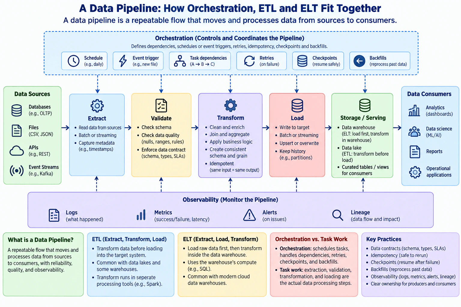
A data pipeline is a repeatable flow that moves and processes data from sources to consumers. In this design, data is extracted, validated, transformed, loaded, stored, and then served to analytics, data science, reports, or applications. Orchestration coordinates schedules or events, dependencies, retries, recovery checkpoints, and backfills, while tasks perform the actual data work. ETL transforms before loading; ELT loads first and transforms in the target. Idempotency makes retries and backfills safer.
Detailed Explanation
A data pipeline is a repeatable way to move information from where it is created to where people or applications can use it. The flow can begin with databases, files, APIs, or event streams. The information is read, checked for problems, changed into a useful form, stored, and then made available for analysis, reports, models, or applications. A separate control layer decides when work should start, which step depends on another step, and how failed or historical work should be run again safely.
Useful Questions to Ask the Interviewer
Should the pipeline run on a fixed schedule, from an event trigger, or support both?
Is the expected processing batch, streaming, or a mixture of both?
Should I explain both ETL and ELT, or is one pattern preferred for the target system?
What reliability expectations matter most for retries, backfills, checkpoints, and duplicate prevention?
How to Explain It in an Interview
1. Start with sources and extraction
I would start with the big picture: the pipeline moves data from producers to downstream consumers in a repeatable way. The diagram shows databases, files, APIs, and event streams as example sources. The Extract task reads from those sources. It can work with batch or streaming input and captures useful metadata such as timestamps. The extracted data then moves to validation before later processing depends on it.
2. Validate the data contract
The Validate task checks that incoming data has the expected structure and quality. In the diagram, this includes schema checks, type checks, null or range rules, and enforcement of a data contract. A data contract is an agreement about the schema, types, service expectations, and other rules that producers and consumers rely on. A workflow can finish technically while still producing bad data, so validation is separate from orchestration state. Valid data then moves to transformation.
3. Transform the records and make reruns safe
The Transform task cleans and enriches data, performs joins or aggregation, applies business logic, and creates a consistent schema and grain. Grain means what one record represents. The diagram also calls out idempotency: repeating the same processing should produce the same intended result rather than creating unintended duplicates. This is important because a failed task may be retried and historical data may later be processed again during a backfill.
4. Load and serve the result
The Load task writes data to the target. The diagram allows batch or streaming writes and shows upsert or overwrite as possible write behaviors. It can also keep history, for example through partitions. The result then appears in the Storage / Serving layer, which shows a data warehouse, data lake, or curated tables and views. From there, consumers such as analytics dashboards, data-science workloads, reports, and operational applications can use the data.
5. Distinguish ETL from ELT
ETL means Extract, Transform, Load. The transformation happens before data is loaded into its final target. ELT means Extract, Load, Transform. Raw or lightly processed data is loaded first, and transformation happens later inside the target system, often using the target system's compute. The pipeline concept is broader than either pattern. ETL and ELT simply place the transformation step at different points in the overall data flow.
6. Separate orchestration from task work
Orchestration is the control layer above the main data path. It coordinates when work runs and in what order, while the individual tasks perform extraction, validation, transformation, and loading. The diagram shows fixed schedules, event triggers, task dependencies, retries after failure, checkpoint-based recovery, and backfills for historical data. A retry repeats failed work. A backfill intentionally processes earlier data. Checkpoints record processing progress so supported workloads can resume safely. Idempotent task behavior is important because the same work may run more than once.
7. Observe and operate the pipeline
Observability is separate from the main business-data path. The diagram shows logs for what happened, metrics such as success, failure, and latency, alerts when problems occur, and lineage for understanding where data came from and what downstream data may be affected. These signals help operators detect failures and verify recovery. Together with data contracts, idempotency, checkpoints, backfills, and clear producer and consumer ownership, observability makes the pipeline easier to trust and operate.
Technical Approach
Identify the source systems and downstream consumers.
Define the data contract, including expected schema, types, grain, and quality rules.
Extract data from databases, files, APIs, or event streams using the required batch or streaming behavior.
Validate schema and data quality before downstream processing.
Transform the data through cleaning, enrichment, joins, aggregation, and business logic while keeping reruns idempotent.
Load the accepted result into the target and expose warehouse, lake, or curated serving structures.
Use orchestration to coordinate schedules or event triggers, dependencies, retries, checkpoint-aware recovery, and backfills.
Monitor logs, metrics, alerts, and lineage so failures and downstream impact can be understood.
Practical Insights
The benefit is that responsibilities are clear: processing tasks move and change data, while orchestration coordinates their execution. Batch processing is usually simpler to operate, but the data may be less fresh. Streaming can reduce latency, but checkpoints, recovery, and monitoring become more important. Strong validation catches bad data earlier, but it can delay delivery when records fail checks. Idempotent writes make retries and backfills safer, but they may require stable keys and careful upsert or overwrite logic. Keeping history in partitions can make replay and backfill easier, but it increases storage and maintenance. We accept these costs because reliable recovery and trustworthy data are usually more important than having the simplest possible pipeline.
Why Interviewers Ask This
Interviewers ask this to see whether you understand both data flow and control flow. They want to know if you can explain how data moves from sources to consumers, where validation and transformation happen, and how workflow execution is coordinated. They also test whether you can distinguish ETL from ELT, separate orchestration from task work, and reason about data contracts, idempotency, retries, checkpoints, backfills, observability, lineage, and safe recovery.
Common interview mistakes
Common mistakes are saying that the orchestrator itself performs extraction, validation, transformation, or loading, or treating monitoring as part of the business-data path. Another mistake is confusing ETL and ELT: their main difference is whether transformation happens before or after loading into the target. Candidates also confuse retries with backfills. A retry repeats failed work, while a backfill intentionally processes historical data. Other mistakes include ignoring idempotency when work can repeat, treating task success as proof of correct data, skipping data-contract and quality checks, or describing checkpoints as a universal orchestrator guarantee instead of processing progress used for supported recovery.
Interview tip
Follow the diagram from left to right. Start with sources, then explain Extract, Validate, Transform, Load, Storage / Serving, and consumers. Next separate the orchestration control layer from the task work. Explain ETL versus ELT with one clear sentence about where transformation happens. Finish with reliability and operations: idempotency, retries, checkpoints, backfills, data contracts, logs, metrics, alerts, and lineage.
Interviewer may ask next
How would the design change if the business needed much fresher data instead of a daily batch?
I would keep the same overall pipeline responsibilities but use the streaming behavior already shown in the design where it is needed. The main requirement that changes is freshness. Instead of waiting for one large scheduled batch, extraction and loading can process records continuously or in smaller units as data arrives. Validate and Transform still enforce the same schema, quality, business logic, and grain rules. Orchestration can use an event trigger and continue managing dependencies and failed task execution, but it does not become the component that processes each record. Checkpoints become more important because a streaming workload needs a known progress position for recovery. Idempotent output is still required so repeated work does not create incorrect duplicate results. Logs, latency metrics, alerts, and lineage keep the same purpose. The main downside is operational complexity: streaming generally needs more careful recovery, state handling, monitoring, and sink behavior than a simple scheduled batch.
What happens if a transformation fails after some data has already been processed?
I would mark the Transform task as failed and use the existing recovery behavior rather than treating the workflow as successfully complete. The affected flow is Transform followed by its dependent Load step. Orchestration can coordinate a retry of the failed work. The important correctness rule is idempotency: repeating the transformation must lead to the same intended result rather than creating unintended duplicates. If the workload supports checkpoints, the processing layer can use recorded progress to resume from a safe point instead of assuming that all input must restart. Validation still applies before the recovered result is trusted. If a historical period needs to be processed intentionally, I would use a backfill rather than call it a retry. Logs show what happened, metrics and alerts expose the failure, and lineage helps identify downstream impact. The downside is that safe recovery requires additional state, metadata, and operational discipline.
14. Why does a daily Airflow data-interval run for Monday start on Tuesday?Data PipelinesEasy
i Question Details
Relate the run’s logical date to the start and completion of its daily data interval.
Short Interview Answer (30-60 seconds)
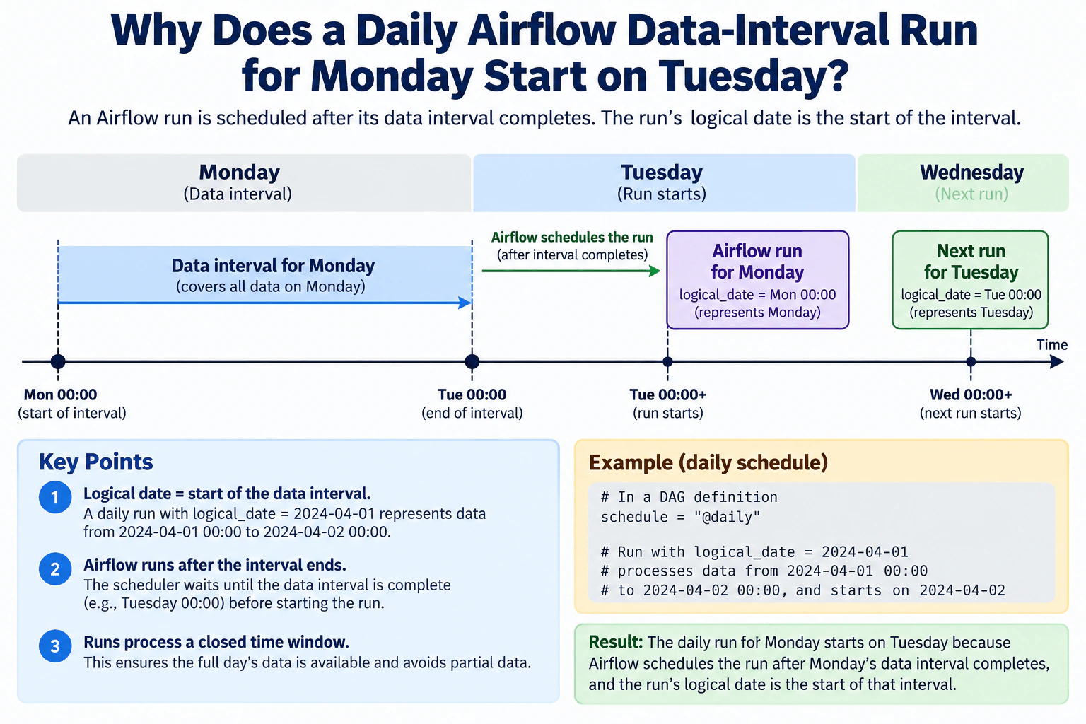
A daily Airflow run represents a completed daily data interval. Monday's interval starts at Monday 00:00 and ends at Tuesday 00:00. Airflow schedules that interval's run after the interval has ended, so the Monday run begins on Tuesday. Its logical date is still Monday 00:00 because the logical date identifies the start of the interval being processed. The benefit is a complete daily window; the trade-off is waiting until that window finishes before processing it.
Detailed Explanation
The question asks why work for Monday is started on Tuesday. Think of Monday as one complete box of time. The box opens at midnight on Monday and closes at midnight on Tuesday. The system waits until the box has finished before starting the work for it. Even though the work begins on Tuesday, it is still associated with Monday because Monday is when that box began. The important idea is that the date attached to the work identifies the period being handled, not the exact clock time when the work begins.
Useful Questions to Ask the Interviewer
Should I assume the DAG uses a normal interval-based daily schedule such as @daily?
Should I distinguish the run's logical date from its actual wall-clock start time?
How to Explain It in an Interview
1. Define the Monday data interval
I would start by saying that the Airflow run represents a data interval. In the diagram, Monday's interval begins at Monday 00:00 and ends at Tuesday 00:00. It represents the complete Monday window. For a daily interval schedule, this is the period whose data the run is associated with.
2. Wait for the interval to complete
The scheduler does not schedule that interval's run at the beginning of Monday. It waits until the Monday interval has completed. That boundary occurs at Tuesday 00:00. The diagram therefore shows the scheduling control flow moving from the completed Monday interval toward the Monday Airflow run on Tuesday.
The actual run may begin just after the boundary, shown as Tuesday 00:00+ in the diagram. The important rule is that the interval has finished before the scheduled run is created and started; it does not mean task execution must occur at the exact midnight instant.
3. Use the interval start as the logical date
The Monday run has logical_date = Mon 00:00. That logical date identifies the beginning of the interval represented by the run. It is not the physical execution start time.
This is the key interview distinction: Monday 00:00 tells us which daily interval the run represents, while Tuesday tells us when that completed interval becomes eligible for its scheduled run.
4. Apply the same rule to Tuesday
The next interval begins at Tuesday 00:00 and ends at Wednesday 00:00. Its run therefore starts on Wednesday 00:00+ in the diagram, while its logical date is Tuesday 00:00.
That repeating pattern is a useful correctness check: the interval start becomes the logical date, and the run is scheduled after the interval reaches its end boundary.
5. Explain the practical trade-off
The benefit is a clear, completed daily window. A run labeled for Monday consistently represents Monday's interval instead of an incomplete part of that day. The downside is freshness: Monday's scheduled daily processing cannot begin until the Monday interval reaches its Tuesday boundary.
A concise interview summary is: the logical date names the start of the data interval, while the run is scheduled after that interval completes. That is why the Monday run starts on Tuesday.
Technical Approach
Identify the daily data interval represented by the run.
Mark its start and end boundaries.
Treat the interval start as the run's logical date.
Recognize that the interval-based daily run is scheduled after the interval ends.
Keep the logical date separate from the actual wall-clock run start.
Apply the same rule to the next daily interval to verify the pattern.
Practical Insights
There is no meaningful algorithmic time or memory complexity to calculate because this question is about scheduling behavior. The relevant trade-off is freshness. The benefit is that each daily run represents one completed and clearly defined daily interval, which makes the meaning of the run easy to reason about. The downside is that Monday's scheduled processing waits until the Monday interval ends at Tuesday 00:00 before that run becomes schedulable. We accept this because the design is intentionally based on completed daily windows. Operationally, engineers must also remember that the logical date identifies the interval start; it is not a promise about the exact wall-clock time when the scheduler or tasks begin running.
Why Interviewers Ask This
Interviewers ask this to test whether you understand the difference between the time period a scheduled run represents and the time when that run actually begins. A strong answer shows that you can reason about daily interval boundaries, explain the meaning of Airflow's logical date, and avoid treating the logical date as the wall-clock execution time. The question mainly tests scheduling semantics and clear operational reasoning rather than memorization.
Common interview mistakes
A common mistake is saying that logical_date = Monday means the run physically started on Monday. It does not; here it identifies the start of Monday's data interval. Another mistake is calling Tuesday the logical date just because the run starts on Tuesday. A third mistake is reversing the interval and treating Monday 00:00 through Tuesday 00:00 as Tuesday's data. Also avoid claiming that task execution must begin at exactly Tuesday 00:00. The interval ends at that boundary, while scheduler processing and task execution can occur afterward.
Interview tip
Draw three points on a timeline: Monday 00:00, Tuesday 00:00, and Wednesday 00:00. Label Monday-to-Tuesday as the Monday data interval. Then say, "The logical date is the interval start, and the scheduled run happens after the interval ends." That directly answers the question.
Interviewer may ask next
What if the Monday run does not actually begin until several minutes after Tuesday 00:00?
The interval identity does not change. The run still represents Monday 00:00 through Tuesday 00:00, and its logical date remains Monday 00:00. Only the wall-clock delay between the interval boundary and the actual run start changes.
The affected part is scheduler and execution timing, not the definition of the data interval. I would keep any date-dependent processing tied to the run's interval information rather than deriving the intended Monday window from the task's physical start timestamp.
Correctness therefore remains the same: the run still represents the completed Monday interval. If the run fails later, recovery follows whatever retry or rerun behavior the DAG actually defines; the supplied design does not specify a retry policy, so I would not invent one. The main downside of a later start is additional freshness latency. The logical date, Monday interval boundaries, and overall scheduling relationship stay unchanged.
What logical date and start day would you expect for the next daily interval?
The next interval is Tuesday 00:00 through Wednesday 00:00. Its logical date is Tuesday 00:00 because the logical date identifies the beginning of the interval represented by that run. The scheduled run occurs after that Tuesday interval completes, so the diagram shows the next run beginning on Wednesday 00:00+.
The same rule is therefore repeated without changing the design: Monday's interval produces a Tuesday run with Monday as its logical date, and Tuesday's interval produces a Wednesday run with Tuesday as its logical date.
This is also a useful way to verify the reasoning. Moving the interval forward by one day moves its start, end, and logical date forward by one day, while the scheduled run remains on the following day. No queue, checkpoint, storage system, retry mechanism, or separate processing framework needs to be introduced. The trade-off remains the same: a clean completed daily interval comes with the latency of waiting for that interval to finish.
15. Distinguish Airflow operators, sensors, and hooks.Data PipelinesEasy
i Question Details
Identify how task definitions, external-condition waits, and connection interfaces fit together in a workflow.
Short Interview Answer (30-60 seconds)
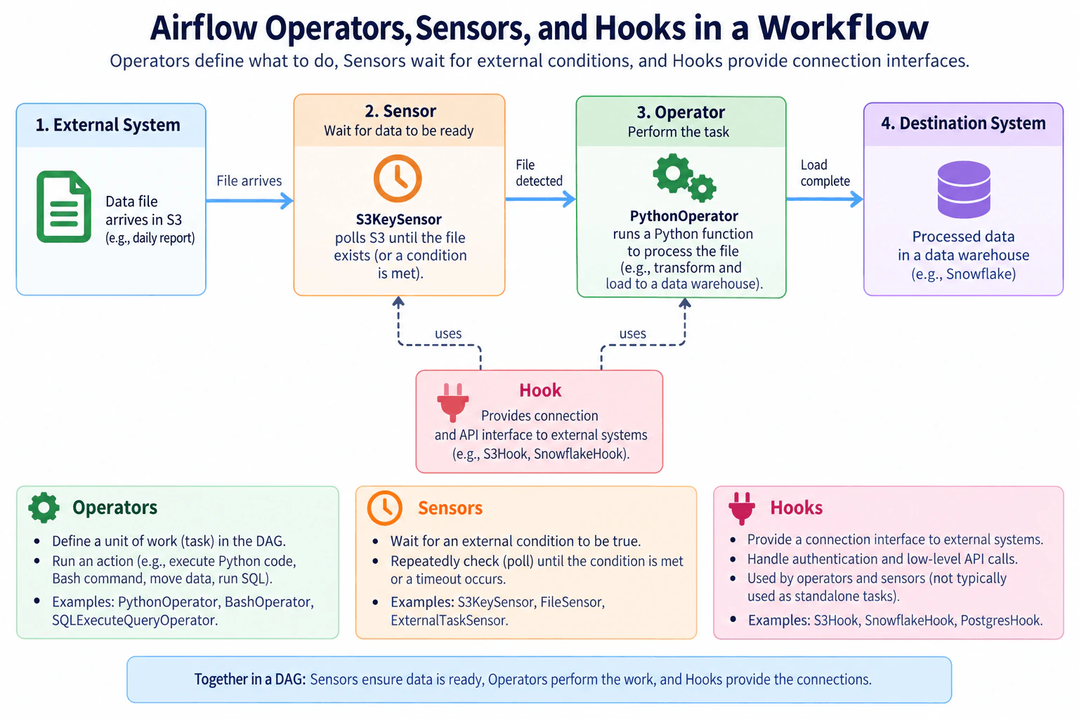
In an Airflow workflow, sensors wait until required data or another external condition is ready, operators perform the actual task, and hooks provide reusable connections to external systems. In the diagram, S3KeySensor waits for a file, PythonOperator processes it, and hooks handle S3 or warehouse access. This separation keeps workflow logic clear. The main trade-off is that polling sensors can consume resources while waiting, depending on how their waiting mode is configured.
Detailed Explanation
The question asks you to explain three different jobs inside one automated workflow. One part waits until something outside the workflow is ready, such as a new file. Another part performs the useful work once it is allowed to continue. A third part provides a reusable way to communicate with outside systems. The important idea is that these responsibilities are separate but work together. In the shown example, a file becomes available, the workflow waits for it, processes it, and then sends the processed result to a destination system.
Useful Questions to Ask the Interviewer
Do you want the distinction at the conceptual level, or should I also explain how these components interact in a DAG?
Should I discuss sensor polling behavior and its resource trade-off?
How to Explain It in an Interview
1. Start with the workflow responsibility
I would first separate the three concepts by responsibility. An operator defines a unit of work in a DAG. A sensor is a specialized task whose purpose is to wait until a condition becomes true. A hook is not normally the business task itself; it is a reusable connection and API interface that code, operators, or sensors use to communicate with external systems.
The diagram shows those responsibilities in one simple flow rather than as unrelated definitions.
2. The sensor controls when processing may continue
The external system in the diagram is S3. A data file arrives there. The S3KeySensor waits until the expected file exists before the downstream processing task can continue.
That makes the sensor part of the orchestration control flow. Its job is not to transform the file. It checks readiness. The visible arrow from the external system to the sensor represents the file becoming available, and the next dependency proceeds after the condition is satisfied.
Sensors can check a condition repeatedly until it succeeds or reaches a configured timeout. The practical trade-off is that frequent polling can create unnecessary work or external API calls, while rescheduling or deferrable waiting can reduce resource usage when supported and configured.
3. The operator performs the actual unit of work
After the sensor condition succeeds, the PythonOperator runs a Python function that processes the file. This is the main work step in the diagram.
Operators define executable tasks in the DAG. Examples shown include PythonOperator, BashOperator, and SQLExecuteQueryOperator. An operator may run Python code, a shell command, or SQL depending on its type.
The key distinction from a sensor is intent: an operator normally performs work, while a sensor primarily waits for a condition before downstream work can proceed.
4. Hooks provide external-system interfaces
The Hook box sits beneath the task flow because hooks support the tasks rather than forming the main sequential workflow shown across the top. The dashed arrows labeled "uses" connect the hook layer to the sensor and operator.
A hook wraps connection and low-level client behavior for an external system. The diagram shows S3Hook, SnowflakeHook, and PostgresHook as examples. This keeps authentication, client creation, and common external-system operations separate from the business logic of the task.
For example, S3KeySensor uses S3-related hook functionality when checking for the file, and task code can use an appropriate hook when communicating with an external destination.
5. Follow the complete diagram flow
The full sequence is: a file arrives in S3, S3KeySensor waits until that file exists, PythonOperator runs the processing function, and the processed result is loaded into the shown data-warehouse destination, illustrated as Snowflake. Hooks provide the reusable external-system connection layer underneath those task interactions.
So a simple interview rule is: sensors answer "is it ready yet?", operators answer "what work should run?", and hooks answer "how does this code communicate with that external system?"
6. Know the important boundary and trade-off
I would emphasize that hooks are connection interfaces, not a replacement for DAG tasks. Operators and sensors appear as task definitions in the workflow, while hooks are generally used by those tasks or by custom code.
The benefit is separation of concerns: waiting logic, processing logic, and external connectivity stay easier to understand and reuse. The downside is that a poorly configured polling sensor may consume unnecessary worker capacity or make excessive external checks, while placing too much low-level connection logic directly inside operators makes tasks harder to maintain.
Technical Approach
Identify whether the component represents a DAG task or a supporting interface.
If it performs a unit of work, classify it as an operator.
If its task is to wait for a condition, classify it as a sensor.
If it provides reusable connectivity or client methods for an external system, classify it as a hook.
Trace the workflow as S3 file arrival -> S3KeySensor readiness check -> PythonOperator processing -> destination, with hooks supporting external-system access.
Practical Insights
The benefit is clear separation of responsibilities. Operators contain work, sensors contain waiting logic, and hooks centralize external-system access. This makes DAGs easier to read and connection code easier to reuse. The downside is that a sensor may repeatedly check an external system while waiting. Frequent polling can create unnecessary requests and may hold execution resources depending on the sensor mode. We accept the sensor pattern when downstream work must not start before an external condition is true, but we should choose an appropriate waiting mode and interval. Hooks reduce duplicated connection code, but they add another abstraction that engineers must understand. The maintenance benefit is that connection handling can be reused without rewriting every task that accesses the external system.
Why Interviewers Ask This
Interviewers ask this because the three concepts are closely related but serve different responsibilities. They want to see whether a candidate can separate workflow control from task execution and external-system connectivity. A strong answer also shows that the candidate understands how these pieces compose inside a DAG instead of treating every Airflow class as the same kind of task.
Common interview mistakes
A common mistake is saying that operators, sensors, and hooks are three equivalent task types. A sensor is a specialized task focused on waiting, while a hook is primarily an interface for external-system connectivity rather than a normal standalone DAG task. Another mistake is saying the sensor processes the arriving data; in this diagram, S3KeySensor only waits for the file and PythonOperator performs the processing. Candidates also sometimes duplicate authentication and low-level client setup directly in every task instead of using the reusable hook and Airflow connection layer.
Interview tip
Use a three-part sentence first: operators do work, sensors wait for conditions, and hooks connect to external systems. Then walk through the diagram from S3KeySensor to PythonOperator and mention that tasks can rely on hooks. Finish by noting the polling-versus-resource trade-off for sensors.
Interviewer may ask next
What would you change if the S3 file sometimes arrives several hours late?
I would keep the same workflow structure but change how the S3KeySensor waits. The requirement that changes is the expected waiting duration and resource efficiency; the PythonOperator and destination remain the same. I would configure a timeout that covers the expected arrival window and choose a waiting behavior that avoids unnecessarily occupying worker resources for hours. The sensor should still be the component that decides when the dependency is satisfied, and PythonOperator should still perform the processing only after that condition succeeds. The S3 connection remains behind Airflow's connection and hook layer, so credentials do not move into task code. If the file never arrives before the timeout, the sensor should fail rather than silently allowing downstream processing to continue. Recovery would involve resolving the missing-source condition and rerunning the appropriate task or workflow according to the DAG's operating policy. The main downside is longer end-to-end completion time, while overly frequent checks can also increase external API traffic.
Why use a hook instead of creating an S3 or warehouse client directly inside every operator or sensor?
I would use the hook because it keeps external-system connection behavior separate from the task's business responsibility. The workflow order does not change: S3KeySensor still waits, PythonOperator still processes, and the destination remains the same. What changes is where connection handling lives. A hook provides reusable client and connection methods, so multiple tasks do not need to duplicate authentication and low-level API setup. Credentials can remain in Airflow's configured connection boundary rather than being embedded in task logic. If an external call fails, the task or sensor using that hook still owns its task state and failure behavior; the hook does not become a separate workflow stage. Validation of the business result also remains the responsibility of the relevant task rather than the hook. The downside is another abstraction layer, and custom connection behavior may require extending or wrapping a hook. The benefit is cleaner tasks, less duplicated client code, and more consistent external-system access.
16. What belongs in an Airflow XCom?Data PipelinesEasy
i Question Details
Discuss task-to-task coordination values and the limits of using XCom to transport bulk datasets.
Short Interview Answer (30-60 seconds)
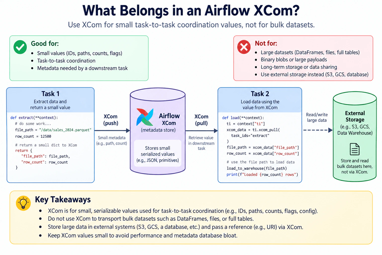
XCom is for small task-to-task coordination values, not bulk datasets. In the diagram, Task 1 returns a file path and row count, XCom carries those small values, and Task 2 pulls them. Task 2 then uses the file path to access the actual data in External Storage such as S3, GCS, or a data warehouse. The key design choice is to pass a reference to large data instead of sending the dataset through XCom.
Detailed Explanation
This question is asking what one step in a workflow should hand to another step. The simple rule is to pass only small pieces of information that help the next step continue its work. Examples are a location, identifier, count, flag, or setting. The first step should not hand over an entire large dataset through this mechanism. In the diagram, Task 1 produces a file location and row count. Task 2 receives those small values and then uses the location to work with the real data stored elsewhere.
Useful Questions to Ask the Interviewer
Are you asking about the normal case where XCom carries small coordination values while the bulk dataset stays in External Storage?
Do you want me to explain why passing a path or URI is better than passing a large DataFrame or file through XCom?
How to Explain It in an Interview
1. Define what belongs in XCom
I would start by saying that XCom is for small task-to-task coordination values. In the approved diagram, suitable values include IDs, paths, counts, flags, configuration values, and other small metadata needed by a downstream task.
Task 1 performs extraction work and returns a small dictionary containing "file_path" and "row_count". These values describe the result of the task without carrying the actual bulk dataset. That keeps the coordination message small and gives Task 2 only the information it needs to continue.
2. Follow the XCom push from Task 1
The diagram shows Task 1 sending small metadata toward Airflow XCom through the arrow labeled "XCom (push)". The example payload contains the file path and row count.
The important point is that the XCom value is metadata about the produced data. It is not the Parquet file itself. The large dataset remains outside the XCom flow.
3. Pull the value in Task 2
Task 2 retrieves the value through the arrow labeled "XCom (pull)". The task reads the "file_path" and "row_count" fields from the XCom result produced by the extract task.
This is the task-to-task coordination flow shown in the diagram: Task 1 produces small metadata, XCom makes that value available, and Task 2 retrieves it. XCom therefore helps one task tell another task what result to use next.
4. Keep bulk data in External Storage
The large-data path is separate. The diagram shows Task 2 reading or writing large data through External Storage, with examples including S3, GCS, and a data warehouse.
Large datasets such as DataFrames, files, full tables, and binary blobs should not be transported through XCom. Instead, store the data in the external system and pass a reference such as a path or URI through XCom. Task 2 then uses that reference to access the real dataset.
5. Explain the trade-off
The benefit is a clear separation of responsibilities. XCom carries small coordination values, while External Storage carries the bulk dataset. This avoids using Airflow's orchestration metadata path as a large-data transport mechanism and helps prevent unnecessary metadata growth.
The downside is that Task 2 must make a separate access to External Storage after pulling the reference. We accept that because the storage system is the appropriate place for large datasets, while XCom remains focused on lightweight communication between tasks.
Technical Approach
Decide whether the value is small coordination metadata or the actual bulk dataset.
Put small values such as IDs, paths, counts, flags, configuration values, or compact metadata in XCom.
Store large DataFrames, files, full tables, and binary payloads in External Storage.
Pass only a reference such as a file path or URI through XCom.
Let the downstream task pull that reference from XCom and use it to access the actual dataset.
Practical Insights
The benefit is that XCom stays lightweight and focused on communication between tasks. A file path, ID, count, or flag is much smaller than a full dataset, so the orchestration metadata path does not have to carry large business data. The downside is that Task 2 must separately access External Storage after it receives the reference. That means the task depends on both the small XCom value and the referenced data being available. We accept this because External Storage is designed to hold large files or tables, while XCom is designed for coordination. The main operational trade-off is therefore one extra storage access in exchange for keeping bulk datasets out of Airflow's task-to-task metadata mechanism.
Why Interviewers Ask This
Interviewers ask this to test whether you understand the boundary between workflow coordination metadata and business data. A strong answer shows that you know what information tasks should exchange through Airflow, why large datasets belong in a separate storage system, and how a downstream task can use a lightweight reference instead. It also tests whether you can explain an important production trade-off without treating XCom as a general-purpose data transport layer.
Common interview mistakes
The main mistake is treating XCom as a general-purpose data transport or long-term storage mechanism. Passing a DataFrame, complete file, full table, or large binary payload through XCom violates the boundary shown in the diagram. Another mistake is storing the bulk data externally but still copying the same large payload into XCom. A better design is to keep the actual dataset in External Storage and pass only the path, URI, ID, count, flag, or other small metadata that the downstream task needs.
Interview tip
Lead with the rule: XCom is for small task-to-task coordination values, not bulk datasets. Then use the diagram's example: Task 1 returns a file path and row count, Task 2 pulls them, and the actual data stays in External Storage. Finish with the memorable phrase: pass references, not datasets.
Interviewer may ask next
What would you change if the extracted dataset became much larger?
I would not change the XCom contract just because the bulk dataset became larger. Task 1 would still return only small coordination metadata such as the file path and row count. XCom would continue to carry those values to Task 2, while the actual dataset would remain in External Storage.
The requirement that changes is the amount of business data, not the purpose of XCom. Task 2 would still pull the same small metadata and then access the large dataset through the external system shown in the diagram. This keeps the task-to-task flow and the large-data flow separate.
For correctness, the XCom value must still point to the intended dataset. The approved diagram does not define a special retry, replay, or recovery mechanism, so I would not invent one. I would keep the same architecture and existing task behavior. The downside is that Task 2 still needs a separate storage access, but that is preferable to moving a larger payload through XCom.
Why pass the file path and row count through XCom instead of passing the Parquet file itself?
I would pass the file path and row count because they are small coordination values, while the Parquet file is the bulk dataset. Task 2 needs to know where the data is and may use the row count as useful metadata, but it does not need the file contents to travel through XCom.
The diagram separates these two flows. Task 1 sends the small metadata into XCom. Task 2 pulls that metadata. Task 2 then reads or writes the large data through External Storage. This keeps Airflow XCom focused on task-to-task coordination and keeps the actual dataset in the system intended to store it.
The main downside is that Task 2 must make a separate access to External Storage. The approved design accepts that trade-off because it avoids using XCom for DataFrames, files, full tables, or large binary payloads. No additional failure or recovery mechanism is shown, so the rest of the original design remains unchanged.
17. Compare dbt’s view, table, incremental, and ephemeral materializations.Data PipelinesEasy
i Question Details
Explain what each materialization creates and how that changes build work and downstream access.
Short Interview Answer (30-60 seconds)
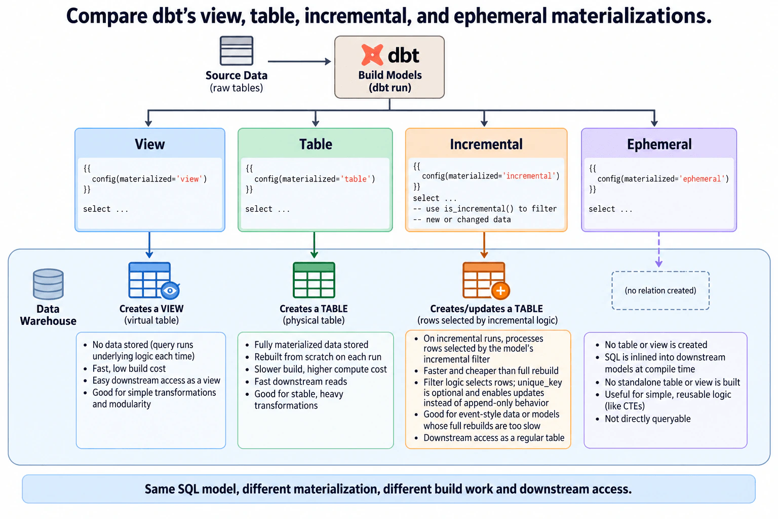
The big picture is that the same dbt model can behave differently depending on its materialization. A view creates a virtual warehouse object with low build work. A table stores the complete result but is rebuilt on a normal run. Incremental also stores a table, but later runs process rows selected by incremental logic. Ephemeral creates no standalone relation; its SQL is inlined into dependent models. The main trade-off is build work versus downstream query work, storage, and direct accessibility.
Detailed Explanation
This question asks how four ways of preparing the same transformed data differ. One option keeps the result as a definition that is evaluated when someone reads it. Another saves the complete result so later reads can use stored data. A third also saves the result but tries to process only the rows selected for the next update. The last option does not create its own saved result at all; its logic becomes part of another model. The practical decision is where the work happens and whether the result must be directly accessible.
Useful Questions to Ask the Interviewer
Should I focus only on what each materialization creates, or also explain when I would choose each one?
Should I assume normal dbt runs rather than a forced full refresh for incremental models?
How to Explain It in an Interview
1. Start with the common dbt model flow
I would start by saying that dbt reads the source relations and builds models during dbt run. The SQL transformation may be similar, but the selected materialization changes what dbt creates in the data warehouse. That choice changes both build-time work and how downstream models or users access the result.
In the diagram, the dbt build path branches into four alternatives: View, Table, Incremental, and Ephemeral. They are materialization choices, not four pipeline stages executed in sequence.
2. View: create a virtual warehouse object
With materialized='view', dbt creates a VIEW. The transformed rows are not persisted as a separate physical result table. Instead, the warehouse keeps the view definition and evaluates its underlying query when the view is read.
The benefit is low build work because dbt mainly creates or replaces the view definition. Downstream models or users can query the view directly. The downside is that repeated reads can repeatedly execute the underlying transformation logic. This is useful for simpler transformations where a separately stored result is unnecessary.
3. Table: materialize the complete result
With materialized='table', dbt creates a physical TABLE containing the model result. On a normal run, dbt rebuilds that materialized result from the model SQL.
Compared with a view, more transformation work happens during the build and the result consumes warehouse storage. The benefit is that downstream reads use the already materialized table rather than reevaluating the complete model query each time. This is a good fit for stable or heavier transformations where storing the result is useful.
4. Incremental: keep a table while reducing later build work
An incremental model also creates a TABLE. The first build creates the table, while later incremental runs process the rows selected by the model’s incremental logic rather than necessarily rebuilding every row.
A model commonly uses is_incremental() to apply a filter only during incremental runs. The important correctness decision is the filter: it must select every row that needs to be processed. A unique_key is optional. When the configured incremental behavior needs to match incoming rows to existing records, the key identifies those records and can support update-style behavior instead of simple append-only loading.
This approach is useful for event-style data or models whose full rebuilds have become too slow. The downside is additional model logic and greater responsibility for choosing the correct rows on every incremental run.
5. Ephemeral: reuse SQL without creating a standalone relation
With materialized='ephemeral', dbt creates no standalone table or view for that model. Instead, dbt inlines the ephemeral model’s SQL into downstream models that reference it, commonly as a common table expression during compilation.
Because there is no independent warehouse relation, the ephemeral model is not directly queryable on its own. Its main value is reusable transformation logic that only exists as part of another dbt model. The transformation work therefore executes as part of the downstream model that contains the inlined logic.
6. Compare the build and access trade-offs
I would finish by comparing where the work happens. View keeps build work low but may shift more work to query time. Table performs the complete transformation during the build and stores the result. Incremental also stores a table but reduces later build work by processing rows selected by incremental logic. Ephemeral stores no standalone result and moves its SQL into dependent models.
So the choice comes down to build cost, query cost, storage, transformation complexity, and whether downstream consumers need a directly queryable warehouse object. The diagram does not define retries, backfills, quality gates, or failure-recovery paths, so I would not invent those behaviors for this question.
Technical Approach
Decide whether the model needs its own directly queryable warehouse relation.
If no standalone relation is needed and the logic is mainly reused by other dbt models, consider ephemeral.
If a relation is required, decide whether the transformed rows should be stored physically.
Use a view when low build work is preferred and query-time evaluation is acceptable.
Use a table when the complete result should be materialized for downstream reads.
Use incremental when the result should remain a table but repeated full rebuilds are too expensive and the model can safely identify the rows that must be processed on later runs.
Practical Insights
The benefit of a view is low build work and no separate physical result table. The downside is that downstream queries may repeatedly execute its underlying transformation logic. The benefit of a table is that downstream readers use an already materialized result, while the downside is the work and storage required to rebuild and store it. Incremental reduces repeated build work because later runs process rows selected by incremental logic. The downside is more correctness logic around which rows must be processed and, when needed, how existing rows are matched. Ephemeral avoids another standalone warehouse relation and is useful for reusable logic. Its downside is that the SQL becomes part of downstream models and cannot be queried independently. We accept these trade-offs according to build cost and downstream access needs.
Why Interviewers Ask This
Interviewers ask this to test whether you understand materialization as an engineering trade-off rather than just configuration syntax. They want to see whether you can connect dbt build work, warehouse storage, downstream query behavior, and model reuse. A strong answer distinguishes a full table rebuild from incremental processing and recognizes that an ephemeral model is compiled into dependent models instead of being exposed as its own warehouse table or view.
Common interview mistakes
Common mistakes are saying that all four materializations create tables, saying an ephemeral model is directly queryable, or describing View, Table, Incremental, and Ephemeral as sequential pipeline stages instead of alternative materializations. Another mistake is saying an incremental model automatically knows which rows are new or changed; the model’s incremental logic must define what to process. It is also incorrect to say that unique_key is always required. It is optional and is relevant when the incremental behavior needs to match incoming rows with existing records.
Interview tip
Compare each materialization using the same three questions: What does dbt create? Where does the transformation work happen? Can downstream users query it directly? Then summarize the trade-off: view means low build work with query-time evaluation; table means a stored full result; incremental means a stored table with selective later processing; ephemeral means reusable SQL with no standalone relation.
Interviewer may ask next
What would you change if the table model became too expensive to rebuild as the dataset grew?
I would consider changing that model from table to incremental while keeping the rest of the shown design unchanged. The changed requirement is build efficiency: instead of rebuilding the complete physical result on each normal run, later incremental runs should process only the rows selected by the model’s incremental logic.
The affected component is the dbt model and its table output. I would add a reliable incremental condition, commonly guarded by is_incremental(), that identifies every row that must be processed. If the chosen incremental behavior needs to match new input with existing records, I would configure an appropriate unique_key for that identity.
Correctness depends on the selection logic not missing required rows. I would compare the incremental result with the expected complete model result during rollout or validation. The diagram does not define a retry or recovery mechanism, so I would not invent one. A complete rebuild remains the conceptual fallback when the table must be reconstructed. The main downside is added model complexity and the risk of incorrect incremental filtering.
When would you choose an ephemeral model instead of a view?
I would choose ephemeral when the transformation is reusable inside other dbt models but does not need to exist as its own directly queryable warehouse relation. The changed requirement is downstream accessibility. A view creates a named VIEW that can be queried directly, while an ephemeral model creates no standalone table or view.
The affected flow is the downstream dbt model that references the ephemeral model. dbt inlines the ephemeral SQL into the dependent model, commonly as a common table expression during compilation. The source data and the other materialization choices remain unchanged.
Correctness still depends on the inlined SQL producing the expected rows when the dependent model runs. There is no separate ephemeral relation to inspect or query independently. The diagram also defines no separate retry, security, or recovery path for it, so those behaviors should not be invented. The main downside is reduced independent visibility and potentially more complex compiled SQL in downstream models.
18. What does a dbt model contain, and what happens when it runs?Data PipelinesEasy
i Question Details
Describe the relationship between a model’s SQL file and the warehouse object created during execution.
Short Interview Answer (30-60 seconds)
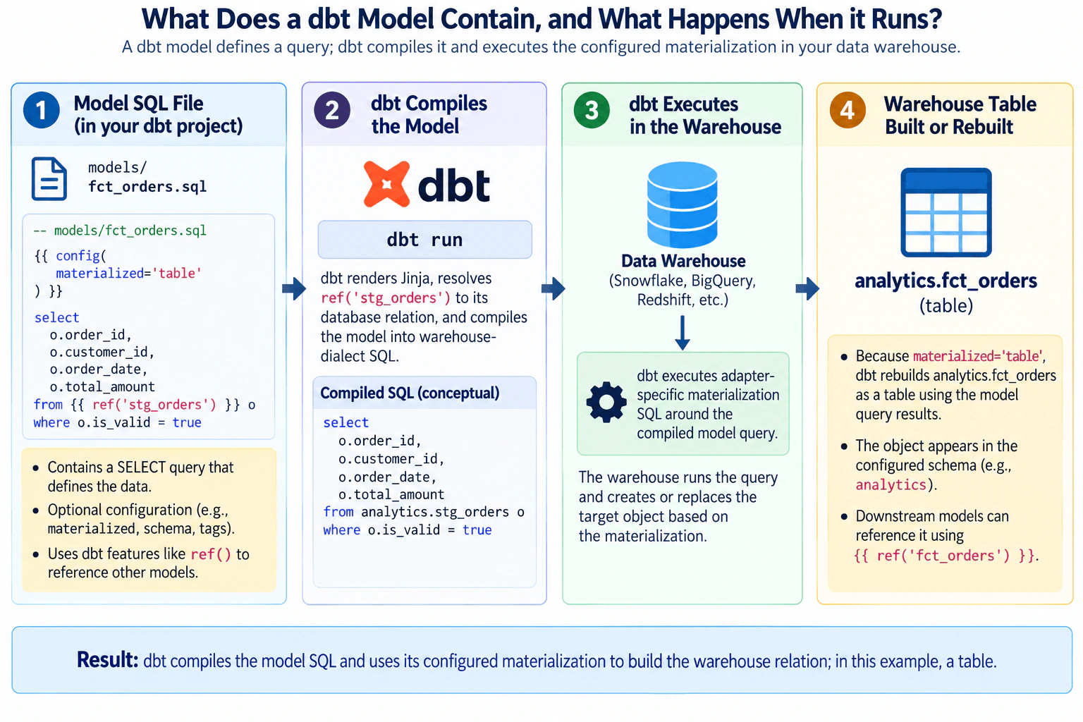
A dbt model is a SQL file containing a SELECT query, optional configuration, and references to other models. During dbt run, dbt renders Jinja, resolves ref(), and compiles warehouse-dialect SQL. The warehouse executes the configured materialization. Here, materialized='table' makes dbt build or rebuild analytics.fct_orders as a table. The benefit is a simple SQL-based transformation model; the trade-off is that physical build behavior depends on the chosen materialization and warehouse adapter.
Detailed Explanation
This question asks how a saved set of instructions becomes a usable result in a data system. The file describes which information should be selected and shaped, and it can also include settings that control how the finished result is stored. When the work starts, the tool reads the file, replaces references with their real locations, prepares instructions that the storage system understands, and sends those instructions there. The storage system performs the work. In this example, the final result is rebuilt as a stored table named analytics.fct_orders.
Useful Questions to Ask the Interviewer
Should I explain the general dbt model lifecycle, or focus on the materialized='table' example shown here?
Do you want me to distinguish the compiled model query from the warehouse-specific materialization SQL?
How to Explain It in an Interview
1. Start with the model SQL file
I would start by saying that the dbt model is the transformation definition, not the finished warehouse table. In the diagram, the model is models/fct_orders.sql. It contains a SELECT query that returns order_id, customer_id, order_date, and total_amount from ref('stg_orders'), with the filter o.is_valid = true. It also has optional configuration. The important setting here is materialized='table'. The model uses ref('stg_orders') instead of hard-coding the upstream warehouse relation, so dbt can resolve that dependency for the active target environment.
2. dbt renders and compiles the model
When dbt run processes this model, dbt handles the dbt-specific parts before warehouse execution. It renders the Jinja expressions, evaluates the config(), and resolves ref('stg_orders') to the corresponding database relation. The diagram shows the resulting conceptual compiled query reading from analytics.stg_orders. The important distinction is that the source file contains dbt-aware SQL and Jinja, while the compiled model contains warehouse-dialect SQL with the reference resolved.
3. The warehouse performs the data processing
The compiled model is executed in the configured data warehouse. The diagram gives Snowflake, BigQuery, and Redshift as examples, but it does not require one particular warehouse. dbt uses its warehouse adapter to submit the required SQL. The warehouse performs the query processing. dbt does not move the business data into a separate processing engine for this flow. The exact SQL used to create or rebuild the target relation can differ by adapter, so I would not claim that every warehouse uses the same CREATE or REPLACE statement.
4. Materialization determines the resulting relation
The model is explicitly configured with materialized='table'. That means dbt uses its table materialization behavior to build or rebuild analytics.fct_orders as a table from the model query results. The adapter-specific materialization SQL wraps or otherwise uses the compiled model query to produce the target relation. This distinction matters because the compiled SELECT describes the data result, while the materialization controls how that result is persisted in the warehouse.
5. Keep the model file and warehouse table separate
The main interview takeaway is that models/fct_orders.sql and analytics.fct_orders are related but are not the same object. The SQL file is the transformation definition. dbt interprets config() and ref(), compiles the query, and coordinates execution through the warehouse adapter. The warehouse executes the work and stores the result. In this example, that result is a table. A downstream dbt model can then use ref('fct_orders') to reference this model without hard-coding analytics.fct_orders.
Technical Approach
Read models/fct_orders.sql and its model configuration.
Identify the SELECT query, including ref('stg_orders') and the o.is_valid = true filter.
Run dbt so it renders Jinja and resolves the model reference.
Compile the model into warehouse-dialect SQL that reads from the resolved relation, shown conceptually as analytics.stg_orders.
Execute the model through the configured warehouse adapter.
Apply the configured table materialization.
Build or rebuild analytics.fct_orders as a table containing the query results.
Allow downstream dbt models to reference the model with ref('fct_orders').
Practical Insights
The benefit is that the transformation stays easy to understand: the developer mainly writes a SELECT query, while dbt handles references, compilation, and materialization. The downside is that building a physical table requires warehouse compute and storage. A table materialization may rebuild a large result when the model runs, which can cost more and take longer than exposing a logical view. The exact physical SQL also depends on the warehouse adapter, so Snowflake, BigQuery, Redshift, or another warehouse may implement the build differently. We accept this because the model definition remains consistent while dbt's adapter handles warehouse-specific details.
Why Interviewers Ask This
Interviewers ask this to see whether a candidate understands the boundary between a dbt model definition and the warehouse relation produced from it. A strong answer distinguishes the SQL written by the developer, dbt's Jinja and ref() compilation, warehouse execution, and materialization behavior. It also shows whether the candidate understands that the SQL file is not itself the warehouse table and that the configured materialization determines how the result is persisted.
Common interview mistakes
Common mistakes are saying that the .sql file itself becomes the table, saying dbt performs the data processing outside the warehouse, or treating ref('stg_orders') as the literal physical relation name. Another mistake is saying that the compiled SELECT always contains one universal CREATE TABLE statement. The diagram separates these responsibilities: dbt renders Jinja and resolves ref(), the warehouse executes the query, and adapter-specific materialization logic builds the final relation. For this example, it is also incorrect to call the final relation a table or view interchangeably because materialized='table' explicitly selects a table.
Interview tip
Explain it as one simple sequence: model SQL file -> dbt rendering and compilation -> warehouse execution -> materialized warehouse relation. Use the materialized='table' example consistently. Emphasize that the SQL file defines the transformation, while analytics.fct_orders is the resulting warehouse table.
Interviewer may ask next
What changes if fct_orders becomes very large and rebuilding the whole table on every run is too expensive?
The requirement changes from always rebuilding a complete table to reducing the amount of warehouse work performed on each run. The affected part is the model's materialization strategy, not the basic relationship between the model file, dbt compilation, and warehouse execution. I would first determine whether another dbt materialization is appropriate for that requirement. The model can still contain SQL, config(), and ref('stg_orders'), and dbt still renders and compiles those elements before the warehouse executes the work.
Correctness becomes more important because processing only changed data requires a reliable rule for identifying those changes. The current diagram does not define a unique key, update timestamp, late-arriving-data policy, or backfill rule, so I would ask for those requirements before proposing a concrete incremental implementation. Validation and recovery would then need to confirm that changed and historical rows are handled correctly. The main downside is complexity: rebuilding the full table is simple to reason about, while processing only part of the data introduces state and additional correctness rules.
What is the difference between ref('stg_orders') in the model file and analytics.stg_orders in the compiled SQL?
ref('stg_orders') is the dbt-level reference written by the model author, while analytics.stg_orders is the resolved database relation shown in the diagram's conceptual compiled SQL. The transformation requirement does not change; this follow-up tests the boundary between the source model definition and the SQL that the warehouse executes.
The affected step is dbt compilation. In models/fct_orders.sql, ref('stg_orders') tells dbt that fct_orders depends on the stg_orders model without hard-coding that model's physical relation name. During dbt run, dbt renders the Jinja expression and resolves the reference for the configured target. The compiled query can therefore read from the resolved warehouse relation. The warehouse then executes that query as part of the configured table materialization and produces analytics.fct_orders. Downstream models can similarly reference this result with ref('fct_orders'). The benefit is environment-aware model references and explicit dbt dependencies. The downside is that understanding the final warehouse SQL may require inspecting dbt's compiled output rather than only the source model file.
19. Which dbt configuration wins when materialization is specified in several places?Data PipelinesEasy
i Question Details
Compare model-local config, properties YAML, and folder-level settings in dbt_project.yml.
Short Interview Answer (30-60 seconds)
The big picture is that dbt uses the most specific setting when the same configuration is defined in several places. Here, the folder-level setting is view, the properties YAML sets the orders model to table, and orders.sql sets incremental with config(). The model-local value has the highest precedence, so orders is materialized as incremental. The benefit is flexible defaults with targeted overrides; the downside is that scattered configuration can be harder to trace.
Detailed Explanation
This question asks how one final choice is made when the same option is written in three places. One place sets a broad default for a folder, another sets a value for one named item, and the last writes a value directly inside that item. When these choices disagree, the value closest to the individual item takes priority. In the attached example, the three choices are view, table, and incremental. The value written directly in the individual file is incremental, so that becomes the final choice.
Useful Questions to Ask the Interviewer
Should I compare only the three locations shown: model-local config, properties YAML, and folder-level dbt_project.yml?
Do you want only the precedence rule, or should I also explain how I would troubleshoot an unexpected effective materialization?
How to Explain It in an Interview
1. State the precedence rule
I would start by saying that dbt applies configuration hierarchically, and the most specific value wins when the same configuration is defined at multiple levels. For the three locations in this diagram, the order from highest to lowest precedence is model-local config(), properties YAML for the specific model, and folder-level configuration in dbt_project.yml. The configuration being resolved here is materialized, so dbt needs one effective materialization for the orders model.
2. Read the folder-level default
The broadest setting shown is in dbt_project.yml. Under the marts path, +materialized is set to view. This is the lowest-precedence value among the three locations in the diagram. It works well as a shared default because multiple models under that path can inherit it. However, it does not force orders to remain a view when a more specific materialized value is defined for that model.
3. Apply the properties YAML override
The next level is the properties YAML file, shown as models/marts/schema.yml. It identifies the orders model and sets config.materialized to table. Because this setting targets the specific model, it is more specific than the folder-level view setting. Therefore, table overrides view. If orders.sql did not contain its own materialized configuration, table would be the effective materialization in this example.
4. Apply the model-local configuration
The highest-precedence value is inside models/marts/orders.sql: {{ config(materialized='incremental') }}. This setting is defined directly on the model, so it overrides both table from the properties YAML and view from dbt_project.yml. The final effective materialization is incremental. The key point is that this result comes from configuration specificity, not from assuming that whichever file is read last wins.
5. Explain the practical trade-off
The benefit is that teams can set broad defaults and override only the exceptions. A folder can default to views while one model uses a table or incremental materialization. The downside is discoverability: when configuration is spread across several files, a developer may need to trace multiple locations to understand the effective value. For this materialized setting, the more specific value replaces the less specific value rather than combining with it.
6. Finish with the exact diagram result
For this diagram, there are three conflicting materialization values for orders: view at the folder level, table in the properties YAML, and incremental in orders.sql. Model-local config() has the highest precedence, so orders is materialized as incremental. A concise interview summary is: model-local config() overrides properties YAML, and properties YAML overrides the applicable folder-level dbt_project.yml setting.
Technical Approach
Identify every location that defines the same configuration key, here materialized.
Match each value to its scope: folder-level dbt_project.yml, model-specific properties YAML, or model-local config().
Rank those locations by specificity.
Select the most specific value that is present instead of relying on file load order.
In the diagram, incremental in orders.sql wins over table in schema.yml and view in dbt_project.yml.
Practical Insights
There is no meaningful algorithmic time or memory complexity in this question. The important cost is maintenance complexity. The benefit is that a team can define a broad default once and override only models that need different behavior. The downside is that the effective value can be harder to discover when configuration is spread across dbt_project.yml, properties YAML, and the SQL model. We accept this because hierarchical configuration reduces repetition while still allowing precise exceptions. A practical approach is to keep broad defaults simple, use model-specific overrides intentionally, and trace from the most specific configuration outward when a model uses an unexpected materialization.
Why Interviewers Ask This
Interviewers ask this to see whether you understand configuration inheritance instead of only memorizing dbt syntax. A Data Engineer should know where a model can receive configuration, which value overrides another, and how to diagnose an unexpected build result. The question also tests whether you can explain precedence clearly and distinguish a model-specific override from a broader folder default without introducing unrelated pipeline behavior.
Common interview mistakes
A common mistake is saying that dbt_project.yml always wins because it is the main project file. Another is treating properties YAML and model-local config() as equal precedence. Candidates may also describe the result as dependent on file-loading order, which misses the actual rule: configuration specificity determines the winner. In this diagram, another mistake is stopping at table because schema.yml overrides the folder-level view while forgetting that orders.sql contains the still more specific incremental setting.
Interview tip
State the precedence order immediately: model-local config() > properties YAML > folder-level dbt_project.yml. Then walk through the three values in the diagram and finish with the effective result, incremental. This shows both the rule and how to apply it.
Interviewer may ask next
What happens if the model-local materialized='incremental' configuration is removed from orders.sql?
The properties YAML value becomes the winner, so orders would be materialized as a table in this example. The requirement changes because the highest-precedence configuration is no longer present. I would compare the two remaining values: schema.yml sets materialized to table for the specific orders model, while dbt_project.yml sets the broader marts path to view. The model-specific properties YAML is more specific, so table overrides the folder-level default. Nothing else about the precedence rule changes. There is no retry, replay, or recovery path involved because this is configuration resolution rather than a runtime pipeline failure. To validate the change, I would confirm that orders.sql no longer sets materialized and then inspect the model's properties YAML and applicable project-level path. The main downside remains maintainability: the effective value may still require checking more than one file. The unchanged rule is that the most specific available configuration wins.
What happens if both the model-local config and the properties YAML materialization are removed?
The applicable folder-level dbt_project.yml value becomes effective, so orders would use view in the diagram's example. The requirement changes because both more-specific overrides have been removed. The only materialized value shown for the model is then the marts path setting, +materialized: view, so orders inherits that broader default. Correctness still comes from the same specificity rule; there is simply no higher-precedence value left to replace it. I would validate the result by confirming that orders.sql has no materialized config() value and that the properties YAML entry for orders has no materialized setting. No separate recovery process is needed because no execution failure occurred. The benefit is simpler configuration with fewer overrides. The downside is reduced model-specific control if orders later needs a different materialization from the other models that inherit the same folder-level setting.
20. How does Airflow’s TaskFlow interface differ from classic operator-based authoring?Data PipelinesMedium
i Question Details
Address dependency inference, function outputs, and interoperability with existing operators.
Short Interview Answer (30-60 seconds)
Both styles can express the same workflow. Classic Airflow usually creates operator objects and wires dependencies explicitly with >> or <<. TaskFlow uses @task-decorated Python functions, infers dependencies when one task's output is passed to another, and represents returned values through XCom-backed outputs. The benefit is less boilerplate and clearer Python data flow. The trade-off is that existing operators are still useful, so production DAGs often mix both styles.
This question asks about two ways to describe the same sequence of work. In the older style, you create a separate object for each step and then state which step must happen before another. In the newer style, you write normal-looking functions and connect them by passing one result into the next. The system can then understand both the order of work and the value being passed. The main idea is not that one method replaces the other. They can be combined when that makes the workflow easier to understand and maintain.
Useful Questions to Ask the Interviewer
Should I focus only on authoring style, or also explain how task outputs move between steps?
Would you like me to include how TaskFlow tasks work with existing operators in the same DAG?
How to Explain It in an Interview
1. Classic authoring is explicit
I would start by saying that classic operator-based authoring creates Airflow operator objects directly. In the diagram, extract is a BashOperator, transform is a PythonOperator, and load is another BashOperator. Their order is declared explicitly as extract >> transform >> load.
That style is very readable when each step already maps naturally to an Airflow operator. The author creates the tasks first and then declares their upstream and downstream relationships. Assuming the Airflow 3.x public authoring interface shown in the diagram, those standard operators come from the standard provider package.
2. TaskFlow uses decorated Python functions
TaskFlow is a more Pythonic authoring interface. A normal Python function is decorated with @task. When that decorated function is called while the DAG is being defined, Airflow creates a task representation instead of immediately running the function body.
The diagram shows extract(), transform(input_path), and load(clean_path) as TaskFlow tasks. This removes much of the boilerplate required to construct PythonOperator objects for ordinary Python logic.
3. TaskFlow can infer dependencies from outputs
The biggest difference is dependency inference. Classic tasks commonly use explicit relationships such as >> or <<. TaskFlow can derive a dependency when a downstream task consumes an upstream task's output.
In the diagram, load(transform(extract())) means transform depends on extract, and load depends on transform. Airflow knows this because each decorated task call returns an object representing that task's result rather than the final runtime Python value.
4. Returned values become XCom-backed task outputs
TaskFlow also makes small outputs easier to use. The diagram's extract task returns /tmp/data.csv, and transform receives that output as input_path. Transform returns /tmp/cleaned.csv, which becomes the input to load.
These values are represented through Airflow's XCom mechanism. They are not passed directly from one worker's memory to another worker. Classic operators can also expose XCom-backed outputs, so XCom is not unique to TaskFlow. TaskFlow mainly makes the authoring experience more natural because ordinary function return values can be used as downstream task inputs.
5. TaskFlow and classic operators can be mixed
The two styles are interoperable. The diagram's mixed example uses a TaskFlow extract task, a classic BashOperator named transform, and a TaskFlow load task. The explicit raw >> transform relationship places the operator after extract. Then load(transform.output) passes the operator's XCom-backed output into the downstream TaskFlow task.
So I would not describe TaskFlow as a replacement for every operator. I would use TaskFlow for Python-centric logic and existing operators when they already provide a clear abstraction. The benefit is cleaner Python code; the downside is that a mixed DAG uses two authoring styles, so task naming and dependencies should stay simple.
Key Insight / Why This Solution Works
Identify which steps are plain Python logic and which steps already map well to existing Airflow operators.
For classic authoring, instantiate the operators and declare their dependencies explicitly.
For Python-centric steps, use @task-decorated functions.
Pass an upstream TaskFlow output into a downstream TaskFlow call when the downstream task needs that value; this lets Airflow infer the dependency and represent the value through XCom.
When mixing styles, connect TaskFlow tasks and operators with explicit dependencies or output objects as appropriate.
Use XCom-backed outputs for small coordination values rather than treating orchestration metadata as bulk-data transport.
Code
from datetime import datetime
from airflow.sdk import DAG, task
from airflow.providers.standard.operators.bash import BashOperator
from airflow.providers.standard.operators.python import PythonOperator
# Classic authoring: create operator tasks and wire their order explicitly.with DAG(
dag_id="classic_dag",
start_date=datetime(2024, 1, 1),
schedule="@daily",
catchup=False,
) as classic_dag:
extract = BashOperator(
task_id="extract",
bash_command="echo 'Extracting data'",
)
# PythonOperator wraps this Python callable as an Airflow task.
transform = PythonOperator(
task_id="transform",
python_callable=lambda: print("Transforming data"),
)
load = BashOperator(
task_id="load",
bash_command="echo 'Loading to warehouse'",
)
# The classic dependency chain is declared explicitly.
extract >> transform >> load
# TaskFlow authoring: task-output usage expresses data flow and dependencies.with DAG(
dag_id="taskflow_dag",
start_date=datetime(2024, 1, 1),
schedule="@daily",
catchup=False,
) as taskflow_dag:
@taskdefextract_data() -> str:
# The return value becomes an XCom-backed task output.return"/tmp/data.csv" @taskdeftransform_data(input_path: str) -> str:
# Airflow resolves the upstream task output when this task runs.print(f"Transforming {input_path}")
return"/tmp/cleaned.csv" @taskdefload_data(clean_path: str) -> None:
# This task depends on transform because it consumes transform's output.print(f"Loading {clean_path} to warehouse")
load_data(transform_data(extract_data()))
# Interoperability: TaskFlow tasks and classic operators can share one DAG.with DAG(
dag_id="mixed_dag",
start_date=datetime(2024, 1, 1),
schedule="@daily",
catchup=False,
) as mixed_dag:
@taskdefmixed_extract() -> str:
# Return a small coordination value rather than a large dataset.return"raw"
transform_op = BashOperator(
task_id="transform",
bash_command="echo transformed",
)
@taskdefmixed_load(result: str) -> None:
# The TaskFlow task receives the operator's XCom-backed output.print(result)
raw = mixed_extract()
# Explicitly place the existing operator downstream of extract.
raw >> transform_op
# Passing operator.output establishes the downstream data relationship.
mixed_load(transform_op.output)
Why Interviewers Ask This
Interviewers ask this to check whether you understand Airflow's authoring model rather than only its syntax. They want you to separate dependency wiring from data passing, explain why TaskFlow return values become XCom-backed outputs, and understand that existing operators still work with TaskFlow. A strong answer also shows practical judgment about when cleaner Python functions are useful and when a purpose-built operator remains the clearer choice.
Common interview mistakes
A common mistake is saying TaskFlow is a different execution engine or that it replaces all operators. It is an authoring interface, and existing operators can still be used. Another mistake is saying only TaskFlow uses XCom; classic operators can also expose XCom-backed outputs. Do not say TaskFlow return values move directly between worker memory spaces. Airflow represents those results through its task-output/XCom mechanism. Also avoid saying every dependency is automatically inferred. Classic relationships may remain explicit, and mixed DAGs often use both explicit dependency wiring and output-based relationships.
Interview tip
Structure the answer around the three things the question asks: dependency inference, function outputs, and interoperability. Contrast extract >> transform >> load with load(transform(extract())), explain that TaskFlow returns are XCom-backed outputs, and finish by showing that an existing operator can sit between TaskFlow tasks. That demonstrates both the syntax difference and the practical production trade-off.
Interviewer may ask next
What would you change if a TaskFlow task needed to produce a very large dataset instead of a small path or identifier?
I would keep the DAG structure but stop returning the large dataset itself through TaskFlow. The changed requirement is the size of the data crossing the task boundary. XCom-backed task outputs are useful for coordination values, but Airflow's orchestration metadata should not become the bulk-data transport layer. I would have the producing task write the large result to the workflow's proper external data location and return only a small reference, such as a path or identifier. The downstream task would receive that reference through the same TaskFlow dependency mechanism and read the actual data from that location. The dependency graph therefore stays the same. For failure handling, the producing task must not return the reference until the intended output is available, and the consumer should fail clearly if the referenced data cannot be read. A retry can then reuse or recreate the external output according to the task contract. The downside is additional lifecycle and cleanup responsibility for externally stored intermediate data.
How would you add an existing classic operator to a DAG that otherwise uses TaskFlow?
I would keep the TaskFlow tasks that already express the Python logic clearly and insert the existing operator only for the step it represents well. The requirement changes only at that task boundary, not for the whole DAG. If a TaskFlow task must complete before the operator, I can declare that relationship explicitly, as the diagram does with raw >> transform_op. If a downstream TaskFlow task needs the operator's result, I can pass transform_op.output into that decorated task. Airflow then has an XCom-backed result reference and the required downstream relationship. The rest of the TaskFlow flow does not need to be rewritten. Correctness still depends on normal Airflow task state: the downstream task should not successfully consume a required result before its upstream operator succeeds. Recovery remains task-oriented rather than creating a separate pipeline. The main downside is readability: a mixed DAG uses two authoring styles, so I would keep names and dependencies straightforward.
More questions load as you scroll
Disclaimer: This interview guide is for educational and informational purposes only. It is designed to help readers prepare, but it does not guarantee any interview result, hiring decision, offer, or outcome. Interview questions, hiring criteria, and preferred answers can vary by employer, interviewer, industry, location, and time. All answers, examples, and explanations in this guide are suggested examples for interview preparation, not definitive answers or instructions for professional practice. They are based on research and judgment, are provided without warranties of any kind, and should be adapted to the question, role, and applicable laws and professional requirements. Diagrams are simplified illustrations intended to highlight the main concepts and their relationships; actual situations, systems, and practices may be more complex. Alternative approaches may be equally valid or better suited to a particular question, context, or interviewer. To the fullest extent permitted by applicable law, the contributors and publisher are not liable for decisions made, actions taken, or losses incurred based on this guide.
State Laws and Professional Responsibilities: Laws and requirements governing an occupation vary by state and jurisdiction. You are responsible for checking the current laws, licensing requirements, and scope-of-practice rules that apply to your location and role, and for ensuring that your answers and actions comply with them. Adapt examples in this guide to those requirements. This guide is not legal advice.
Content Accuracy and Verification: To the fullest extent permitted by applicable law, we do not represent or warrant that interview guides, questions, answers, examples, or diagrams are accurate, complete, current, error-free, or suitable for any particular purpose. You are responsible for independently reviewing and verifying the information before relying on it.