This interview guide is for educational and informational purposes only. It is designed to help readers prepare, but it does not guarantee any interview result, hiring decision, offer, or outcome. Interview questions, hiring criteria, and preferred answers can vary by employer, interviewer, industry, location, and time. All answers, examples, and explanations in this guide are suggested examples for interview preparation, not definitive answers or instructions for professional practice. They are based on research and judgment, are provided without warranties of any kind, and should be adapted to the question, role, and applicable laws and professional requirements. Diagrams are simplified illustrations intended to highlight the main concepts and their relationships; actual situations, systems, and practices may be more complex. Alternative approaches may be equally valid or better suited to a particular question, context, or interviewer. To the fullest extent permitted by applicable law, the contributors and publisher are not liable for decisions made, actions taken, or losses incurred based on this guide.
State Laws and Professional Responsibilities
Laws and requirements governing an occupation vary by state and jurisdiction. You are responsible for checking the current laws, licensing requirements, and scope-of-practice rules that apply to your location and role, and for ensuring that your answers and actions comply with them. Adapt examples in this guide to those requirements. This guide is not legal advice.
Identity, Image, and Privacy Notice
To respect individual privacy, some names, profile photographs, avatars, biographical details, and other identifying information displayed in this guide may be replaced with pseudonyms, licensed stock images, illustrative avatars, composite images, or representative descriptions. Unless a person is expressly identified as an actual contributor, a displayed name, image, or profile should not be understood as depicting or identifying a specific candidate, interviewer, employee, or other real individual. These representations are provided for editorial and illustrative purposes only and do not imply endorsement, employment, participation, or affiliation with this guide or any company mentioned in it. Any resemblance to an actual person is coincidental.
Company Notice
This guide is an independent educational resource and is not affiliated with, endorsed by, sponsored by, or approved by the company named in this guide. Company names identify reported interview experiences or the employer context of clearly labeled original practice exercises. Interview practices can change without notice, and inclusion of company-specific content does not mean these questions are official, complete, or guaranteed to be asked. To the fullest extent permitted by law, the author, contributors, and publisher are not responsible for outcomes related to use of this material.
Content Accuracy and Verification
To the fullest extent permitted by applicable law, we do not represent or warrant that interview guides, questions, answers, examples, or diagrams are accurate, complete, current, error-free, or suitable for any particular purpose. You are responsible for independently reviewing and verifying the information before relying on it.
Questions or comments?
Contact us for general questions, or share feedback, technical corrections, and comments with the community.
41. When would you use Snowpark for transformations?Cloud Data PlatformsMedium
i Question Details
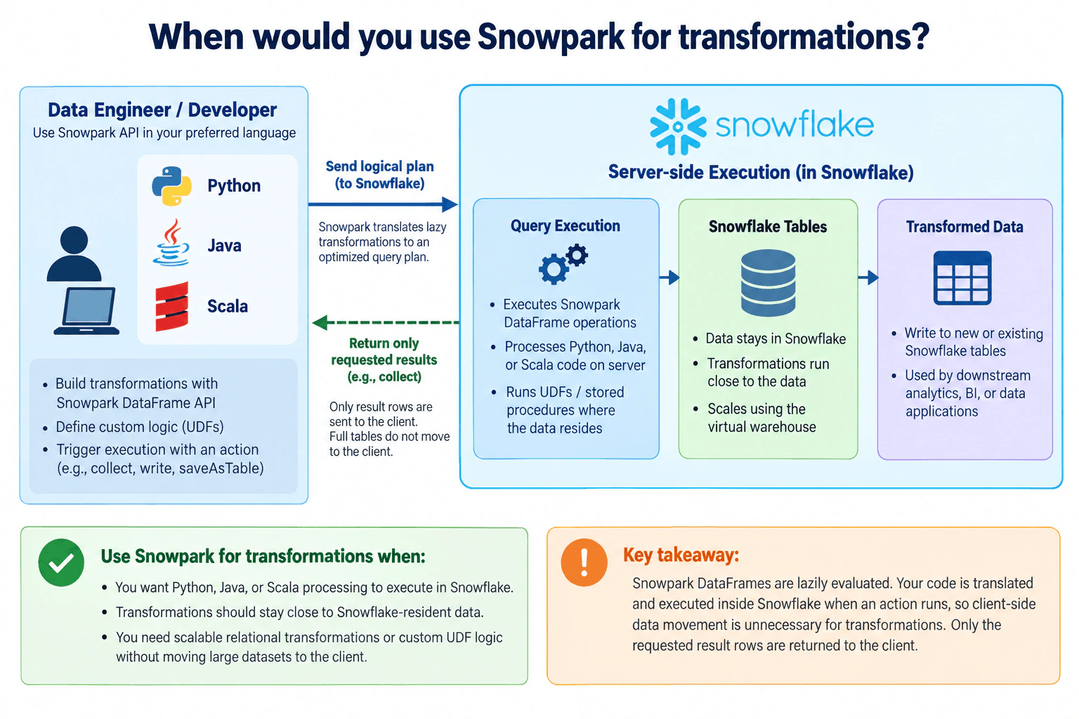
Explain where Python, Java, or Scala processing executes and when client-side data movement is unnecessary.
Short Interview Answer (30-60 seconds)
I would use Snowpark when data already resides in Snowflake and I want Python, Java, or Scala transformations to execute close to that data. Snowpark sends the transformation work to Snowflake instead of moving whole datasets to the client, while requested results can still be returned when needed.
Detailed Explanation
Snowpark is useful for data engineers who prefer Python, Java, or Scala but want warehouse-scale transformations to stay inside Snowflake. Instead of downloading Snowflake tables into an application, transforming them locally, and uploading the result again, the developer builds transformations through the Snowpark API. Snowpark DataFrame operations are lazy, so the transformation is not executed until an action requires a result. Snowflake then executes the generated work against data stored in Snowflake. This design prioritizes data locality, avoids unnecessary movement of large datasets, and still allows requested result rows to return to the client.
Useful Questions to Ask the Interviewer
Does the source data already live primarily in Snowflake, or would the transformation depend heavily on external data?
Are the transformations mainly DataFrame operations such as filtering, joining, grouping, and aggregation, or do they also require supported UDF or stored-procedure logic?
Should the transformed result remain in Snowflake for downstream analytics and applications, or must result rows be returned to a client application?
Is avoiding large client-side data transfers an important requirement for this workload?
How to Explain It in an Interview
Use the Snowpark API from the developer environment The data engineer or developer writes transformation logic with Snowpark in Python, Java, or Scala. The application defines the operations, but normal Snowpark DataFrame processing does not require the complete source tables to be downloaded into client memory. This separates the development environment from the server-side data-processing boundary.
Build transformations lazily Snowpark DataFrame transformations are lazily evaluated. Operations such as filters, joins, projections, grouping, and aggregations describe the transformation without immediately returning all data to the client. When an action requires execution, Snowpark submits the work to Snowflake for processing. This is why a sequence of DataFrame transformations can remain close to the stored data instead of becoming a client-side ETL flow.
Execute the data work inside Snowflake Snowflake executes the transformation using Snowflake compute against Snowflake tables. The large source dataset stays in Snowflake while the query execution layer performs the requested operations. Supported UDFs and stored procedures can also run custom logic in Snowflake when they are part of the transformation design. The important distinction is that the Snowpark client API defines the work, while the supported data-processing work executes on the Snowflake side.
Keep transformed output in Snowflake when possible When the transformation writes a new or existing Snowflake table, the output remains inside Snowflake. That result can then be consumed by downstream analytics, BI workloads, or data applications without a client application becoming an unnecessary bulk-data transfer point.
Return only explicitly requested results to the client The return path is different from the transformation path. An action such as collect intentionally returns result rows to the client. That does not mean the full source tables had to be downloaded before the transformation. If the output is large and another Snowflake-based consumer needs it, writing the result to a Snowflake table is usually a better fit than collecting the entire result into client memory.
Choose Snowpark when data locality matters Snowpark is a strong fit when the source data already resides in Snowflake, the team wants to use Python, Java, or Scala APIs, and the required transformations can execute through Snowflake-supported operations. This includes scalable relational transformations and supported custom UDF logic. Keeping computation near the data avoids unnecessary network movement and reduces dependence on the memory and compute capacity of a developer machine or application host.
Understand the main trade-off The advantage is data locality and use of Snowflake compute instead of moving warehouse-scale datasets to a client. The trade-off is that the transformation workload consumes Snowflake compute and follows Snowflake's execution model. If essential processing must happen in an external runtime that Snowflake cannot execute, then client-side or external processing may be more appropriate even though it introduces additional data movement and operational complexity.
Handle failures at the execution boundary If submission or execution fails, the intended transformation does not successfully produce its result. The client or operator should inspect the Snowflake execution error, correct the cause, and rerun the operation where appropriate. If collect fails, the requested rows are not successfully returned to the client. Recovery is therefore centered on the Snowflake operation rather than replaying an unnecessary bulk download-transform-upload cycle.
Scale with Snowflake compute, not the client machine The transformation workload runs on Snowflake compute, including the virtual warehouse used for the workload. Larger or more concurrent transformations therefore consume more Snowflake compute. Keeping the data server-side reduces unnecessary network movement, but it does not eliminate compute cost. Collecting a large result can still create network and client-memory pressure.
Technical Approach
Confirm that the primary source data resides in Snowflake.
Express the transformation with the Snowpark DataFrame API in Python, Java, or Scala.
Build the transformation lazily so intermediate source tables are not copied to the client.
Trigger execution with an action or table-write operation.
Let Snowflake execute the transformation using Snowflake compute against Snowflake tables.
Keep the transformed output in Snowflake when downstream consumers can use it there.
Return only explicitly requested result rows to the client, such as through collect.
If execution fails, diagnose the Snowflake operation and rerun only after addressing the cause.
Practical Insights
The main scaling boundary is Snowflake compute rather than the client machine. Large transformations can process Snowflake-resident tables without first transferring those tables over the network into Python, Java, or Scala client memory. A collect action still transfers the requested result rows, so a very large collected result can create network and client-memory pressure. Writing results back to Snowflake avoids that return transfer. More complex transformations and higher concurrency consume more virtual-warehouse compute, so data locality reduces unnecessary movement but does not remove compute cost.
Why Interviewers Ask This
Interviewers want to see whether you understand Snowpark's execution boundary instead of treating it like a normal client-side dataframe library. The key judgment is recognizing when transformation work should execute inside Snowflake, close to Snowflake-resident data, so large datasets do not need to move to an external application just to be processed.
Common interview mistakes
A common mistake is saying that Snowpark downloads Snowflake tables into a Python, Java, or Scala process and performs the main transformation locally. Another is claiming that lazy evaluation means data can never return to the client; actions such as collect intentionally return requested rows. It is also inaccurate to say that every arbitrary line of Python, Java, or Scala client code automatically executes inside Snowflake. The Snowpark client defines the operations, while supported DataFrame work and registered server-side logic such as UDFs or stored procedures execute in Snowflake. Finally, avoiding client-side movement does not mean avoiding compute cost because the transformation still consumes Snowflake compute resources.
Interview tip
Anchor the answer on the execution boundary: Snowpark lets you express transformations in Python, Java, or Scala while the supported data-processing work executes inside Snowflake. Then explain lazy DataFrames, server-side execution, keeping output in Snowflake, and the special case where collect deliberately returns requested rows to the client.
Interviewer may ask next
What changes if the application calls collect on a very large Snowpark DataFrame?
The transformation can still execute inside Snowflake, but collect asks Snowpark to return the resulting rows to the client. If that result is large, network transfer and client memory can become important constraints. I would avoid collecting warehouse-scale results when the next consumer can read them directly from Snowflake. Instead, I would write the transformed result to a Snowflake table and let downstream analytics, BI, or data applications consume it there.
When might you choose client-side processing instead of Snowpark for this workload?
I would choose client-side or external processing when the essential computation depends on a runtime or capability that cannot execute through the Snowpark and Snowflake server-side execution model. That changes the architecture because some data may need to leave Snowflake. The trade-off is additional network movement, external compute and memory requirements, and another runtime to operate. When the data already resides in Snowflake and the required transformation is supported there, Snowpark is the cleaner fit because it keeps the heavy data processing close to the data.
42. What role do Snowpark Container Services play?Cloud Data PlatformsMedium
i Question Details
Describe deployment of containerized applications and custom processing alongside data held in Snowflake.
Short Interview Answer (30-60 seconds)
Snowpark Container Services let data teams deploy OCI-based applications and custom processing inside Snowflake on managed compute pools, close to Snowflake data. The main trade-off is gaining custom-runtime flexibility and integrated governance while adding container, compute-pool, and application lifecycle operations beside normal warehouse-based SQL processing.
Detailed Explanation
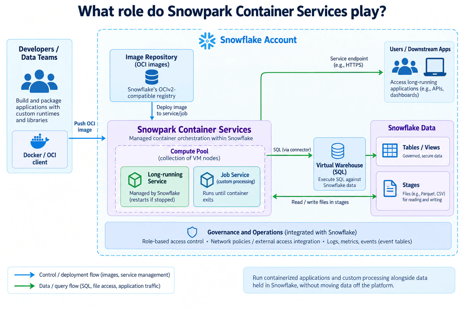
Data teams sometimes need custom runtimes, libraries, APIs, or long-running processes that do not fit normal SQL execution. Moving Snowflake data to a separate application platform would add another network, security, and operating boundary. Snowpark Container Services solve that recurring problem by running containerized services and jobs inside the Snowflake account, while tables, views, stages, and virtual warehouses remain the data and SQL layer. The design prioritizes custom processing close to the data, while keeping image deployment, container compute, SQL execution, file access, serving, governance, and operational evidence as clear responsibilities.
Useful Questions to Ask the Interviewer
Are the workloads mainly long-running APIs or dashboards, finite custom-processing jobs, or a mix?
Will containers mostly query tables through SQL, read and write files in stages, or need both access patterns?
Do any long-running services need an HTTPS endpoint for users or downstream applications?
How much compute isolation is needed between different services and jobs?
Which operational signals matter most for support: service status, job completion, logs, metrics, events, or resource pressure?
How to Explain It in an Interview
Snowpark Container Services extend Snowflake beyond warehouse SQL The main role is to run application code that needs its own containerized runtime while keeping that processing next to data already held in Snowflake. Developers and data teams build the application and its dependencies as an OCI image. Snowpark Container Services then run that image as either a long-running service or a finite job service. This provides a reusable application-compute layer without replacing Snowflake tables, views, stages, or SQL warehouses.
Developers own the application package; Snowflake supplies the managed runtime The developer or data team builds the container image and pushes it from a Docker or other OCI client into the Snowflake image repository. Snowflake's image registry service supports the OCIv2 API for storing OCI-compliant images. This push is a control and deployment flow, not a production-data flow. When a service or job is created, Snowflake uses the chosen image to start the application containers.
Compute pools are the container execution boundary Services and job services run on a compute pool, which is a collection of one or more virtual-machine nodes. A long-running service stays active until explicitly stopped. If one of its containers exits, Snowflake restarts that container. A job service has a finite lifetime and finishes when all of its containers exit; Snowflake does not restart job-service containers simply because they exit. This distinction matters because an API availability failure and a failed processing job require different operational responses.
Container compute does not replace virtual-warehouse SQL compute When application code needs to run SQL against Snowflake data, the container connects to Snowflake and the virtual warehouse executes that SQL against tables or views. The container owns the custom application logic, while the warehouse owns SQL execution. This separation lets each compute system do the work it is designed for, but it also means operators must observe both compute-pool capacity and warehouse behavior.
Containers can work with Snowflake-held files as well as tables The other data path in the diagram is stage access. A service can use a Snowflake internal stage as a mounted stage volume when configured for that purpose, letting the container read and, with the required privileges, write stage files. This is useful for file-oriented custom processing such as Parquet or CSV workloads. Stage-volume behavior is not identical to a general POSIX file system, so applications must respect the supported file-access semantics.
Long-running services can serve downstream users and applications A long-running service can expose a declared service endpoint. When the endpoint is configured for public access, authorized users in the Snowflake account can reach it from outside Snowflake, with HTTP or HTTPS serving supported through the Snowflake service boundary. This makes the pattern suitable for APIs, dashboards, and other applications that need a continuously available process. Endpoint traffic is a data or application-traffic flow and is separate from image deployment.
Governance and operations stay integrated with Snowflake The diagram places role-based access control, network controls, and logs, metrics, and events under the Snowflake governance and operations boundary. Roles and service permissions control who can create or use services and which Snowflake objects workloads can access. Public endpoint access is authenticated and authorized. External Access Integrations govern approved outbound access from services to external destinations when such egress is needed. Logs, metrics, events, and service status provide evidence for deployment, restart, resource, and application failures.
Failures should be handled at the boundary that failed An image or service configuration problem can prevent deployment. A long-running container exit is handled by Snowflake restarting that container, while a job ends when its containers exit and its result must be checked before another execution. SQL failures remain at the virtual-warehouse or query boundary. Stage access can fail because of missing privileges or unsupported file operations. Endpoint problems affect the serving path. Operators should use service status, logs, metrics, events, and returned SQL or file errors to identify the failed boundary before retrying or redeploying.
Scale, cost, adoption, and trade-offs Container workloads consume compute-pool resources, while SQL issued by those workloads consumes virtual-warehouse resources. Long-running services can hold compute-pool capacity over time, while job services consume it during their executions. The practical bottleneck therefore depends on whether the application is container-heavy, SQL-heavy, or file-I/O-heavy. Teams can adopt the pattern workload by workload: containerize only processing that needs a custom runtime and continue using normal Snowflake SQL where it fits. The trade-off is flexibility versus operational simplicity. Snowpark Container Services avoid an extra application platform for these workloads, but teams must manage images, service or job definitions, compute-pool resources, permissions, endpoints, and application failures.
Technical Approach
Decide whether the workload needs a custom runtime, long-running service, or finite custom-processing job beyond normal warehouse SQL.
Package the application and dependencies as an OCI image.
Push the image from a Docker or OCI client into the Snowflake image repository.
Deploy the image through Snowpark Container Services as a long-running service or execute it as a job service.
Run the containers on a compute pool, keeping container compute separate from virtual-warehouse SQL compute.
Connect to a virtual warehouse when the application needs SQL against Snowflake tables or views.
Use a Snowflake internal stage volume when the application needs governed file access from the container.
Expose a service endpoint when downstream users or applications must call a long-running service.
Diagnose failures at the correct boundary: image deployment, container runtime, compute pool, SQL warehouse, stage access, or service endpoint.
Practical Insights
There is no single Big-O complexity for this platform design. Container workloads consume compute-pool capacity, while SQL executed by those workloads consumes virtual-warehouse capacity. Long-running services may hold container resources for their lifetime, whereas jobs consume resources until their containers finish. Network activity includes image pushes, endpoint traffic, SQL connections, and stage file I/O. Storage includes container images plus the existing Snowflake tables, views, and stage files. Operational cost grows with compute-pool usage, warehouse usage, and the effort required to monitor and operate containerized applications. The first bottleneck can be compute-pool resources, warehouse concurrency, or stage I/O depending on the workload, so each boundary should be observed separately.
Why Interviewers Ask This
Interviewers want to see whether you understand the boundary between Snowflake's container runtime and its existing data services. The key judgment is explaining how custom applications run on compute pools while SQL still runs on virtual warehouses, data stays in tables, views, or stages, and deployment, access, networking, and observability remain governed.
Common interview mistakes
A common mistake is saying Snowpark Container Services replace virtual warehouses. Containers provide the custom application runtime, while a virtual warehouse still executes SQL. Another mistake is treating the image repository as production-data storage; it stores OCI images. Do not describe long-running services and job services as having the same lifecycle: Snowflake restarts an exited container for a long-running service, while a job completes when all of its containers exit. Do not treat the image-push arrow as a production-data path. Do not assume containers bypass Snowflake permissions. Also avoid describing stage mounts as unrestricted general-purpose file systems; supported stage-volume semantics and privileges still apply.
Interview tip
Lead with the boundary: Snowpark Container Services run custom containerized code inside Snowflake, but they do not replace Snowflake storage or virtual-warehouse SQL. Then trace one deployment flow and one data flow. Finish with the trade-off: more runtime flexibility near the data, but more container and compute-pool operations to manage.
Interviewer may ask next
How would you explain the difference between a long-running Snowpark Container Services service and a job service in this architecture?
I would use a long-running service when the application must remain available, such as an API or dashboard reached through a service endpoint. It runs on a compute pool until explicitly stopped, and Snowflake restarts a service container if it exits. I would use a job service for finite custom processing. The job finishes when all of its containers exit, and Snowflake does not restart those job containers merely because they exit. Both can work with Snowflake data, but their lifecycle and failure handling are different.
What would you check if a Snowpark container is running but cannot process Snowflake data?
I would first identify which data path is failing. For SQL, I would check the container's Snowflake connection, the workload identity and object privileges, the virtual warehouse, and the returned SQL error. For stage files, I would check that the configured internal stage is accessible, that the service owner role has the required READ or WRITE privilege, and that the application is using supported stage-volume operations. I would use service status, logs, metrics, and events to separate a container problem from a warehouse, stage, permission, or network problem, and then recover only the failed boundary.
43. What is a query execution plan, and how does it help diagnose SQL performance?PerformanceEasy
i Question Details
Define a query execution plan as the database engine's chosen operator tree for producing a query result. Explain scans, joins, sorts, aggregates, estimates, actual rows and timing, costs, indexes, predicates, memory, spills, and parallelism. Distinguish estimated plans from measured execution and warn that EXPLAIN ANALYZE can execute the statement.
Short Interview Answer (30-60 seconds)
A query execution plan is the database engine's chosen operator tree for producing a result. It helps diagnose SQL performance by showing scans, joins, sorts, aggregates, estimated rows and costs, and, with measured execution, actual rows and timing so you can locate the real bottleneck.
Detailed Explanation
A query execution plan is the database engine's chosen tree of operators for producing a SQL result. It shows how rows move through scans, joins, aggregation, sorting, and finally to the client. An estimated plan shows what the optimizer expects, including estimated rows and planner costs. Measured execution adds runtime evidence such as actual rows and timing. Comparing those values helps find inaccurate estimates, expensive scans or joins, poor index use, memory pressure, disk spills, and unnecessary work before you make a targeted performance change.
Useful Questions to Ask the Interviewer
Are we discussing only an estimated plan, or can we safely collect measured execution information?
Which database engine and execution-plan format should I assume?
Is the main goal lower query latency, lower resource use, or better throughput under concurrency?
How to Explain It in an Interview
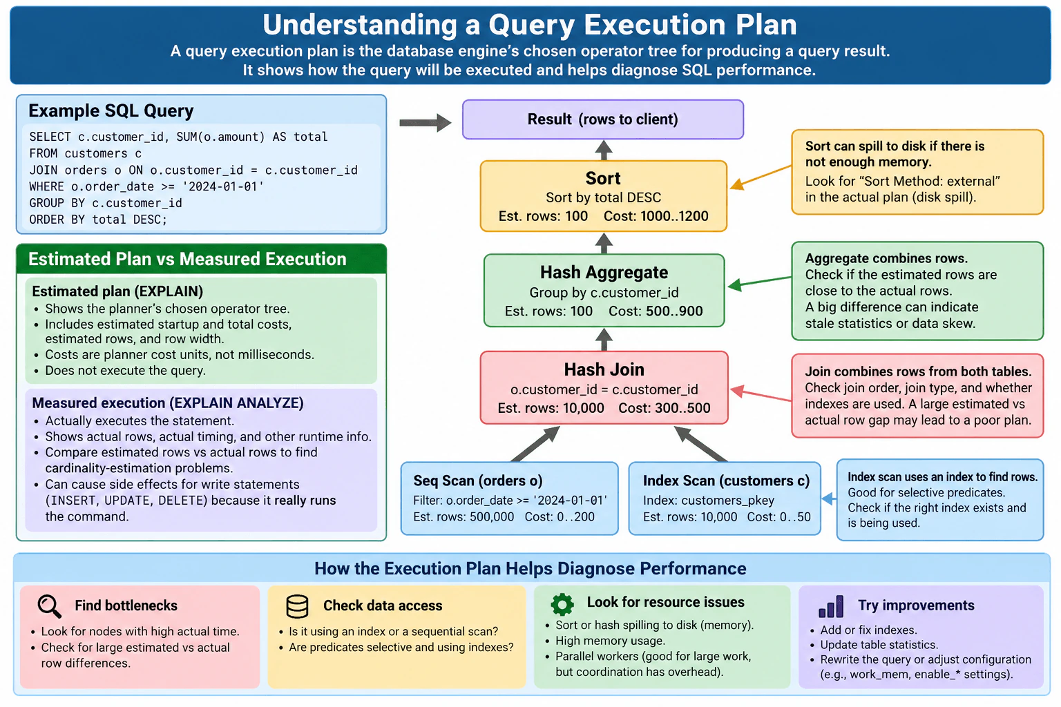
Start with the operator tree. In the diagram's example, the SQL reads orders and customers, joins them on the customer key, groups by customer, sorts by the calculated total, and returns rows to the client. The physical flow is bottom to top: a sequential scan of orders and an index scan of customers feed a hash join; the hash join feeds a hash aggregate; the aggregate feeds a sort; and the sort produces the final result.
Each box represents an operator. A sequential scan reads rows from a table and applies the date predicate o.order_date >= '2024-01-01'. The customer side uses the customers_pkey index. The hash join combines matching rows from the two inputs. The hash aggregate groups by c.customer_id and computes the aggregate. The final sort orders the grouped rows by total descending.
The plan helps you inspect access paths and predicates. For example, you can see whether a table is read with a sequential scan or an index scan, whether the expected predicate is being applied, and whether the chosen index makes sense for the number of rows being retrieved. An index is not automatically better: when a large part of a table must be read, a sequential scan can be the appropriate choice.
Estimated and measured plans serve different purposes. An estimated EXPLAIN plan shows the planner's chosen operators and estimates such as startup cost, total cost, estimated rows, and row width without executing the query. Planner costs are relative cost units, not milliseconds. Measured execution with EXPLAIN ANALYZE actually runs the statement and adds runtime information such as actual row counts and actual timing. Because it really executes the statement, using it with INSERT, UPDATE, or DELETE can cause real side effects.
A key diagnostic is estimated rows versus actual rows. If an operator is expected to produce a small number of rows but actually produces far more, later choices such as join strategy, aggregation, or sorting may be based on a poor cardinality estimate. A large mismatch can point to stale statistics, skewed data, correlated values, or a predicate whose selectivity was estimated badly.
Next, find the dominant runtime work. Look for operators with high actual time, unexpectedly large row counts, or repeated execution. Check whether a sequential scan is processing many unnecessary rows, whether the join type and join order fit the inputs, whether the intended indexes are used, and whether predicates reduce data early enough.
Memory behavior matters too. Sort and hash operators need working memory. If their data does not fit, they can spill intermediate work to disk, which adds extra I/O and rereading or merge work. The diagram highlights an external sort as a sign of disk spill and also calls out hash spilling. More memory can reduce spill in some cases, but first verify that memory pressure is the real cause instead of changing configuration blindly.
Parallelism can also appear in an execution plan. Multiple workers may speed up suitable large operations, but coordination has overhead. Parallelism helps only when there is enough independent work and the added coordination cost is justified, so more workers are not automatically faster.
A practical tuning loop is: confirm the query result is correct, inspect the plan, locate the dominant operator, compare estimates with actual rows and timing, classify the cause as access path, predicate selectivity, join choice, stale statistics, memory or spill, or parallelism overhead, change one relevant lever, and run the same workload again. Useful changes may include adding or correcting an index, updating table statistics, rewriting the query or predicate, or adjusting an appropriate memory or execution setting. Finally, verify that the output is unchanged and that measured performance actually improved.
Technical Approach
Confirm that the SQL result is correct and define the performance target.
Read the execution plan from the data-producing scans toward the final result.
When safe, collect measured execution so actual rows and timing are available.
Compare estimated rows with actual rows to detect cardinality-estimation problems.
Locate the operator responsible for the largest measured runtime or unexpectedly large row volume.
Classify the likely cause: inefficient access path, predicate selectivity, join choice, stale statistics, memory pressure, spill, or parallelism overhead.
Change one relevant lever, such as an index, statistics, query shape, predicate, or appropriate execution setting.
Re-run the same representative workload and compare the plan and runtime evidence.
Validate that the query returns the same correct result after the change.
Practical Insights
There is no single Big-O complexity for the whole SQL query because each operator performs different work. A sequential scan may read a large part of a table, while a selective index scan can avoid much of that reading. A hash join builds and probes hash structures, a hash aggregate keeps state for groups, and a sort needs CPU and memory. If sorting or hashing exceeds available working memory, temporary data may spill to disk and add extra I/O. Parallel workers can reduce elapsed time when enough independent work exists, but they also add coordination overhead. The practical costs to inspect are rows processed, CPU time, memory, temporary disk I/O, and parallel coordination.
Why Interviewers Ask This
Interviewers want to know whether you can reason about how a database actually executes SQL rather than looking only at the query text. A strong answer shows that you understand operator trees, scans, joins, aggregates, sorts, predicates, indexes, estimated versus actual rows, planner costs, runtime timing, memory pressure, spills, and parallelism, and that you can use this evidence to find the dominant performance problem before tuning.
Common interview mistakes
Common mistakes include treating planner cost as elapsed milliseconds, assuming the operator with the highest estimated cost must be the measured runtime bottleneck, looking only at SQL text instead of the operator tree, assuming an index scan is always faster than a sequential scan, ignoring large estimated-versus-actual row mismatches, overlooking predicates and row counts flowing between operators, adding indexes without measuring the result, assuming every spill should be solved only by adding memory, and assuming more parallel workers always make a query faster. Another serious mistake is running EXPLAIN ANALYZE on a write statement without realizing that the statement is actually executed.
Interview tip
Explain the plan from the scans toward the final result and connect every operator to evidence. Mention estimated versus actual rows, actual timing, indexes and predicates, memory and spills, and parallelism. Finish with a disciplined loop: locate the dominant operator, make one targeted change, rerun the same workload, and verify both performance and correctness.
Interviewer may ask next
What is the difference between an estimated execution plan and EXPLAIN ANALYZE?
An estimated plan shows the optimizer's chosen operators and estimates such as row counts and planner costs without executing the query. EXPLAIN ANALYZE actually runs the statement and adds measured information such as actual rows and actual timing. This makes it useful for finding cardinality-estimation errors and runtime bottlenecks, but it must be used carefully because write statements are really executed and can have side effects.
What would you investigate if estimated rows are very different from actual rows?
I would identify the first operator where the mismatch becomes large and inspect the predicates and data distribution feeding it. The cause may be stale statistics, skewed values, correlated columns, or selectivity assumptions that do not match the real data. That bad estimate can lead the optimizer to choose an inefficient join or access strategy. I would address the statistics or query issue, rerun the same workload, and verify that estimates are closer to actual rows while the result remains unchanged.
44. When does bitmap indexing improve SQL retrieval?PerformanceEasy
i Question Details
Use frequently queried, low-cardinality columns in an infrequently updated table to explain bitmap operations and workload suitability.
Short Interview Answer (30-60 seconds)
Bitmap indexes are most useful for frequently filtered, low-cardinality columns in read-heavy or infrequently updated tables. Each value has a bitmap of matching rows, and conditions can be combined with bitwise AND, OR, or NOT before fetching the qualifying rows.
Detailed Explanation
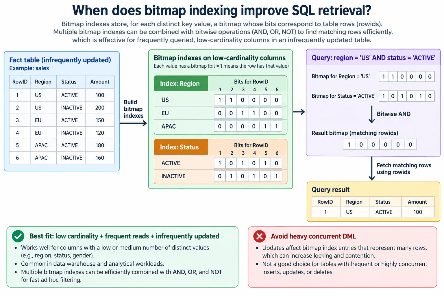
Bitmap indexing is useful when queries repeatedly filter on columns with only a small number of distinct values and the indexed table changes infrequently. Instead of identifying matching rows through many separate conventional index entries, a bitmap index represents row membership with bits. For a query such as region = 'US' AND status = 'ACTIVE', the relevant bitmaps can be combined with a bitwise AND. The resulting bitmap identifies the matching rowids, and the database then fetches only those qualifying rows. This is especially suitable for read-heavy analytical and data-warehouse-style workloads.
Useful Questions to Ask the Interviewer
Is the table mainly read-heavy, or does it receive frequent concurrent inserts, updates, and deletes?
Are the candidate columns used frequently in WHERE filters and do they have relatively few distinct values?
Do queries commonly combine several low-cardinality predicates with AND, OR, or similar Boolean conditions?
How to Explain It in an Interview
Start with the workload conditions: bitmap indexes are a strong fit when the indexed columns have low cardinality, those columns are queried frequently, and the table is read-only, slowly changing, or otherwise infrequently updated.
In the diagram, the sales table has two low-cardinality columns: Region and Status. Region contains US, EU, and APAC, while Status contains ACTIVE and INACTIVE. The bitmap index stores one bitmap for each distinct value. A 1 means that the row has that value, while a 0 means that it does not.
For Region = 'US', the bitmap is 1 1 0 0 0 0. For Status = 'ACTIVE', the bitmap is 1 0 1 0 1 0. Applying a bitwise AND produces 1 0 0 0 0 0. The only set bit corresponds to RowID 1, so the query result is the row with Region US, Status ACTIVE, and Amount 100.
The important performance benefit is that multiple low-cardinality predicates can be combined at the bitmap level before table rows are fetched. AND keeps rows that satisfy every condition, OR can combine alternative conditions, and NOT can exclude a matching set where the database supports that bitmap operation.
The main trade-off is write behavior. Bitmap index entries represent sets of rows for each indexed value, so changing indexed values requires bitmap maintenance and can create locking or contention. That makes bitmap indexes a poor choice for tables with frequent or highly concurrent inserts, updates, or deletes.
The practical rule is therefore: use bitmap indexes for frequently queried, low-cardinality columns in read-heavy or infrequently updated analytical tables, especially when queries combine several such predicates. Low cardinality by itself is not enough.
Technical Approach
Identify columns that appear frequently in query filters.
Check whether those columns have low cardinality relative to the table.
Confirm that the table is read-heavy, read-only, or infrequently updated rather than subject to heavy concurrent DML.
Build or use a bitmap for each relevant distinct indexed value.
For a multi-condition query, select the bitmap for each predicate.
Combine the bitmaps with the required Boolean operation, such as AND when all conditions must match.
Use the set bits in the result bitmap to identify matching rowids and fetch those rows.
Validate that the read-performance benefit is worth the additional index-maintenance and concurrency cost.
Practical Insights
Bitmap indexes trade some storage and write-maintenance cost for efficient filtering. A bitmap can represent many row-membership decisions compactly, and bitwise operations can combine predicates without examining every table row first. That can reduce the number of rows fetched for read-heavy analytical queries. The main downside is maintenance: inserts, updates, and deletes affecting indexed values must update the bitmap structures and can cause contention in highly concurrent workloads. This optimization is primarily about index access and row filtering; the diagram does not involve a distributed shuffle, network exchange, spill, or streaming state.
Why Interviewers Ask This
Interviewers want to see whether you understand the workload characteristics that make bitmap indexes useful, how bitmaps represent row membership, how multiple predicates can be combined efficiently, and why frequent or highly concurrent DML makes bitmap indexing a poor fit.
Common interview mistakes
A common mistake is assuming that every low-cardinality column should have a bitmap index. Workload matters too: the column should be queried frequently and the table should not receive heavy concurrent DML. Another mistake is saying the bitmap stores the row data itself; it represents which rows match each indexed value. Candidates may also forget the key advantage of combining several bitmap predicates before fetching rows. Finally, do not promise that a bitmap index will always beat a full scan or another index type, because the best access path still depends on the database, data distribution, selectivity, and query.
Interview tip
Lead with the three conditions: low cardinality, frequent filtering, and infrequent updates. Then walk through one small AND example using the Region and Status bitmaps, show how the result identifies RowID 1, and finish with the heavy-DML contention trade-off.
Interviewer may ask next
Why are bitmap indexes useful when a query filters on several low-cardinality columns?
Each indexed value has a bitmap identifying which rows contain that value. The database can combine the relevant bitmaps with Boolean operations before fetching table rows. In the diagram, Region = 'US' gives 1 1 0 0 0 0 and Status = 'ACTIVE' gives 1 0 1 0 1 0. Their bitwise AND is 1 0 0 0 0 0, leaving only RowID 1 as the match.
Why are bitmap indexes usually a poor fit for tables with heavy concurrent DML?
Bitmap index entries represent sets of rows for each indexed value, so changing indexed values requires maintaining those bitmap structures. In database implementations that use locking around bitmap index entries, concurrent updates can affect many represented rows and increase contention. For that reason, bitmap indexing is generally better suited to read-heavy or infrequently modified analytical tables than to highly concurrent transactional workloads.
45. How do Snowflake’s result, metadata, and warehouse caches affect SQL execution?PerformanceMedium
i Question Details
Distinguish reused query results from metadata-only work and cached data blocks.
Short Interview Answer (30-60 seconds)
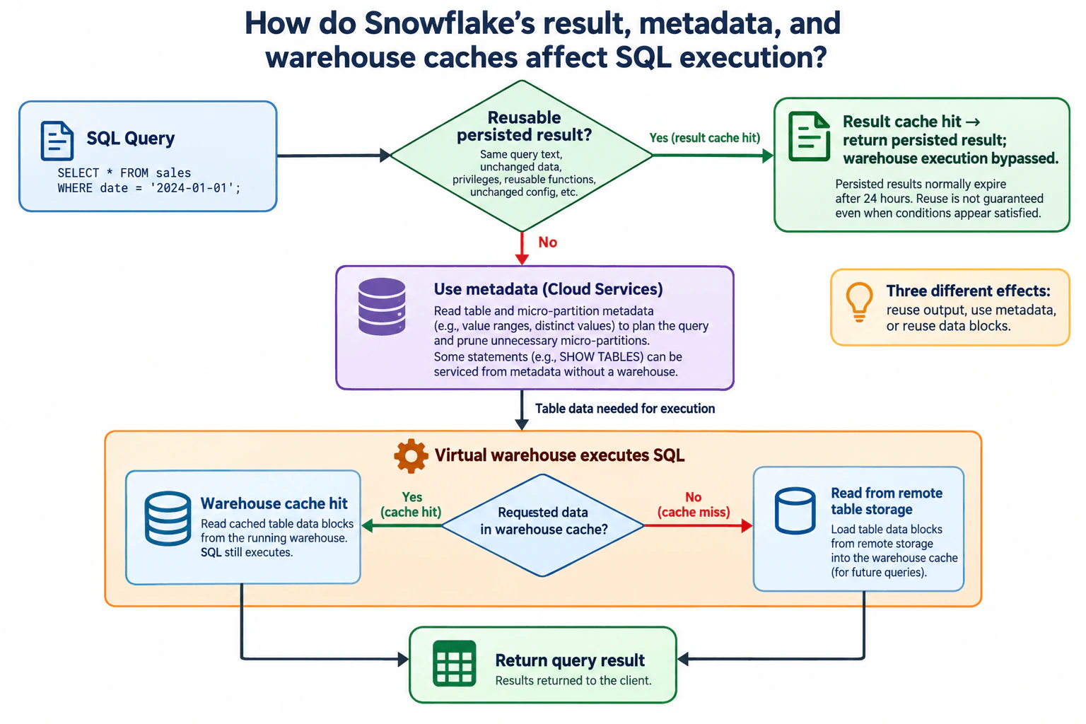
A reusable persisted result can bypass warehouse execution. Otherwise, Snowflake uses Cloud Services metadata for planning and pruning, and some metadata-only work needs no warehouse. If SQL must execute, the warehouse can reuse cached table data; cache misses require reads from remote storage.
Detailed Explanation
Snowflake uses three distinct forms of reuse, and each affects a different point in SQL execution. A reusable persisted result can satisfy the request before warehouse execution starts. If no result is reused, Cloud Services uses table and micro-partition metadata to plan the query and prune unnecessary micro-partitions; some metadata-only statements can be handled without a warehouse. When table data is required, a virtual warehouse executes the SQL. It can read needed table data from its warehouse cache, or fetch missing data from remote storage and cache it for later queries.
Useful Questions to Ask the Interviewer
Are you asking me to distinguish persisted result reuse, metadata processing in Cloud Services, and the virtual warehouse data cache?
Should I focus on which paths bypass warehouse execution versus which only reduce work during planning or execution?
Should I also explain the main conditions that can prevent persisted-result reuse?
How to Explain It in an Interview
Start with the strongest distinction: a persisted query result is not the same thing as warehouse-cached table data.
For a query such as SELECT * FROM sales WHERE date = '2024-01-01';, Snowflake can first determine whether an eligible persisted result from a previous execution can be reused. Reuse depends on conditions such as the query matching the previous query, the referenced data remaining unchanged, required privileges still being valid, and the query being eligible for reuse. If Snowflake can reuse the result, it returns the already computed result and bypasses virtual warehouse execution. Persisted results are retained for a limited period, normally 24 hours, and reuse is not guaranteed simply because a similar query ran recently.
If there is no reusable persisted result, Cloud Services uses metadata about tables and micro-partitions to plan the query. That metadata includes information such as value ranges and distinct-value information that can help Snowflake eliminate micro-partitions that cannot contain qualifying rows. This is metadata work; it is different from reading the table's actual data. Some statements that only need metadata, such as SHOW TABLES, can be serviced without virtual warehouse execution.
If the query needs table data, the virtual warehouse executes the SQL. During execution, Snowflake can reuse table data already present in that running warehouse's cache. On a warehouse-cache hit, the warehouse reads cached table data and the SQL still executes; the benefit is avoiding some remote table-storage I/O. On a warehouse-cache miss, the warehouse reads the required table data from remote storage and that data can populate the warehouse cache for later queries.
The final distinction is therefore simple: persisted-result reuse reuses the completed output and can skip warehouse execution; metadata reuse supports planning, pruning, and metadata-only work; warehouse caching reuses table data while SQL is still executing. A fast repeated query should not automatically be interpreted as proof of a better execution plan because different cache paths can perform very different amounts of work.
Technical Approach
Determine whether an eligible persisted result can be reused.
If it can, return the persisted result and bypass virtual warehouse execution.
If it cannot, use Cloud Services metadata to plan the query and prune unnecessary micro-partitions.
If the statement requires only metadata, return the metadata-based result without warehouse execution.
If table data is required, execute the SQL on a virtual warehouse.
Read required table data from the warehouse cache when present.
On a warehouse-cache miss, read the required data from remote table storage and allow it to populate the warehouse cache for later queries.
Return the final query result to the client.
Practical Insights
The three mechanisms reduce different kinds of work. A persisted-result hit avoids the query's warehouse execution altogether, so it can save the most compute for that request. Metadata processing happens in Cloud Services and can reduce the amount of table data that later needs to be scanned by pruning irrelevant micro-partitions; metadata-only statements may need no warehouse. When SQL executes, a warehouse-cache hit reduces remote storage reads but does not remove CPU, memory, join, aggregation, or other execution work. A cache miss requires remote data reads before the warehouse can process the needed data. Performance tests should therefore control for cache state before comparing runtimes.
Why Interviewers Ask This
This question tests whether a candidate can distinguish three different Snowflake performance mechanisms: reusing a completed query result, using Cloud Services metadata for planning and metadata-only work, and reusing cached table data during virtual warehouse execution. The important judgment is knowing which mechanism can bypass warehouse execution entirely and which mechanisms only reduce planning work or remote storage I/O.
Common interview mistakes
A common mistake is calling all three mechanisms the result cache. A persisted-result hit can bypass warehouse execution, while a warehouse-cache hit only avoids some remote storage reads and the SQL still executes. Another mistake is treating metadata as cached table data: Cloud Services metadata describes tables and micro-partitions and supports planning and pruning, but it is not the table data reused by a warehouse. Candidates also often assume that any repeated query will reuse a persisted result, or that a faster second execution proves the optimizer created a better plan. Cache state must be separated from plan quality.
Interview tip
Explain the three boundaries in order: result cache means reuse the completed result and potentially skip warehouse execution; metadata means plan, prune, or answer metadata-only work; warehouse cache means reuse table data during execution. Emphasize that only the first mechanism reuses the complete query output.
Interviewer may ask next
What is the difference between a Snowflake persisted-result hit and a warehouse-cache hit?
A persisted-result hit returns an already computed query result and can bypass virtual warehouse execution. A warehouse-cache hit occurs when the query still executes on a warehouse; the warehouse reuses cached table data instead of reading that data from remote storage. The first avoids query execution, while the second mainly reduces storage I/O during execution.
Why can two executions of the same SQL have different runtimes even when the SQL text has not changed?
They can take different cache paths. One execution might reuse a persisted result and avoid warehouse execution. Another might execute but find the required table data in the warehouse cache. A colder execution may need remote storage reads. Metadata pruning can also reduce the amount of table data that needs to be scanned. Because these mechanisms change the physical work performed, runtime differences alone do not prove that the SQL execution plan improved.
46. How does SQL Server lock escalation affect concurrent DML?PerformanceMedium
i Question Details
Explain escalation triggers, blocking impact, and controls whose effectiveness can be measured.
Short Interview Answer (30-60 seconds)
SQL Server can escalate many fine-grained key or page locks to a coarser table lock when the lock-count threshold or lock-memory pressure is reached. That reduces lock-management overhead but can block incompatible concurrent DML. Reduce lock footprint, batch large changes, and verify the effect with escalation events and blocking waits.
Detailed Explanation
SQL Server normally uses fine-grained locks so concurrent sessions can work on different rows with good concurrency. A large DML statement can accumulate many key or page locks. When a statement reaches the lock-count escalation threshold on one table reference, or the instance reaches a lock-memory threshold, SQL Server can replace those locks with a coarser table lock. That reduces lock-management overhead but increases the scope of contention. An incompatible INSERT, UPDATE, or DELETE can then wait while the escalated lock is held, so the main performance impact is reduced concurrent DML throughput.
Useful Questions to Ask the Interviewer
Is the observed problem frequent lock escalation, long blocking duration, or both?
Are large modifications executed as one long transaction or already divided into smaller transactions?
Is the affected table partitioned, making LOCK_ESCALATION = AUTO relevant?
Can we capture Extended Events and request-level wait information before and after the change?
How to Explain It in an Interview
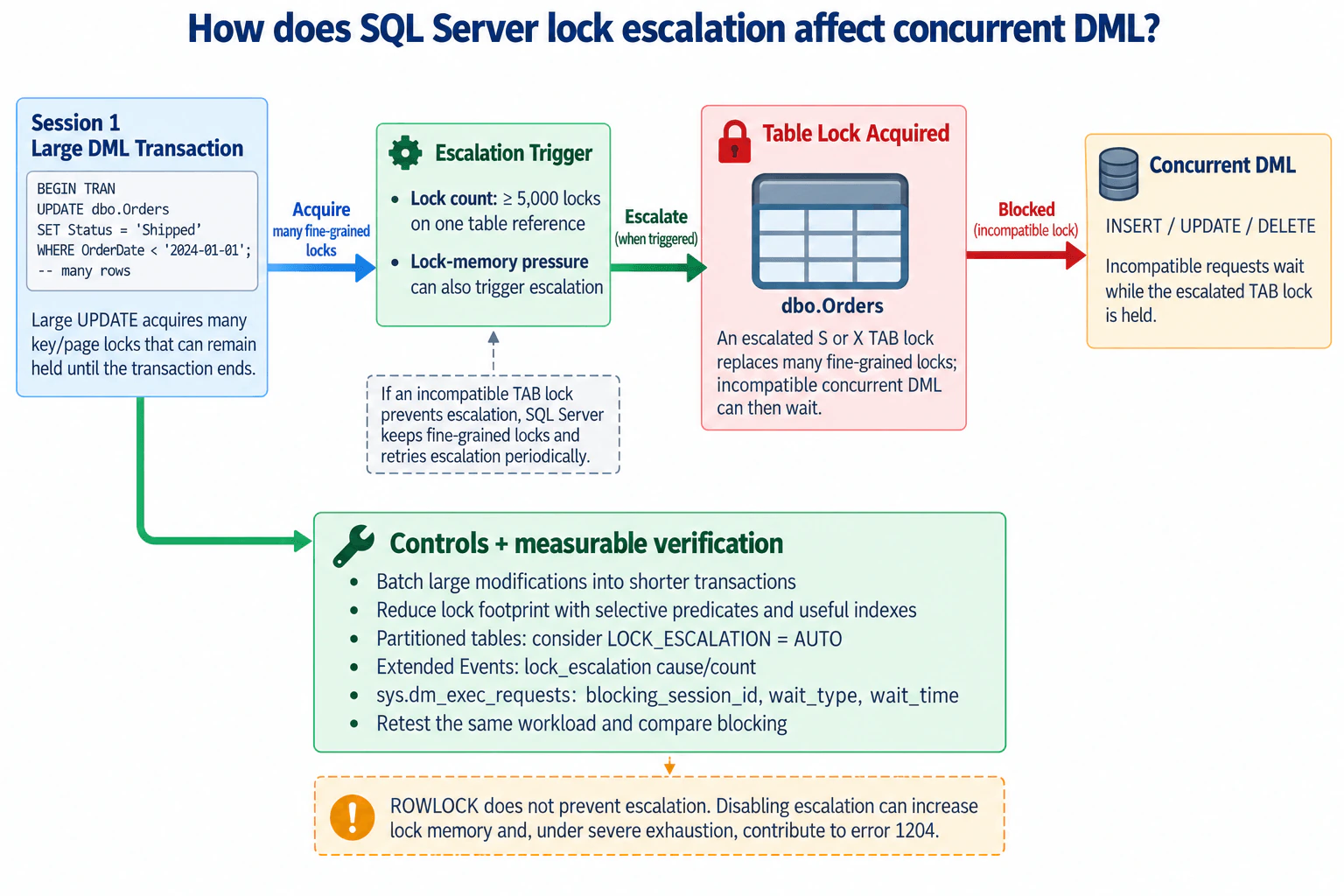
Use the dbo.Orders flow from the diagram. Session 1 performs a large UPDATE and acquires many fine-grained key or page locks. In the traditional locking path shown, those locks can accumulate during the transaction. SQL Server triggers lock escalation when a single Transact-SQL statement acquires at least 5,000 locks on a single table reference, or when instance lock-memory thresholds are exceeded. learn.microsoft.com
If escalation succeeds, SQL Server converts the applicable intent lock to a full table lock and releases lower-granularity locks protected by it. The resulting S or X TAB lock is strong enough for the locks being replaced. For the UPDATE workload in the diagram, an X table lock is the important blocking case. Incompatible concurrent INSERT, UPDATE, or DELETE requests can then wait even if they intended to modify different rows. The benefit is lower lock-manager overhead; the trade-off is a much larger blocking scope and lower concurrency. learn.microsoft.com
Escalation does not necessarily succeed immediately. If another transaction holds an incompatible TAB lock, SQL Server keeps acquiring fine-grained locks and retries escalation periodically rather than waiting solely for the escalation attempt. Current documentation states that after a lock-conflict failure, another escalation attempt is triggered for each additional 1,250 locks acquired. learn.microsoft.com
The first control is to reduce the number of locks a transaction needs. Split large modifications into shorter transactions when business semantics allow it. Use selective predicates and useful indexes so SQL Server scans or looks up fewer rows and therefore acquires fewer locks. For partitioned tables, LOCK_ESCALATION = AUTO allows escalation to the HoBT level associated with a partition instead of necessarily escalating to a whole-table lock. learn.microsoft.com
Measure whether the change actually helps. Capture the sqlserver.lock_escalation Extended Event to observe escalation activity. The event can expose details such as escalation cause and escalated lock count. Use sys.dm_exec_requests to inspect blocking_session_id, wait_type, and wait_time for actively executing requests. Then rerun the same representative workload under comparable concurrency and compare escalation frequency, blocking duration, waits, and throughput. learn.microsoft.com
Do not assume ROWLOCK prevents escalation; it only affects initial lock acquisition. Also, disabling or continually preventing escalation can allow large numbers of fine-grained locks to consume substantial lock memory. If SQL Server can no longer allocate lock resources, error 1204 can occur. learn.microsoft.com
One modern SQL Server nuance is optimized locking. When optimized locking is enabled, row and page locks are generally released much earlier for modifications and lock escalation is far less likely. Therefore, first determine whether optimized locking applies before assuming the traditional long-lived row/page-lock behavior shown in the diagram. This does not change the diagram's escalation mechanism; it changes how often that mechanism is likely to be reached. learn.microsoft.com
Technical Approach
Reproduce the representative concurrent DML workload and confirm the blocking symptom.
Capture sqlserver.lock_escalation events and inspect sys.dm_exec_requests for blocking_session_id, wait_type, and wait_time.
Determine whether escalation is driven by the per-table-reference lock-count threshold or lock-memory pressure.
Reduce the lock footprint with shorter transactions, selective predicates, and useful indexes.
If the table is partitioned, evaluate LOCK_ESCALATION = AUTO when HoBT-level partition escalation is appropriate.
Retest the same workload under comparable concurrency.
Compare escalation activity, blocked duration, waits, and throughput.
Confirm transaction semantics and result correctness remain unchanged, while checking that lock-memory use remains safe.
Practical Insights
Fine-grained locking uses more lock-manager memory because SQL Server must track many individual key or page locks, but it usually allows greater concurrency. Escalating to one table lock reduces that bookkeeping overhead, but incompatible sessions can wait longer because the lock covers a larger scope. Smaller transactions and better predicates or indexes can reduce the number of locks and blocking duration, but batching adds transaction and operational overhead. Preventing escalation too aggressively can increase lock-memory consumption and, in extreme cases, lead to failure to allocate additional lock resources.
Why Interviewers Ask This
Interviewers want to see whether you understand why SQL Server trades many fine-grained locks for a coarser lock, how that trade-off can reduce concurrent DML, what triggers escalation, how a failed escalation attempt behaves, and how to reduce and measure harmful escalation without blindly applying lock hints or disabling the mechanism.
Common interview mistakes
Common mistakes are treating 5,000 as a server-wide lock count instead of a per-statement threshold on a single table reference; ignoring lock-memory-triggered escalation; assuming escalation always succeeds immediately; thinking ROWLOCK prevents escalation; forgetting that an escalated table lock can block sessions targeting different rows; disabling escalation without considering lock-memory growth and error 1204; batching without checking transaction semantics; changing indexes or escalation settings without measuring the original blocking; and claiming success without retesting the same representative workload and concurrency. On modern deployments, another mistake is ignoring whether optimized locking is enabled.
Interview tip
Present the answer as a trade-off: many fine-grained locks preserve concurrency but cost lock memory; escalation reduces lock overhead but increases blocking scope. Then walk through trigger, table-lock impact, failed-escalation behavior, targeted controls, measurable verification, and the memory-risk trade-off. Mention optimized locking only as a modern qualification after explaining the core mechanism.
Interviewer may ask next
What happens if SQL Server tries to escalate but another session holds an incompatible table lock?
The escalation attempt fails at that time. SQL Server continues acquiring fine-grained row, key, or page locks as needed and periodically retries escalation. Current SQL Server documentation states that after a conflict prevents escalation, another attempt is triggered for each additional 1,250 locks acquired. This avoids waiting solely for the escalation request, although the transaction can continue consuming lock memory.
Why not simply disable lock escalation for a heavily updated table?
Disabling escalation can reduce some table-lock blocking, but it can leave SQL Server tracking very large numbers of fine-grained locks. That increases lock-memory consumption, and if additional lock resources cannot be allocated, error 1204 can occur. A safer approach is usually to reduce lock footprint, use shorter transactions when semantics permit, measure blocking, and use LOCK_ESCALATION = AUTO for appropriate partitioned-table workloads.
47. How would you diagnose tempdb allocation contention?PerformanceHard
i Question Details
Distinguish PFS/GAM latch contention from storage latency and evaluate SQL Server file configuration.
Short Interview Answer (30-60 seconds)
I would classify the waits first. PAGELATCH_* on tempdb PFS, GAM, or SGAM pages means in-memory allocation contention; PAGEIOLATCH_* points to storage latency. For latch contention, I would check file count and equal sizing, adjust tempdb data files if needed, and then rerun the same workload.
Detailed Explanation
tempdb allocation contention happens when many SQL Server sessions compete for shared allocation-map pages while allocating or deallocating temporary pages. The key diagnostic step is separating in-memory latch pressure from slow storage. PAGELATCH_* waits associated with tempdb PFS, GAM, or SGAM pages indicate contention on allocation metadata, whereas PAGEIOLATCH_* waits indicate that sessions are waiting for physical I/O to complete. After proving allocation contention, evaluate the number and size of tempdb data files, make the smallest relevant configuration change, and retest the same representative workload.
Useful Questions to Ask the Interviewer
Which SQL Server version is running?
Are PAGELATCH_* or PAGEIOLATCH_* waits dominant during the slowdown?
Do the waiting resources belong to tempdb, whose database_id is 2?
How many tempdb data files exist, and are they equally sized?
Does the slowdown correlate with high concurrent tempdb allocation activity, elevated storage latency, or both?
How to Explain It in an Interview
I would diagnose this as an evidence-first problem rather than immediately adding tempdb files.
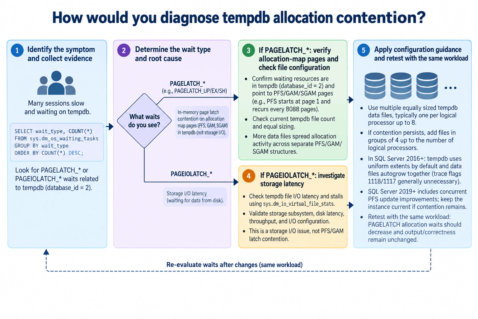
First, I would inspect current waiting tasks and aggregate wait types. The important split is between PAGELATCH_* and PAGEIOLATCH_* waits associated with tempdb.
If PAGELATCH_* waits dominate, I would inspect the waiting resources and verify that they belong to tempdb and point to allocation-map pages such as PFS, GAM, or SGAM. These are shared allocation structures. A PFS page starts at page 1 in each database file and recurs every 8088 pages, so the diagnostic should not assume that only the first allocation page can become hot. PAGELATCH_* contention here is an in-memory page-latch problem, not evidence of slow storage.
I would then inspect the current tempdb data-file configuration. Multiple equally sized data files spread allocation activity across separate allocation-map structures. A common starting point is one tempdb data file per logical processor up to eight files. If contention remains, additional files can be added in groups of four up to the number of logical processors instead of adding an arbitrary number at once.
If PAGEIOLATCH_* waits dominate instead, I would follow the storage branch. I would inspect tempdb file I/O latency and stalls with sys.dm_io_virtual_file_stats and investigate disk latency, throughput, and I/O configuration. PAGEIOLATCH_* means SQL Server is waiting on physical I/O, so adding tempdb files solely to address allocation-map latch contention would target the wrong mechanism.
Version behavior matters as well. Starting with SQL Server 2016, tempdb uses uniform extents by default and its data files autogrow together, so the older trace-flag 1118 and 1117 guidance is generally unnecessary for tempdb. SQL Server 2019 and later also include concurrent PFS update improvements, although the instance should still be measured if contention remains.
Finally, I would change one relevant lever and rerun the same representative workload. I would compare the same wait evidence and confirm that PAGELATCH allocation waits decrease. I would also verify that the workload still produces the same correct result. The trade-off is operational: additional files increase file-management complexity, so the goal is enough equally sized files to reduce measured allocation contention rather than the largest possible file count.
Technical Approach
Observe or reproduce the slowdown with a representative workload.
Inspect current waiting tasks and aggregate wait types.
Determine whether PAGELATCH_* or PAGEIOLATCH_* is dominant for tempdb.
For PAGELATCH_, verify that waiting resources belong to tempdb and correspond to PFS, GAM, or SGAM allocation-map pages.
Inspect the current tempdb data-file count and whether the files are equally sized.
If allocation contention is confirmed, use multiple equally sized tempdb data files, typically starting with one per logical processor up to eight.
If contention remains, add files in groups of four up to the number of logical processors rather than changing unrelated settings.
For PAGEIOLATCH_, inspect tempdb file I/O stalls and storage latency instead of treating the problem as allocation-latch contention.
Account for SQL Server version-specific tempdb behavior before applying older trace-flag guidance.
Rerun the same workload, compare the same wait evidence, and verify that correctness remains unchanged.
Practical Insights
This is not an algorithm with Big-O complexity. The important costs are latency, storage activity, and operational complexity. Too few tempdb files can leave many sessions contending on the same allocation-map structures. Adding equally sized files can spread that activity, but adding files blindly creates more configuration and monitoring work and does not solve slow storage. PAGEIOLATCH_* problems consume I/O time and must be investigated through file stalls, latency, throughput, and the storage path. The safest approach is to change one relevant lever and compare the same representative workload before and after.
Why Interviewers Ask This
This tests whether the candidate can distinguish SQL Server in-memory allocation latch contention from storage latency instead of treating every tempdb slowdown as a disk problem. It also tests whether they can connect wait evidence to PFS, GAM, and SGAM allocation structures, evaluate tempdb file configuration, apply a targeted mitigation, understand version-specific improvements, and validate the change with the same workload.
Common interview mistakes
Common mistakes include assuming every tempdb performance problem is a disk problem; treating PAGELATCH_* and PAGEIOLATCH_* as equivalent; looking only at aggregate waits without verifying that the waiting resources belong to tempdb; assuming only the first PFS page can become a hotspot; adding many tempdb files before proving allocation contention; using unequal data-file sizes; applying old trace-flag advice without considering the SQL Server version; and declaring success without rerunning the same workload and comparing the same wait evidence.
Interview tip
Present the answer as evidence, classification, physical cause, targeted change, and retest. Explicitly state that PAGELATCH_* is an in-memory latch problem while PAGEIOLATCH_* represents physical I/O waiting; that distinction is the core of the question.
Interviewer may ask next
Why do multiple equally sized tempdb data files reduce allocation contention?
Each tempdb data file has its own allocation-map structures, including PFS, GAM, and SGAM pages. Multiple equally sized files let SQL Server spread allocation activity across those structures instead of concentrating concurrent allocations on a smaller set of hot pages. Equal sizing helps keep allocation opportunities balanced. The goal is to reduce measured latch contention, not simply maximize the number of files.
What would you do if PAGEIOLATCH_* waits are high instead of PAGELATCH_* waits?
I would follow the storage-latency branch rather than treating file count as the primary fix. I would inspect tempdb file I/O stalls with sys.dm_io_virtual_file_stats and evaluate storage latency, throughput, and I/O configuration. PAGEIOLATCH_* indicates waiting for physical I/O, which is a different mechanism from in-memory PFS, GAM, or SGAM latch contention. After any storage change, I would rerun the same workload and compare the same evidence.
48. When would SQL Server Parameter Sensitive Plan optimization be preferable to OPTION (RECOMPILE)?PerformanceHard
i Question Details
Compare parameter-dependent plans, feature eligibility, execution frequency, and compilation CPU.
Short Interview Answer (30-60 seconds)
Prefer PSP for eligible, frequently executed parameter-sensitive queries where different parameter ranges benefit from different plans. PSP reuses a cached dispatcher and query variants, avoiding repeated compilation CPU. Use OPTION (RECOMPILE) when PSP is unavailable or per-execution compilation is acceptable.
Detailed Explanation
The decision is about balancing parameter-specific plan quality against compilation cost. A parameterized query over nonuniform data can need different execution plans for different parameter values. PSP handles eligible cases by caching a dispatcher plan and multiple query variants, then routing each execution to an appropriate variant. This is especially useful for frequently executed statements because the compiled variants can be reused. OPTION (RECOMPILE) instead creates a fresh temporary plan for the current values on every execution, which can provide precise optimization but repeatedly consumes compilation CPU.
Useful Questions to Ask the Interviewer
Is the query running on SQL Server 2022 or later with database compatibility level 160 or higher?
Is the statement actually parameter-sensitive, with different parameter values producing materially different cardinalities and optimal plans?
Does the statement meet PSP eligibility requirements, including the predicate form represented in the diagram and the required parameter-sensitive optimization settings?
How frequently does the query execute, and is compilation CPU significant at that frequency?
If PSP is unavailable or ineligible, is the query infrequent enough that per-execution recompilation is an acceptable trade-off?
How to Explain It in an Interview
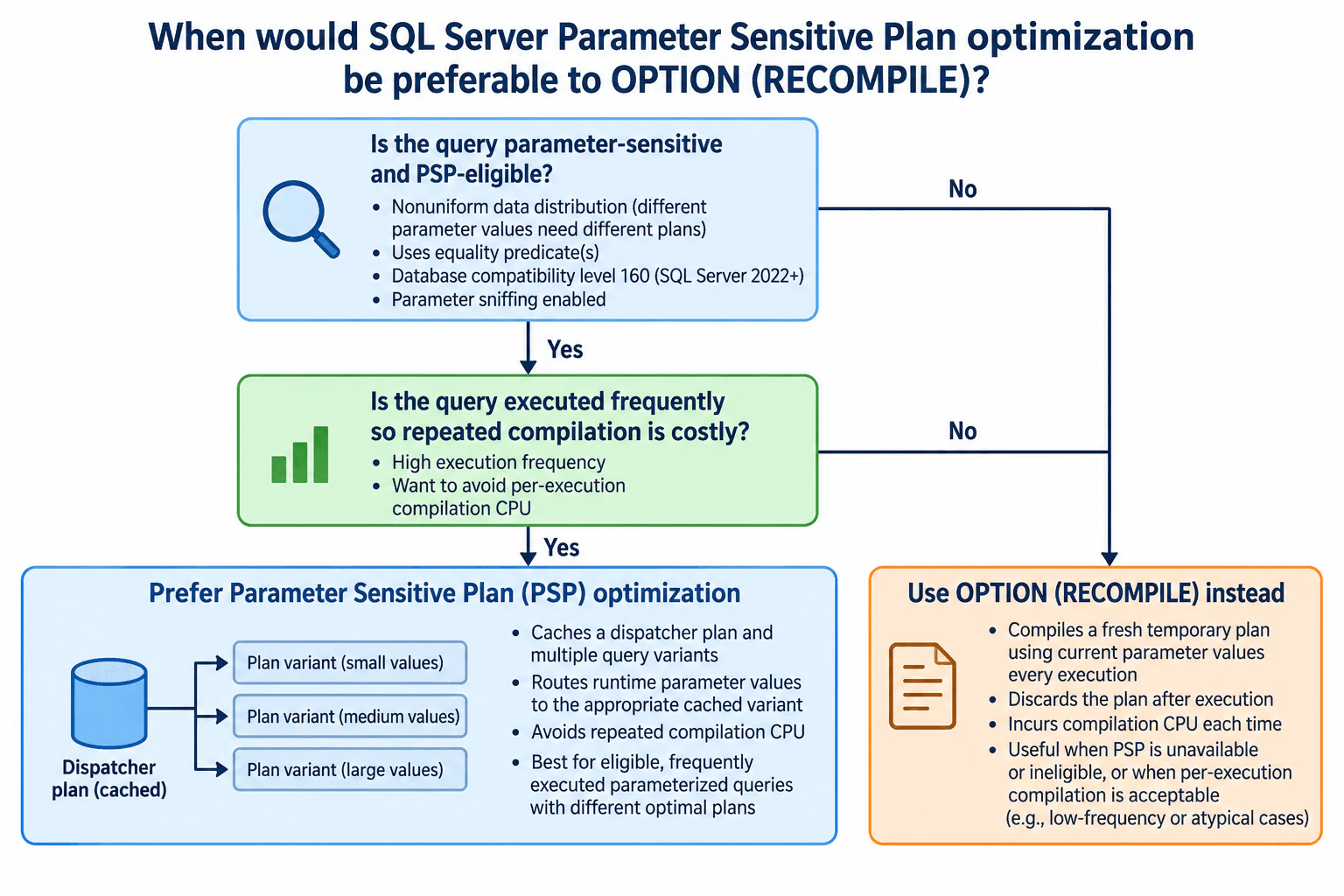
Start with the physical problem: one cached execution plan may not be good for every parameter value when the underlying data distribution is nonuniform. A value that returns few rows can favor a different physical strategy from a value that returns many rows.
For an eligible query, PSP creates and caches a dispatcher plan. The dispatcher evaluates the runtime parameter value and routes the execution to an appropriate cached query variant. The diagram illustrates variants for small, medium, and large cardinality ranges. Treat those labels as a conceptual illustration of parameter-dependent variants, not as a rule that every PSP query must always have exactly three plans.
This makes PSP attractive for frequently executed queries. The dispatcher and variants can be reused across executions, so SQL Server can retain parameter-dependent plan choices without paying the full compilation cost on every call.
OPTION (RECOMPILE) takes the other approach. SQL Server compiles a fresh temporary plan for the current parameter values each time the statement executes, and that plan is discarded afterward. This can produce a plan specialized for the current execution, but repeated executions repeatedly pay compilation CPU.
Therefore, prefer PSP when the query is genuinely parameter-sensitive, meets PSP eligibility requirements, and runs often enough that avoiding repeated compilation matters. Prefer OPTION (RECOMPILE) when PSP is unavailable or ineligible, or when the statement runs infrequently or atypically enough that per-execution compilation CPU is an acceptable cost.
Technical Approach
Confirm parameter sensitivity by checking whether different parameter values produce materially different cardinalities and benefit from different plans.
Check PSP eligibility, including the supported SQL Server version, database compatibility level, applicable parameter-sensitive optimization settings, and eligible predicate form.
Consider execution frequency and determine whether compiling on every execution would create meaningful CPU overhead.
Prefer PSP when the statement is eligible and frequently executed so the dispatcher and query variants can be reused.
Use OPTION (RECOMPILE) when PSP is unavailable or ineligible, or when execution frequency is low enough that repeated compilation is acceptable.
Validate the choice with representative parameter values and compare both execution behavior and compilation overhead.
Practical Insights
The main cost difference is compilation CPU versus plan-cache usage. PSP can keep a dispatcher plan plus multiple query variants in cache, so it may use more plan-cache space, but frequent executions can reuse those compiled plans and avoid recompiling every time. OPTION (RECOMPILE) creates a fresh temporary plan on every execution and discards it afterward, so repeated calls repeatedly consume compilation CPU. The important performance measures are therefore query execution quality, compilation CPU, execution frequency, latency, and plan-cache footprint. Network shuffle, partitioning, and distributed-worker costs are not part of this SQL Server optimizer decision.
Why Interviewers Ask This
This question tests whether you understand the difference between solving parameter sensitivity with reusable cached plan variants and solving it by recompiling for every execution. Interviewers want you to consider parameter-dependent plan quality, PSP feature eligibility, execution frequency, plan-cache behavior, and compilation CPU rather than treating either technique as universally better.
Common interview mistakes
Common mistakes include treating PSP as equivalent to OPTION (RECOMPILE), assuming PSP applies to every parameterized query, ignoring database compatibility and feature eligibility, assuming the diagram's small-medium-large illustration means every query always gets exactly three variants, and ignoring execution frequency. Another mistake is focusing only on execution-plan quality while forgetting that OPTION (RECOMPILE) pays compilation CPU on every execution. PSP should be chosen because its cached variants fit an eligible parameter-sensitive workload, not simply because recompilation exists as an alternative.
Interview tip
Organize the answer around three checks: is the query truly parameter-sensitive, is it PSP-eligible, and is it executed frequently enough that repeated compilation CPU matters? Then contrast PSP's cached dispatcher and variants with OPTION (RECOMPILE)'s fresh per-execution plan.
Interviewer may ask next
How does SQL Server PSP select among different plans at runtime?
PSP uses a cached dispatcher plan. The dispatcher evaluates the runtime parameter value against its parameter-cardinality boundaries and routes the execution to an appropriate cached query variant. This allows different parameter ranges to use different plans without recompiling the statement on every execution.
When could OPTION (RECOMPILE) still be preferable to PSP?
OPTION (RECOMPILE) is appropriate when PSP is unavailable or the statement is not eligible, or when the query executes infrequently enough that compilation CPU is acceptable. It is also useful when the desired behavior is to compile specifically for the current parameter values on every execution instead of reusing cached variants.
49. What is data quality, and how do teams decide whether data is fit for use?Reliability And Data QualityEasy
i Question Details
Define data quality in relation to a stated use case. Explain completeness, consistency, conformity, accuracy, freshness, and uniqueness; measurable rules and thresholds; profiling; ownership; monitoring; failed-record handling; and remediation. Clarify that a dataset can satisfy one consumer's requirements while failing another consumer's.
Short Interview Answer (30-60 seconds)
Data quality means data is good enough for a specific use case. Teams define consumer requirements, profile the data, convert those requirements into measurable rules and thresholds, run checks, handle failed records safely, monitor results, and assign owners to remediate problems. The same dataset can be fit for one consumer but not another.
Detailed Explanation
Data quality describes whether data meets the needs of a stated use case, not whether it is universally good. A team first defines what each consumer needs, such as freshness, completeness, consistency, conformity, accuracy, and uniqueness. It profiles the current dataset, converts those expectations into measurable rules and thresholds, and runs quality checks before serving the data. Failed records follow an explicit handling policy, owners investigate and remediate causes, and quality metrics are monitored over time. Because consumer requirements differ, the same dataset can pass for one consumer and fail for another.
Useful Questions to Ask the Interviewer
What consumer or business use case are we deciding fitness for?
What freshness and completeness thresholds does that consumer require?
What does one row represent, and what key defines uniqueness at that grain?
What authoritative source or reconciliation method should be used to support an accuracy claim?
Should failed rows be quarantined, rejected, or flagged while processing continues?
Who owns the dataset, quality rules, alerts, remediation, and consumer communication?
How to Explain It in an Interview
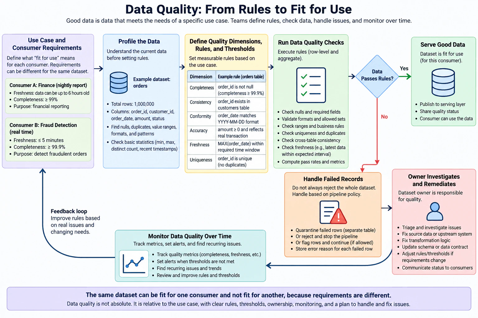
Start with the consumer and the meaning of "fit for use." In the diagram, Consumer A is a nightly finance report that can accept data up to 6 hours old and requires at least 99% completeness. Consumer B is real-time fraud detection, which requires freshness of 5 minutes or less and at least 99.9% completeness. These requirements immediately show why quality is consumer-specific.
Next, profile the current orders dataset before choosing rules. The diagram's example contains 1,000,000 rows with order_id, customer_id, order_date, amount, and status. Profiling looks for nulls, duplicates, value ranges, formats, patterns, minimum and maximum values, distinct counts, and recent timestamps. Profiling describes the current state; it does not by itself decide whether the data is acceptable.
Then convert the consumer requirements into measurable quality dimensions, rules, and thresholds. Completeness asks whether required values are present. The diagram checks that order_id is not null and uses an example completeness threshold of at least 99.9%. Consistency checks whether related data agrees according to the data contract; the diagram shows a cross-table existence check, so the exact field relationship must be the one defined by that contract. Conformity checks whether data follows the expected representation, such as order_date matching YYYY-MM-DD. Accuracy means the value reflects the real-world fact it represents. The diagram shows amount >= 0 and says it should reflect the real transaction. The nonnegative condition is a validity or business-rule check; the real-transaction part requires authoritative reconciliation before calling the value accurate. Freshness checks whether the newest order_date is within the consumer's required time window. Uniqueness checks that order_id has no unwanted duplicates at the declared order grain.
Run the checks at the appropriate level. The diagram includes null and required-field checks, formats and allowed sets, ranges and business rules, uniqueness and duplicate checks, cross-table consistency, freshness, and aggregate pass-rate metrics. The result reaches a decision point: does the data pass the rules for this consumer?
If the answer is yes, publish the dataset to the serving layer, expose its quality status, and allow that consumer to use it. Passing means the dataset satisfied the defined rules and thresholds for that consumer; it does not prove that every possible defect has been excluded.
If the answer is no, follow the approved failure policy instead of silently discarding data. The diagram allows failed rows to be quarantined in a separate table, the pipeline to reject and stop, or rows to be flagged while processing continues when that behavior is explicitly allowed. Store an error reason for each failed row so there is evidence for investigation.
The dataset owner then investigates and remediates the problem. The root cause may be in the source or upstream system, transformation logic, schema, or data contract. After correction, the affected data should be reprocessed or replayed as appropriate and the relevant quality checks should run again before the corrected output is considered fit for use. The owner should also communicate status to affected consumers. Rules or thresholds should change only when business requirements change or an approved policy changes, not merely to make a failed check pass.
Finally, monitor data quality over time. Track metrics such as completeness and freshness, alert when thresholds are missed, identify recurring issues and trends, and review rules when real consumer requirements change. That monitoring feeds back into the use-case requirements and creates the feedback loop shown in the diagram.
The main conclusion is that data quality is not absolute. A dataset can be fit for the nightly finance report but unfit for real-time fraud detection because their freshness and completeness requirements are different. Teams decide fitness by combining a stated use case, measurable rules and thresholds, profiling, safe failure handling, ownership, remediation, and continuous monitoring.
Technical Approach
Identify the consumer and define what "fit for use" means for that use case.
State the record grain and key before defining uniqueness.
Profile the current dataset for nulls, duplicates, ranges, formats, patterns, distinct counts, and recent timestamps.
Translate consumer expectations into measurable rules and thresholds for completeness, consistency, conformity, accuracy, freshness, and uniqueness.
Run row-level and aggregate checks and record observed pass rates or quality metrics.
Compare the observed results with the consumer-specific thresholds.
If the data passes, publish it to the serving layer and expose the quality status.
If it fails, follow the approved policy: quarantine failed rows, reject and stop, or flag and continue when explicitly allowed; record an error reason.
Route the issue to the dataset owner, correct the source, upstream system, transformation, schema, or contract, and reprocess affected data as appropriate.
Monitor quality metrics over time, alert on threshold failures, find recurring issues, and feed lessons back into requirements and rules.
Evaluate fitness separately for each consumer because different consumers can have different thresholds.
Practical Insights
The cost depends on the checks. Null, range, format, and freshness checks can often be evaluated while scanning the data, so CPU and I/O generally grow with the amount of data examined. Exact uniqueness checks may need sorting, hashing, a distinct operation, or a distributed shuffle, which can use more memory, network, and compute. Cross-table consistency checks can require joins and extra reads. Accuracy reconciliation can add reads from an authoritative system and may increase network or database load. Quarantine tables and quality evidence use additional storage. Checks performed before publication also add latency. Sampling can reduce cost but cannot prove that the full dataset is correct. Operational costs include alerts, investigation, remediation, replay, rule maintenance, and communication with consumers.
Why Interviewers Ask This
Interviewers want to see whether you understand that data quality is defined relative to a consumer and use case rather than as an absolute property. A strong answer translates business expectations into measurable checks and thresholds, explains profiling and monitoring, defines safe failure handling, assigns ownership, and describes remediation. It should also distinguish schema or validity checks from true accuracy evidence and explain why the same dataset can be acceptable for one consumer while failing another.
Common interview mistakes
Common mistakes include calling data "high quality" without naming the consumer or use case; applying one threshold to every consumer; defining uniqueness without stating the record grain and key; treating schema or format conformance as proof of accuracy; treating amount >= 0 as sufficient evidence that an amount matches the real transaction; defining freshness without tying it to a consumer-required time window; silently dropping failed records; automatically rejecting the entire dataset when quarantine or approved continuation is the intended policy; changing thresholds simply to make failed checks pass; failing to record error evidence; and assuming shared tooling removes the need for clear data ownership and remediation.
Interview tip
Lead with the idea that data quality is relative to a stated use case. Then walk through consumer requirements, profiling, measurable rules and thresholds, the pass/fail decision, failed-record handling, ownership, remediation, and monitoring. Use the finance-versus-fraud example to show clearly why one dataset can be fit for one consumer and fail another.
Interviewer may ask next
How would you handle a dataset that passes completeness and uniqueness checks but is too stale for one consumer?
Evaluate fitness against that consumer's freshness requirement instead of declaring the dataset generally good. In the diagram, data that is acceptable for the nightly finance report could still fail the real-time fraud consumer, which requires freshness of 5 minutes or less. Mark that consumer-specific quality result as failed, apply the approved publication or quarantine policy, alert the owner, investigate why fresh data is not arriving, remediate the cause, and communicate the status to the affected consumer.
Should every failed data-quality check stop the whole pipeline?
No. Failure behavior should follow the approved policy and the severity of the requirement. The diagram shows three possible responses: quarantine failed rows in a separate table, reject and stop the pipeline, or flag rows and continue when that behavior is explicitly allowed. In every case, record the error reason, route the issue to the owner, correct the root cause, reprocess affected data as appropriate, rerun the relevant checks, and verify the corrected result before treating it as fit for the consumer.
50. Why can SQL Server IDENTITY and SEQUENCE values contain gaps?Reliability And Data QualityEasy
i Question Details
Compare their allocation scope and the effects of rollback, caching, and restart on consecutive numbering.
Short Interview Answer (30-60 seconds)
IDENTITY and SEQUENCE values can have gaps because allocated numbers are not necessarily reused. Rollbacks consume values, caching can lose values after failures, and SEQUENCE values are generated outside transactions. SEQUENCE can also be shared or restarted, so neither feature guarantees consecutive numbering.
Detailed Explanation
SQL Server IDENTITY and SEQUENCE generate numbers for different scopes, but neither guarantees gap-free numbering. IDENTITY is a property of one table column and generates a value during an insert attempt. If that insert is rolled back, the consumed identity value is not reused. SQL Server may also cache identity values, so restart or failure can cause a later insert to receive a higher number. SEQUENCE is an independent schema-bound object, can serve multiple tables, and allocates numbers outside the current transaction, so rollback does not return them.
Useful Questions to Ask the Interviewer
Do you want the comparison to focus only on rollback behavior, or also on caching and restart behavior?
Should I explain the difference between an orderly SQL Server stop and an abnormal shutdown for a cached SEQUENCE?
Do you want me to discuss whether either feature guarantees uniqueness or only consecutive numbering?
How to Explain It in an Interview
Start with allocation scope. IDENTITY belongs to one table column. In the diagram, dbo.Orders.OrderID is defined as INT IDENTITY(1,1). Each insert attempt asks SQL Server for the next identity value for that column. If one transaction inserts a row that receives value 2 and then rolls back, that value is consumed. The next successful insert can receive 3 instead of reusing 2. This is why rollback can create an IDENTITY gap.
Caching is another reason IDENTITY values can jump. SQL Server may cache identity values in memory for performance. If the server restarts or fails, some cached values can be lost. A later INSERT can therefore receive a higher value. The important point is that the generated numbers are not a promise of consecutive numbering.
SEQUENCE has a different allocation scope. It is an independent schema-bound object rather than a property of one table column. The diagram creates dbo.OrderSeq with START WITH 1, INCREMENT BY 1, and CACHE 5. Multiple tables can request numbers from that same object by calling NEXT VALUE FOR dbo.OrderSeq. For example, dbo.Orders can receive 1 and dbo.Invoices can receive 2 from the same sequence.
SEQUENCE values are generated outside the current transaction. Once NEXT VALUE FOR allocates a number, rolling back the surrounding transaction does not put that number back. A value can also be fetched and never inserted into a row, which still leaves a gap.
Caching changes restart behavior for SEQUENCE. CACHE is the default. On an orderly SQL Server stop, the next intended sequence value is saved. After an abnormal shutdown, unused cached sequence values can be lost. In the diagram's example, the sequence cache covers values 200 through 204. After 200 and 201 have been used, SQL Server stops abnormally before 202 through 204 are used. The next value after restart is 205, so 202 through 204 form a gap.
Using NO CACHE reduces gaps caused by loss of cached values, but it does not make the sequence gap-free. Numbers requested and then unused, or numbers consumed by rolled-back transactions, can still be missing. A sequence can also be intentionally changed with ALTER SEQUENCE dbo.OrderSeq RESTART WITH 1000, which changes the next value returned and does not provide consecutive numbering.
The interview conclusion is simple: IDENTITY and SEQUENCE are useful number generators, not gap-free counters. Neither feature guarantees consecutive numbering or uniqueness by itself. If a column must be unique, enforce that requirement with a PRIMARY KEY or UNIQUE constraint. Do not use the absence of gaps as a data-quality invariant.
Technical Approach
Identify the allocation scope: IDENTITY belongs to one table column, while SEQUENCE is an independent schema-bound object that can be shared.
Check when a number is consumed: an IDENTITY value is generated for an insert attempt, while NEXT VALUE FOR allocates a SEQUENCE value independently of row insertion.
Explain rollback: consumed IDENTITY and SEQUENCE values are not returned for reuse.
Explain caching: SQL Server may cache IDENTITY values, and SEQUENCE uses CACHE by default.
Separate restart cases for SEQUENCE: an orderly SQL Server stop saves the next intended value, while an abnormal shutdown can lose unused cached values.
Explain that NO CACHE reduces cache-loss gaps but cannot remove rollback or unused-value gaps.
Mention that a SEQUENCE can be deliberately restarted.
Conclude that generated values should not be treated as a gap-free data-quality rule and uniqueness must be enforced separately.
Practical Insights
Generating an IDENTITY or SEQUENCE value is a small database operation, but the design deliberately trades perfectly consecutive numbering for normal database performance and concurrency. Caching reduces repeated persistent writes and can make sequence generation cheaper, but unused cached sequence values can be lost after an abnormal shutdown. NO CACHE reduces that specific risk by persisting sequence progress more frequently, at the cost of additional disk work. There is usually no meaningful network cost beyond the database request itself. The main operational cost is conceptual: applications, tests, reconciliation jobs, and downstream consumers must not treat missing generated numbers as proof that rows are missing or data is corrupt.
Why Interviewers Ask This
This question checks whether the candidate understands that generated numeric values are allocation mechanisms, not gap-free counters. It also tests the important differences between table-scoped IDENTITY and reusable SEQUENCE objects, transaction rollback behavior, caching, restart behavior, and the need to enforce uniqueness with a PRIMARY KEY or UNIQUE constraint rather than relying on generated numbering.
Common interview mistakes
A common mistake is assuming an IDENTITY value is returned when a transaction rolls back. Another is assuming SEQUENCE values participate in the surrounding transaction; they are generated outside its scope and remain consumed. Candidates also often say every SQL Server restart loses cached SEQUENCE numbers, but the diagram correctly distinguishes an orderly stop, which saves the next intended value, from an abnormal shutdown, which can lose unused cached values. Another mistake is believing NO CACHE guarantees gap-free numbering; rollback or unused requested values can still create gaps. Finally, neither IDENTITY nor SEQUENCE should be treated as a uniqueness constraint or as proof that every integer corresponds to a stored row.
Interview tip
Lead with the scope difference, then explain rollback and cache behavior. A strong closing sentence is: these features generate numbers efficiently, but they do not promise gap-free numbering, so enforce uniqueness with a PRIMARY KEY or UNIQUE constraint.
Interviewer may ask next
Does using NO CACHE on a SQL Server SEQUENCE guarantee consecutive values?
No. NO CACHE reduces gaps caused by losing unused cached sequence values, but it does not make numbering consecutive. A number obtained with NEXT VALUE FOR is generated outside the current transaction and remains consumed even if the transaction rolls back. A number can also be requested and never used. Therefore gaps can still occur without caching.
What is the main allocation-scope difference between IDENTITY and SEQUENCE?
IDENTITY is a property of one table column, so that table column has its own generated-value stream. SEQUENCE is an independent schema-bound object and can be referenced by multiple tables or columns through NEXT VALUE FOR. Because the same sequence can serve different consumers, its numbers do not correspond to consecutive rows in any single table.
More questions load as you scroll
Disclaimer: This interview guide is for educational and informational purposes only. It is designed to help readers prepare, but it does not guarantee any interview result, hiring decision, offer, or outcome. Interview questions, hiring criteria, and preferred answers can vary by employer, interviewer, industry, location, and time. All answers, examples, and explanations in this guide are suggested examples for interview preparation, not definitive answers or instructions for professional practice. They are based on research and judgment, are provided without warranties of any kind, and should be adapted to the question, role, and applicable laws and professional requirements. Diagrams are simplified illustrations intended to highlight the main concepts and their relationships; actual situations, systems, and practices may be more complex. Alternative approaches may be equally valid or better suited to a particular question, context, or interviewer. To the fullest extent permitted by applicable law, the contributors and publisher are not liable for decisions made, actions taken, or losses incurred based on this guide.
State Laws and Professional Responsibilities: Laws and requirements governing an occupation vary by state and jurisdiction. You are responsible for checking the current laws, licensing requirements, and scope-of-practice rules that apply to your location and role, and for ensuring that your answers and actions comply with them. Adapt examples in this guide to those requirements. This guide is not legal advice.
Content Accuracy and Verification: To the fullest extent permitted by applicable law, we do not represent or warrant that interview guides, questions, answers, examples, or diagrams are accurate, complete, current, error-free, or suitable for any particular purpose. You are responsible for independently reviewing and verifying the information before relying on it.