189 DevOps Engineer Interview Questions & Answers

105 top • 14 Amazon • 12 Apple • 15 Google • 9 Meta • 14 Microsoft • 8 Netflix • 12 NVIDIA

DevOps Engineer icon

Questions with Detailed ExplanationsWith Detailed Explanations

(Last Updated: September 1, 2026)

91. When would you scale vertically instead of horizontally?Performance And CapacityEasy

Question Details

Compare adding resources to one instance with adding more instances for a service approaching its current throughput limit. Address statefulness, parallelism, failover, scaling ceiling, startup time, load distribution, cost, and the measurements needed to show which resource boundary is limiting capacity.

Short Interview Answer (30-60 seconds)

I would measure the service first and find the resource that is actually limiting throughput. I would usually scale vertically when the limiting resource is inside one instance and the service has state that is hard to share, or when the work does not parallelize well across instances. Adding CPU, memory, or input and output capacity to that instance can be the simplest short term move. I would scale horizontally when requests are easy to distribute, state is externalized, I need a higher scaling ceiling, or I need better failover. I would retest with the same representative load and confirm that the bottleneck did not simply move somewhere else.

Detailed Explanation

This question asks when it is better to make one running machine stronger instead of adding more machines. I first need to find what is stopping the service from handling more work. If one machine needs more processing power, memory, or storage speed, making it stronger may be the simpler choice. If the work can be divided safely among many machines, adding machines may give more total capacity and better recovery from failure. I also need to consider where important data lives, how quickly added capacity becomes ready, how work is shared, and the total cost.

Useful Questions to Ask the Interviewer
  1. Is the service stateful, or is its state stored outside the instance?
  2. Is the workload made of independent requests or jobs that can run in parallel?
  3. Which resource is currently closest to saturation under representative load?
  4. Is the main goal more throughput, better failover, lower cost, or a combination of these?
  5. How quickly must extra capacity become ready, and do additional instances need startup or warmup time?
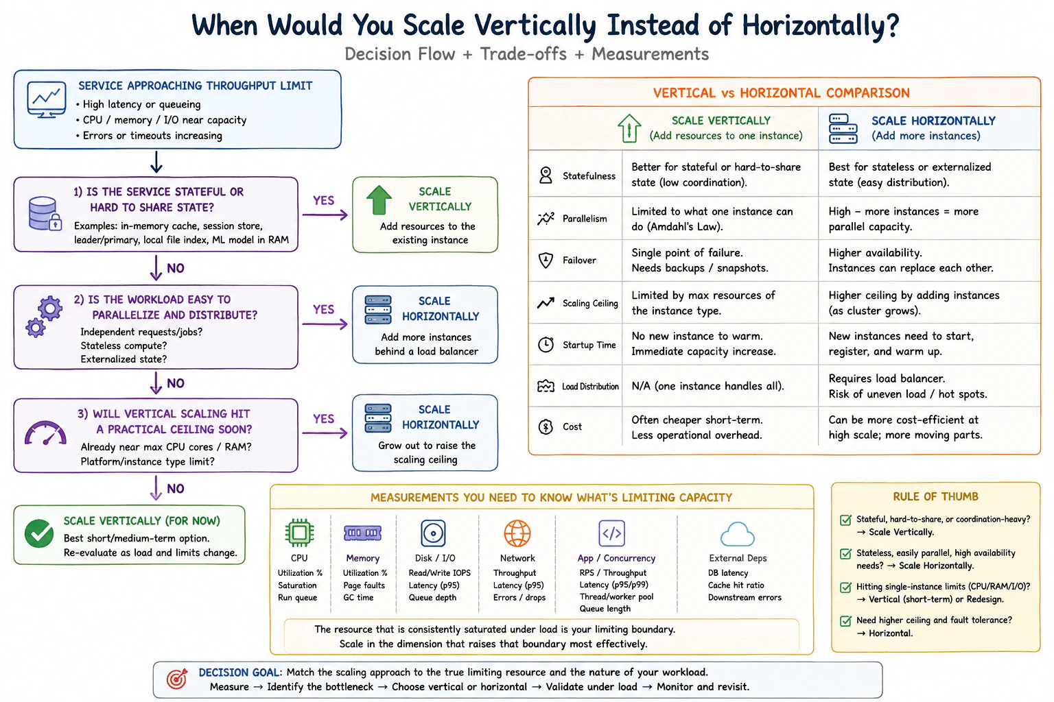
When would you scale vertically instead of horizontally? diagram
How to Explain It in an Interview

I start with measurements instead of choosing vertical or horizontal scaling from intuition. For a service approaching its current throughput limit, I reproduce or observe representative load and record throughput, latency percentiles, errors, and queueing. I then look for the resource that remains saturated as throughput stops increasing. That resource is the current capacity boundary.

I check the same measurement areas shown in the diagram. For CPU, I look at utilization, saturation, and run queue. For memory, I look at utilization, page faults, and garbage collection time when the runtime uses garbage collection. For disk input and output, I look at read and write operations, latency, and queue depth. For the network, I look at throughput, latency, errors, and drops. For the application, I look at requests per second, total throughput, latency percentiles, worker or thread pool pressure, and queue length. For external dependencies, I look at database latency, cache behavior when a cache exists, and downstream errors. I use application metrics, platform metrics, logs, and tracing only as needed to establish which boundary is actually limiting capacity.

Vertical scaling means adding resources to the existing instance. I prefer it when important state is tied to one instance or is difficult to share safely. Examples include an in memory cache, session state, a leader or primary role, a local file index, or a large model held in memory. It is also attractive when the workload has limited parallelism, because adding more instances may not create much useful parallel capacity. The amount of benefit is still limited by the work that can actually use the added resources.

Vertical scaling is operationally simpler because there is still one service instance handling the work and no new load distribution path is required. It can also provide capacity without waiting for an additional instance to register and warm. However, changing the size of an existing instance may require a restart or replacement on some platforms, so I would verify the real startup behavior instead of assuming zero interruption. The main disadvantages are the scaling ceiling and failure concentration. One instance can only grow to the largest practical instance type, and that instance remains an important failure point. I therefore still need backups, snapshots when appropriate, recovery procedures, and a failover plan.

Horizontal scaling means adding more service instances and distributing work among them. It fits best when the service is stateless or its state is externalized, and when requests or jobs can run independently. A load balancer or another distribution mechanism is normally required. I would watch for uneven load and hot spots because adding instances does not help if traffic is not distributed well.

Horizontal scaling usually gives a higher scaling ceiling because more instances can be added as demand grows. It can also improve availability because healthy instances can continue serving traffic when another instance fails. That benefit depends on correct failure detection, routing, shared dependency capacity, and placement across suitable failure domains. New instances also need time to start, register, become ready, and sometimes warm caches or other local state.

Cost depends on the workload and platform. Vertical scaling is often cheaper in the short term because there are fewer moving parts and less operational overhead. Horizontal scaling can become more cost effective at larger scale when the workload is highly parallel, but it adds costs for extra instances, load distribution, connections, shared state, monitoring, and coordination. I would compare total cost at the throughput level I actually need rather than assuming either method is always cheaper.

The final decision follows the measured boundary. If the service is stateful, hard to distribute, or limited by work that does not parallelize well, and the current instance still has useful room to grow, I would usually scale vertically. If the service is stateless, easy to parallelize, needs a higher ceiling, or needs stronger fault tolerance, I would usually scale horizontally. If the service is reaching the practical maximum size of one instance, vertical scaling may only be a short term option before horizontal scaling or redesign becomes necessary.

After the change, I rerun the same representative load. I compare throughput, latency percentiles, error rate, CPU, memory, disk, network, application concurrency, and dependency saturation. I verify that responses and service behavior remain correct. I also check whether the original bottleneck was reduced or simply moved to a database, network path, worker pool, disk path, or another dependency. I continue monitoring the same signals after deployment.

Technical Approach
  1. Define the symptom. Confirm that the service is approaching its throughput limit and record throughput, latency percentiles, errors, and queueing when present.
  2. Capture a baseline with representative load. Keep the traffic mix, request sizes, data volume, dependency behavior, and warmup conditions consistent.
  3. Identify the limiting resource. Measure CPU utilization and run queue, memory utilization and pressure, disk input and output operations and latency, network throughput and latency, application concurrency and queue length, and external dependency latency and errors.
  4. Check statefulness. If important state is tied to one instance and is difficult to share safely, vertical scaling becomes more attractive because it avoids immediate state distribution and coordination.
  5. Check parallelism. If independent requests or jobs can be distributed and state is stateless or externalized, horizontal scaling becomes more attractive. If the work has limited parallelism, more instances may provide little extra throughput.
  6. Check the scaling ceiling. If the current instance is already near the largest practical CPU, memory, or input and output capacity, horizontal scaling or redesign may be required. If useful room remains, vertical scaling can be a good short term choice.
  7. Check failover requirements. A single larger instance concentrates failure impact, while multiple correctly designed instances can provide better availability.
  8. Check startup behavior. Vertical scaling avoids starting an additional service instance, while horizontal scaling must account for instance startup, registration, readiness, and warmup.
  9. Check load distribution. Horizontal scaling requires a load balancer or another mechanism that distributes work without creating hot spots.
  10. Compare total cost. Include compute price, load distribution, extra connections, state coordination, monitoring, and operational work.
  11. Apply the chosen scaling change and rerun the same representative load.
  12. Compare the same metrics, verify correctness, and confirm that the capacity boundary improved instead of moving to another resource or dependency.
Practical Insights

Vertical scaling is usually simpler to operate because one instance continues to handle the service, but the instance can become expensive and eventually reaches a fixed maximum size. It also concentrates more failure impact in one place. Horizontal scaling adds instances, so it adds startup, warmup, load distribution, connections, shared state, coordination, monitoring, and failure handling. It can provide much more total capacity when the workload can use parallel instances effectively. Representative load testing also consumes compute and dependency capacity, but that measurement cost is necessary because scaling the wrong resource may add expense without increasing throughput.

Why Interviewers Ask This

Interviewers ask this to see whether I measure the real capacity limit before choosing a scaling method. They want to know if I understand how state, parallel work, failover, startup time, traffic distribution, cost, and the maximum size of one instance affect the decision. They also want evidence that I can validate the choice with throughput, latency, errors, and resource saturation instead of assuming that a larger instance or more instances will automatically help.

Common interview mistakes
  1. Choosing a scaling method before measuring which resource is limiting throughput.
  2. Looking only at CPU and ignoring memory pressure, disk input and output, network saturation, application concurrency, queues, locks, worker pool pressure, or external dependencies.
  3. Assuming a stateful service can be copied across instances without dealing with state ownership, consistency, and coordination.
  4. Assuming more instances always increase throughput when the workload has limited parallelism or a shared dependency is already saturated.
  5. Assuming a larger instance removes the need for failover, backups, snapshots, and recovery planning.
  6. Ignoring the fixed maximum size of one instance.
  7. Ignoring startup, readiness, registration, warmup, load balancing, and hot spots when scaling horizontally.
  8. Assuming vertical scaling always gives an immediate interruption free change without checking the platform resize behavior.
  9. Comparing only instance prices instead of total operational and dependency cost.
  10. Comparing before and after results with different workloads.
  11. Declaring success without checking correctness and whether the bottleneck moved to another resource or dependency.
Interview tip

Lead with measurement. Explain that you first identify the saturated resource, then connect the scaling choice to statefulness, parallelism, failover, scaling ceiling, startup time, load distribution, and cost. Say that vertical scaling is usually simpler but has a hard ceiling and stronger failure concentration. Say that horizontal scaling provides a higher ceiling and better fault tolerance when the work can be distributed correctly. Finish by saying that you validate the choice with the same representative load and the same metrics.
Interviewer may ask next
What if CPU is low but throughput has stopped increasing?

I would not assume that a larger CPU or more instances will help. For this service, I would keep the measurement boundary around the full request path and check memory pressure, disk latency, network saturation, worker or thread pool queueing, locks, database latency, cache behavior when relevant, and other external dependencies. A shared dependency may be the real capacity boundary. If that dependency is already saturated, adding instances can increase contention instead of throughput. The important tradeoff is that the scaling direction must follow the measured bottleneck rather than the easiest resource to resize.

What changes if the service needs better failover as well as more throughput?

Horizontal scaling becomes more attractive when this service can run correctly on multiple instances. I would externalize or safely coordinate state, distribute traffic through a load balancer or another suitable mechanism, and place instances across appropriate failure domains. I would then test both representative load and instance failure. The tradeoff is more operational complexity because startup, readiness, warmup, traffic distribution, shared dependency capacity, and state coordination must all work correctly. A vertically scaled instance can increase capacity, but by itself it does not remove the single instance failure concentration.

92. Use Little’s Law to estimate in-flight requests at 22,200 requests per second and 120 milliseconds average latency.Performance And CapacityMedium

Question Details

Treat the workload as stable over the measurement interval and convert latency to seconds before applying concurrency = throughput × latency. Calculate the expected average number of in-flight requests, then explain how that estimate informs worker, connection, and queue capacity, and why tail latency or an unstable arrival rate requires additional evidence.

Short Interview Answer (30-60 seconds)

I would first convert 120 milliseconds to 0.12 seconds. Then I apply Little's Law: average concurrency equals throughput times average latency. So 22,200 requests per second times 0.12 seconds gives about 2,664 average requests in flight. I use 2,664 as a capacity baseline, not as a direct worker count, connection pool size, or queue size. I size those resources from their measured behavior and limits, then validate p95 and p99 latency, queue depth, observed concurrency, saturation, and bursty traffic.

Detailed Explanation

The service receives 22,200 requests each second, and each request takes 120 milliseconds on average from entering the measured service path until it finishes. The goal is to estimate how many requests are present at the same time. First, change 120 milliseconds into 0.12 seconds. Multiplying 22,200 by 0.12 gives 2,664. This means about 2,664 requests are present on average while they are either waiting or being handled. This number helps with planning, but it does not directly tell us how many workers, connections, or waiting spaces we need.

Useful Questions to Ask the Interviewer
  1. Does the 120 millisecond average include both queue waiting time and service time?
  2. Is 22,200 requests per second stable over the measurement interval, or does traffic arrive in bursts?
  3. Do we have p95 and p99 latency, observed concurrency, queue depth, and saturation data?
  4. Are there known limits on worker concurrency or downstream connection pools?
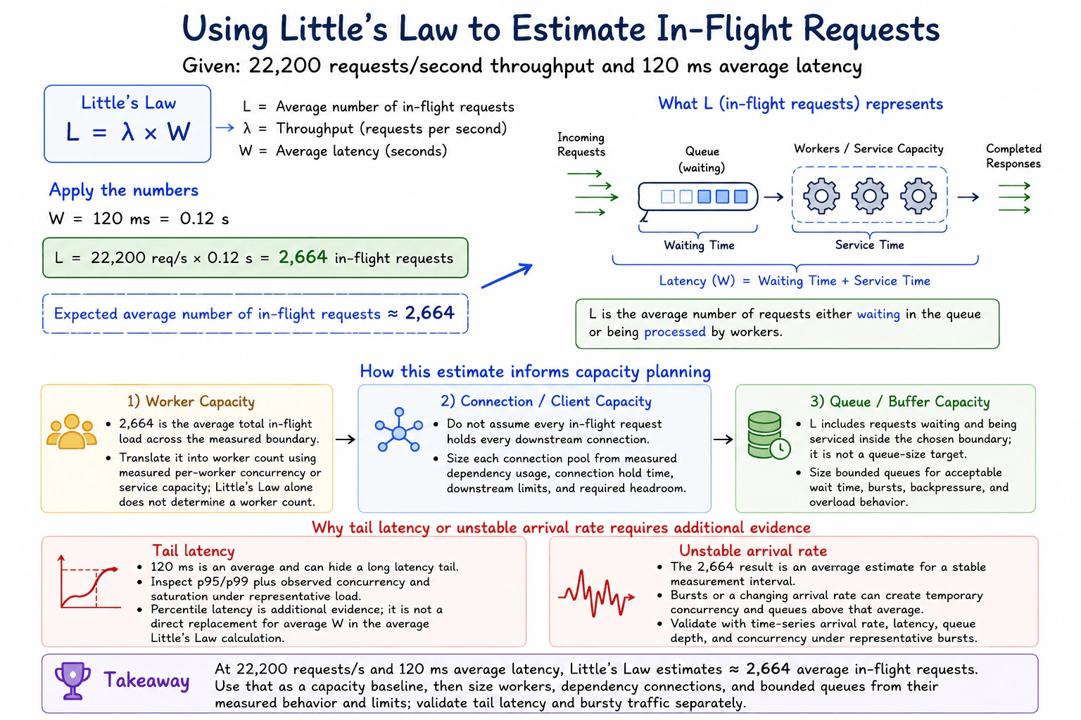
Use Little’s Law to estimate in-flight requests at 22,200 requests per second and 120 milliseconds average latency. diagram
How to Explain It in an Interview

I would define the measurement boundary first. In the diagram, a request enters the service boundary, may wait in a queue, is processed by service workers, and then completes. The 120 millisecond value represents average time across that chosen boundary, including waiting time plus service time when both are inside the measurement.

Little's Law is L = lambda times W. L is the average number of requests in the measured system. Lambda is throughput, which is 22,200 requests per second. W is average time in the system, which is 120 milliseconds or 0.12 seconds. Therefore L = 22,200 times 0.12 = 2,664. I would expect about 2,664 requests to be in flight on average during a stable measurement interval.

For worker capacity, I would not say that Little's Law tells me exactly how many workers to create. The 2,664 value is the average total load across the boundary. To turn that into a worker count, I need measured per worker concurrency or measured service capacity, plus CPU, memory, scheduling, and saturation evidence.

For connection capacity, I would not assume that every one of the 2,664 requests holds a database or other downstream connection for its entire lifetime. I would measure how often each dependency is used, how long its connection is held, the dependency limits, connection pool waiting, and the required operating margin. Each connection pool should be sized from that evidence rather than simply being set to 2,664.

For queue capacity, 2,664 is also not a queue size target. L can include requests that are waiting as well as requests currently being serviced. A bounded queue should instead be sized from acceptable waiting time, traffic bursts, backpressure behavior, overload handling, and the service rate.

The stable workload assumption matters. Little's Law gives an average relationship over a suitable measurement interval. If the arrival rate changes quickly, short bursts can create temporary concurrency and queue depth above 2,664. I would inspect time series data for arrival rate, latency, queue depth, concurrency, and saturation under representative bursts.

The average latency can also hide a long tail. A 120 millisecond average does not show whether a smaller group of requests takes much longer. I would inspect p95 and p99 latency together with observed concurrency and saturation under representative load. I would not substitute p99 directly for average W and call the result the new average concurrency. Percentile latency is additional evidence about the tail, while Little's Law uses the appropriate average time for the average relationship.

Finally, I would validate the estimate under representative traffic. I would compare throughput, average latency, p95 and p99 latency, observed concurrency, queue depth, worker saturation, connection pool waiting, errors, CPU, and memory where relevant. The practical conclusion is about 2,664 average requests in flight, with worker, connection, and bounded queue limits chosen from measured resource behavior rather than from that number alone.

Technical Approach
  1. Define the measurement boundary from request arrival through queue waiting and service processing to completion.
  2. Confirm that the workload is reasonably stable over the interval being analyzed.
  3. Convert 120 milliseconds to seconds. The result is 0.12 seconds.
  4. Apply Little's Law using L = lambda times W.
  5. Calculate 22,200 times 0.12 to get 2,664 average requests in flight.
  6. Treat 2,664 as an average capacity baseline, not as a direct worker, connection, or queue setting.
  7. Size workers using measured per worker concurrency, service capacity, CPU, memory, and saturation.
  8. Size each downstream connection pool using measured dependency usage, connection hold time, pool waiting, downstream limits, and operating margin.
  9. Size bounded queues using acceptable waiting time, burst behavior, backpressure, and overload handling.
  10. Validate with representative traffic using average latency, p95 and p99 latency, arrival rate, observed concurrency, queue depth, saturation, and error measurements.
Practical Insights

The calculation itself is constant work and uses almost no CPU or memory. The real cost comes from collecting enough production evidence to turn the estimate into safe capacity settings. More worker concurrency can consume more CPU and memory. Larger connection pools can put more pressure on downstream systems. Larger queues can consume memory and increase waiting time. Representative load tests also use time and infrastructure. The goal is to use the 2,664 estimate as a starting point and add only the capacity supported by measurements.

Why Interviewers Ask This

Interviewers ask this to check whether a candidate can turn request rate and response time into a useful capacity estimate without treating that estimate as an exact worker, connection, or queue requirement. They also want to see whether the candidate understands measurement boundaries, averages, traffic stability, tail latency, downstream limits, bounded queues, and the need to validate capacity with representative production behavior.

Common interview mistakes

Common mistakes include forgetting to convert 120 milliseconds to 0.12 seconds, treating 2,664 as an exact maximum instead of an average, assuming that every request holds a downstream connection for its entire lifetime, and setting every connection pool to 2,664. Another mistake is treating 2,664 as the required queue size even though the measured number can include both waiting and active requests. Candidates may also ignore bursty arrivals, use only average latency, substitute p99 directly for average W, create unbounded queues or concurrency, or size capacity without checking worker saturation, dependency limits, queue waiting, CPU, memory, and errors.

Interview tip

State the arithmetic first: 120 milliseconds is 0.12 seconds, so 22,200 times 0.12 equals 2,664 average requests in flight. Then immediately explain the important limit: 2,664 is a capacity baseline, not a direct worker count, connection pool size, or queue size. Finish by saying that you would validate tail latency, bursts, observed concurrency, queue depth, saturation, and downstream limits under representative load.

Interviewer may ask next
What if the average latency is still 120 milliseconds, but p99 latency is much higher?

I would keep 2,664 as the average Little's Law estimate for the measured request boundary because it comes from the average latency of 0.12 seconds. A much higher p99 tells me that some requests remain in the system much longer than the average, so the average alone may hide periods of high concurrency or saturation. I would inspect p95 and p99 latency together with observed concurrency, queue depth, worker saturation, connection pool waiting, and errors under representative load. I would not substitute p99 directly for average W and describe that result as average concurrency.

How would you use the 2,664 estimate if traffic arrives in short bursts instead of at a stable rate?

I would use 2,664 only as the average baseline for the measured service boundary, not as the required peak capacity. Bursty arrival rates can temporarily push concurrency and queue depth above that value. I would collect time series measurements for arrival rate, latency, observed concurrency, queue depth, worker saturation, connection usage, and errors during representative bursts. Worker limits, connection pools, and bounded queues would then be chosen from those measured peak behaviors and downstream limits, with backpressure and overload handling included so a burst cannot create unbounded resource growth.

93. How would you locate the bottleneck in a slow request path?Performance And CapacityMedium

Question Details

A request crosses a load balancer, application workers, a connection pool, a database, and a downstream API. Latency percentiles, throughput, errors, CPU, memory, queue depth, pool wait time, disk and network data, and traces are available. Build a measurement sequence that identifies the first saturated boundary, validates causality under load, and rules out merely correlated utilization.

Short Interview Answer (30-60 seconds)

I would first establish a baseline for latency percentiles, throughput, errors, and saturation across the request path. Then I would use traces to split total latency across the load balancer, application workers, connection pool, database, and downstream API. I would increase representative load in small steps and watch for the first boundary where queueing, wait time, or service time rises sharply. I would then reduce the constraint or increase safe capacity only at that boundary and repeat the same load test. If overall latency and errors improve and the queueing signal disappears, that strongly supports causality.

Detailed Explanation

The goal is to find the first place where a request begins to wait because one part of the path cannot keep up. I would watch the whole journey, from the first entry point through the workers, shared connection limit, stored data, and outside service. I would record normal response time and request volume first. Then I would add load slowly and see where waiting grows earliest. A busy part is not proof by itself. I want to see that the same place becomes constrained as demand rises and that changing it improves the whole request.

Useful Questions to Ask the Interviewer
  1. Which latency percentile matters most for this service, such as p95 or p99?
  2. Can I run a representative load test safely, or must I use production traffic only for observation?
  3. Are the traces complete enough to show timing for the application workers, database calls, and downstream API calls?
  4. Are there known limits for worker concurrency, connection pool size, database capacity, or downstream API quotas?
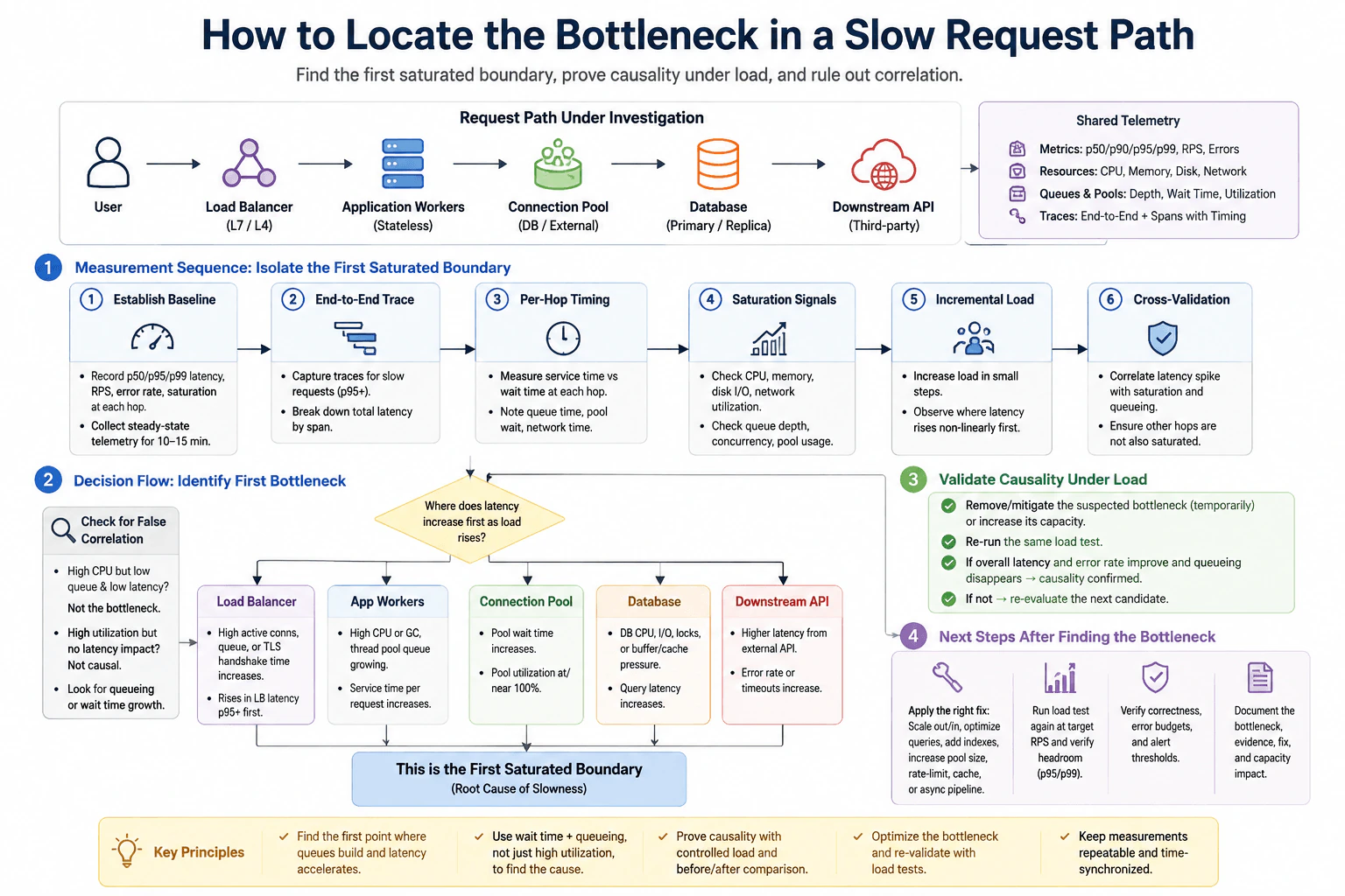
How would you locate the bottleneck in a slow request path? diagram
How to Explain It in an Interview

I would start by defining the measurable symptom. For this request path, I would record p50, p90, p95, and p99 latency, throughput, error rate, and saturation signals at steady load. The diagram also shows collecting steady state telemetry before changing anything. This gives me a baseline for comparison.

Next, I would follow the exact request path shown in the diagram: user to load balancer, stateless application workers, connection pool, database, downstream API, and then the response. I would use end to end traces to divide the total latency into spans and identify how much time is spent at each boundary. Tracing shows where time is spent. Metrics show whether a component is approaching capacity. I need both kinds of evidence.

For each hop, I would separate service time from waiting time when possible. Queue time, connection pool wait time, network wait, and dependency time matter because a request can be slow even when application execution itself is fast.

At the load balancer, I would inspect active connections, queueing, CPU when relevant, and connection or TLS handshake time when those measurements are available. I would look for increasing load balancer latency as demand rises.

At the application workers, I would inspect CPU, memory, worker availability, queue depth, service time per request, and runtime pauses or thread pool queue growth when relevant. High CPU alone is not enough. I want evidence that service time or queueing worsens as load grows.

At the connection pool, I would focus on pool wait time and pool utilization. If requests spend more time waiting to obtain a connection as load increases, the pool or the dependency using those connections becomes a strong bottleneck candidate. A highly utilized pool is not proof by itself if requests are still obtaining connections quickly.

At the database, I would compare query latency with database CPU, disk input and output, connection use, locks or transaction contention when available, and buffer or cache pressure when those measurements are available. I would not claim that an application trace alone proves a database root cause. Database specific evidence must support that conclusion.

At the downstream API, I would compare trace span latency, network data, timeout rate, error rate, and any known service limits. If the downstream call becomes slower while local application measurements remain healthy, adding local workers may only put more pressure on that external dependency.

After collecting the baseline and per hop timing, I would increase representative load in small steps. At each step I would compare latency, throughput, errors, CPU, memory, queue depth, connection pool wait time, disk input and output, network behavior, and trace timing. I am looking for the earliest boundary where demand starts exceeding useful capacity. Strong evidence includes growing queue depth or wait time, rising latency, increasing errors or timeouts, and throughput that stops growing normally.

I would then rule out false correlation. For example, application worker CPU can be high while queue depth remains low and latency stays stable. In that case the CPU is busy, but the evidence does not show that CPU is the limiting boundary. High utilization without a latency, queueing, wait time, error, or throughput effect is not enough to name the bottleneck.

Once I have the strongest candidate, I would validate causality under the same load. I would temporarily remove or reduce that constraint, or safely increase its capacity. Then I would repeat the same representative load test. If overall latency and error rate improve and the queueing or wait signal at that boundary disappears, that supports the bottleneck conclusion. If the expected improvement does not appear, I would reevaluate the next candidate rather than forcing the first theory.

The production change must target the measured bottleneck. If the database is limiting capacity, the evidence may support a query improvement, database capacity change, or another database specific correction. If the application workers are limiting capacity, the evidence may support worker capacity changes after checking CPU and memory limits. If connection pool wait is the first saturation signal, pool tuning may help only when the database can safely accept the additional connections. If the downstream API is limiting the path, the solution may instead involve fewer calls, caching when correctness permits it, rate control, or another dependency specific change.

After the targeted change, I would run the same representative workload again and compare the same p95 and p99 latency, throughput, error rate, worker headroom, queueing, pool wait time, resource measurements, and dependency timing. I would verify that responses are still correct. I would also check whether the bottleneck moved to another resource or dependency. Finally, I would keep the same measurements and traces in production so the new capacity limit can be detected.

Technical Approach
  1. Define the slow request and choose the main success measurements, especially p95 or p99 latency, throughput, and error rate.
  2. Capture a steady load baseline across the complete request path.
  3. Use traces to split end to end latency across the load balancer, application workers, connection pool, database, and downstream API.
  4. Measure service time and waiting time at each hop. Include queue time, connection pool wait time, and network or dependency time when available.
  5. Compare CPU, memory, queue depth, pool wait time, disk input and output, network data, errors, and trace timing.
  6. Increase representative load in small steps and watch for the earliest boundary where wait time or queue depth grows, latency rises sharply, errors appear, or useful throughput stops increasing normally.
  7. Rule out simple correlation. High utilization without increasing latency, waiting, queueing, errors, or reduced throughput is not enough to identify a bottleneck.
  8. Select the strongest candidate for the first saturated boundary.
  9. Temporarily reduce its work, remove its constraint, or increase its safe capacity.
  10. Repeat the same load test. If overall latency and errors improve and the saturation signal at that boundary falls, the experiment supports causality.
  11. Apply one targeted production change that addresses the measured constraint.
  12. Retest with the same traffic mix, concurrency, payloads, data, and dependency behavior.
  13. Verify correctness and check whether the bottleneck moved to another boundary.
  14. Continue monitoring the same measurements and traces after deployment.
Practical Insights

The main cost is measurement and controlled testing rather than algorithmic complexity. First level metrics are usually relatively low cost. Tracing adds instrumentation, processing, and storage cost and can be sampled, so it may not capture every request. Representative load tests consume real worker, database, connection, disk, network, and downstream capacity, so the test must be bounded and planned carefully. Increasing workers or connection capacity can also increase CPU, memory, database pressure, and downstream traffic. The safest approach is to increase load in small steps and compare the same measurements before and after each change.

Why Interviewers Ask This

Interviewers ask this to see whether I diagnose performance problems from measurements instead of guessing. They want to know whether I can follow latency across the load balancer, application workers, connection pool, database, and downstream API, identify the first saturated boundary, distinguish service time from waiting time, and prove that a suspected resource is causing the slowdown rather than merely being busy at the same time.

Common interview mistakes

Common mistakes include optimizing before recording a baseline, using only average latency, blaming the component with the highest utilization, and treating high CPU as proof of a CPU bottleneck. Another mistake is looking only at application execution while ignoring queue depth, connection pool wait time, database latency, disk input and output, network latency, or the downstream API. Increasing workers or pool size without checking the next dependency can move the bottleneck instead of removing it. A single trace or one local test is not proof. Before and after tests must use the same representative workload, and the final check must verify correctness.

Interview tip

Explain the investigation as an evidence sequence. Start with the baseline, trace the complete request, measure service time and waiting time, identify where queueing or latency first grows under load, and then prove causality with the same load before and after a targeted change. Emphasize that high utilization alone does not prove a bottleneck.

Interviewer may ask next
What if application worker CPU is very high, but queue depth and request latency do not increase as load rises?

I would not call the application workers the bottleneck from CPU utilization alone. For this exact request path, I would keep measuring the load balancer, application workers, connection pool, database, and downstream API while increasing the same representative load. If worker queue depth stays low, service time remains stable, throughput continues to grow, and p95 or p99 latency does not worsen, the high CPU can be correlated utilization rather than the first saturated boundary. I would look for the earliest place where waiting, queueing, errors, or latency actually grows. The tradeoff is that high CPU still reduces headroom for bursts, so I would continue monitoring it even when it is not the current cause.

What would you do if increasing connection pool capacity removes pool wait time but database latency then rises sharply?

I would treat that as evidence that the bottleneck moved from the connection pool boundary to the database boundary. For the same request path, I would repeat the representative load while comparing pool wait time, database call latency, database CPU, disk input and output, connection use, errors, and trace spans. I would not keep increasing the pool because more connections can place more pressure on the database. I would investigate the measured database constraint and choose a database specific change only when the evidence supports it. After that change, I would run the same workload again and verify latency, throughput, errors, correctness, and the new saturation point.

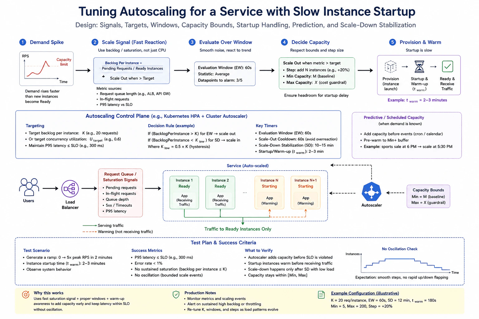
94. How would you tune autoscaling for a service with slow instance startup?Performance And CapacityMedium

Question Details

Demand changes faster than new instances become Ready. Design a scaling signal, target, evaluation window, minimum and maximum capacity, startup and warm-up handling, predictive or scheduled capacity where justified, scale-down stabilization, and a test that proves the latency objective is maintained without oscillation.

Short Interview Answer (30-60 seconds)

I would scale from a fast demand or saturation signal such as backlog per Ready instance, with p95 latency as a guardrail, instead of relying only on CPU. I would measure startup and warmup time, choose a target and evaluation window that react early enough, keep enough minimum capacity for normal demand, and set a maximum for cost and quota protection. New instances would receive traffic only after they are Ready and warmed. For predictable peaks I would add capacity before demand arrives. I would use a longer scale down stabilization window and validate the policy with repeated load spikes while checking p95 latency and scaling events for oscillation.

Detailed Explanation

The problem is that customer demand can rise before new service instances are ready to help. If scaling starts too late, requests wait and response time gets worse. I would watch demand early, keep spare capacity, and measure how long a new instance needs before it can safely serve traffic. I would also avoid removing capacity too quickly after traffic falls. Finally, I would test sudden and repeated demand changes and confirm that response time stays within the required goal without the service repeatedly adding and removing instances.

Useful Questions to Ask the Interviewer
  1. How long does an instance normally take from creation until it is Ready and fully warmed?
  2. Is the workload driven mainly by request rate, queue depth, in flight requests, or another demand signal?
  3. What p95 latency objective and error rate must the service maintain?
  4. Are there predictable traffic peaks where scheduled or predictive capacity is justified?
  5. What cost, quota, or downstream limits should define minimum and maximum capacity?
How would you tune autoscaling for a service with slow instance startup? diagram
How to Explain It in an Interview

I would first measure the total delay from instance creation until useful serving capacity exists. That includes startup time, the readiness transition, and any additional warmup needed before performance becomes stable. The autoscaling policy must react early enough to cover this delay.

For the scaling signal, I would prefer a demand or saturation metric that increases before overloaded instances produce severe latency. The diagram uses backlog per Ready instance as the main signal. It is calculated from pending requests divided by the number of Ready instances. Request queue length, in flight requests, and p95 latency are supporting signals. CPU can still be monitored, but I would not depend on CPU alone when demand grows faster than capacity can start.

I would set a target for backlog per Ready instance based on measured steady state capacity. The diagram gives an illustrative value of about 20 requests per instance. Another possible target shown in the diagram is concurrency utilization. P95 latency remains a guardrail so the control policy stays connected to the user visible objective.

I would evaluate the signal over a short window that smooths brief noise but still reacts before the startup delay causes an SLO violation. The diagram uses an illustrative 60 second evaluation window and shows an example where several datapoints must indicate sustained pressure before scale out. The exact window should be tuned from real traffic patterns and measured startup behavior.

I would set minimum capacity high enough for normal traffic plus useful headroom while new instances start. The diagram shows an illustrative minimum of 5. I would set maximum capacity from cost, quota, downstream connection limits, and other service constraints. The diagram shows an illustrative maximum of 200. These values are examples rather than universal settings.

When the scaling metric remains above its target, I would scale out in a meaningful step rather than adding one instance too slowly during a fast spike. The diagram shows an illustrative increase of about 20 percent. The actual step should come from the demand growth rate, safe throughput per Ready instance, and measured startup delay.

Starting instances must not be treated as useful serving capacity too early. The diagram separates Ready instances from Starting instances and shows that traffic is sent only to Ready instances. A new instance should complete its startup checks and any required warmup before it is relied on for serving traffic. The diagram gives an illustrative warmup duration of roughly two to three minutes.

If demand is predictable, I would use scheduled or predictive capacity to start instances before the expected spike. The diagram gives the example of an event at 6 PM with capacity added around 5:30 PM. The real lead time should be based on measured startup and warmup behavior plus a safety buffer.

Scale down should be deliberately slower than scale out. I would use hysteresis, which means using a lower threshold for scaling in than for scaling out, plus a stabilization window so a brief traffic drop does not immediately remove capacity. The diagram shows an illustrative low threshold around half the scale out target and a stabilization period of roughly 10 to 15 minutes. Capacity can then be reduced gradually while never going below the configured minimum.

To verify the policy, I would use a representative load test with the same traffic shape and instance startup behavior expected in production. The diagram shows an illustrative ramp from normal traffic to about five times peak request rate over two minutes. I would also test repeated spikes and drops because a single increase cannot prove that the control loop is stable. I would record p95 latency, errors, backlog or saturation, Ready and Starting instance counts, total capacity, and every scaling event.

The policy passes when p95 latency stays within its SLO, errors remain within the accepted target, backlog does not remain saturated, new instances are warmed before they are relied on for traffic, capacity remains between minimum and maximum bounds, and scaling events do not repeatedly reverse direction. I would monitor the same signals in production and adjust the target, evaluation window, capacity step, minimum capacity, and stabilization time if real traffic behaves differently.

Technical Approach
  1. Measure the full delay from instance creation through readiness and warmup.
  2. Measure steady state request capacity per Ready instance under representative load.
  3. Choose a fast demand or saturation signal such as backlog per Ready instance, with p95 latency as a user impact guardrail.
  4. Set the target from measured safe capacity rather than from a guessed percentage.
  5. Choose an evaluation window that filters brief noise but still reacts early enough for the measured startup delay.
  6. Set minimum capacity to cover baseline demand plus useful startup headroom.
  7. Set maximum capacity from cost, platform quota, downstream capacity, and operational limits.
  8. Scale out in steps large enough to respond to the observed demand growth rate.
  9. Keep Starting instances out of effective serving capacity until they are Ready and any required warmup is complete.
  10. Add scheduled or predictive capacity before known peaks when demand is sufficiently predictable.
  11. Use a lower scale in threshold than the scale out threshold and apply a longer stabilization window after demand falls.
  12. Reduce capacity gradually and never below minimum capacity.
  13. Test sudden ramps, drops, and repeated spikes with representative traffic.
  14. Verify p95 latency, errors, backlog, instance state transitions, capacity bounds, and scaling event frequency.
  15. Monitor the same signals in production and retune the policy when measured workload behavior changes.
Practical Insights

The main cost is spare capacity. Keeping a higher minimum gives the service more time to absorb a spike, but it costs more while traffic is low. Larger scale out steps react faster, but they can create unnecessary instances when the signal is noisy. A short evaluation window reacts quickly but may respond to temporary variation. A longer window is smoother but may react too late. Startup and warmup consume CPU, memory, image download bandwidth, connections, and platform capacity before the new instance becomes useful. Scheduled or predictive scaling also adds maintenance because forecasts and schedules must remain accurate. A longer scale down stabilization window keeps extra instances for a while after traffic falls, which costs more but reduces repeated removal and recreation of capacity.

Why Interviewers Ask This

Interviewers ask this to see whether I understand autoscaling as a control problem with delayed capacity. They want to know whether I can choose a demand signal that reacts before latency becomes bad, set useful minimum and maximum capacity, account for startup and warmup time, prevent repeated scaling in and out, and prove the result with representative load. They are also checking whether I understand that CPU alone may react too late when demand rises faster than new instances become Ready.

Common interview mistakes

A common mistake is scaling only from CPU even though request backlog or concurrency increases earlier. Another mistake is counting Starting instances as available capacity before they can safely serve traffic. Setting minimum capacity too low can leave the service unable to absorb demand during startup delay. Setting maximum capacity without considering quotas or downstream limits can move saturation to another dependency. An evaluation window that is too long can delay scale out, while one that is too short can react to noise. Scaling down immediately after a traffic drop can cause repeated removal and creation of instances. Another mistake is copying example values such as 60 seconds, 20 percent, or 10 to 15 minutes without measuring the workload. Finally, testing only one smooth traffic ramp can hide oscillation that appears during repeated spikes and drops.

Interview tip

Explain autoscaling as a delayed control loop. Start with the demand signal, then describe the target, evaluation window, startup delay, capacity bounds, warmup handling, predictive capacity when justified, and slower scale down. Make it clear that the exact numbers come from measurement. Finish by explaining how repeated representative load tests prove both the latency objective and stable scaling behavior.

Interviewer may ask next
What if CPU stays low while p95 latency and request backlog keep rising?

I would not conclude that CPU capacity is the problem. For this slow startup service, the measurement boundary includes request backlog, in flight requests, p95 latency, Ready instance count, and dependency behavior. Rising backlog with low CPU can mean requests are waiting on a database, network service, connection pool, lock, or another constrained resource. I would use service metrics and request timing evidence to find where the waiting occurs. I would still use a demand or saturation signal for autoscaling when it represents real pressure, but I would not let additional replicas hide a shared downstream bottleneck. The main tradeoff is that more replicas may reduce local queue pressure only until the shared dependency reaches its own limit.

How would you roll out a more aggressive scale out policy without causing instability or excessive cost?

I would change the policy gradually and compare the same service metrics before expanding it. For this workload, I would watch backlog per Ready instance, p95 latency, errors, Ready and Starting instance counts, startup and warmup time, total capacity, and scaling events. I would compare the new target, evaluation window, or scale out step with the previous settings under the same representative traffic pattern. In production I would watch for unnecessary capacity growth, quota pressure, downstream saturation, and repeated scaling reversals. A more aggressive policy can protect latency earlier, but it may increase cost and pressure shared dependencies, so minimum and maximum capacity plus downstream limits remain important guardrails.

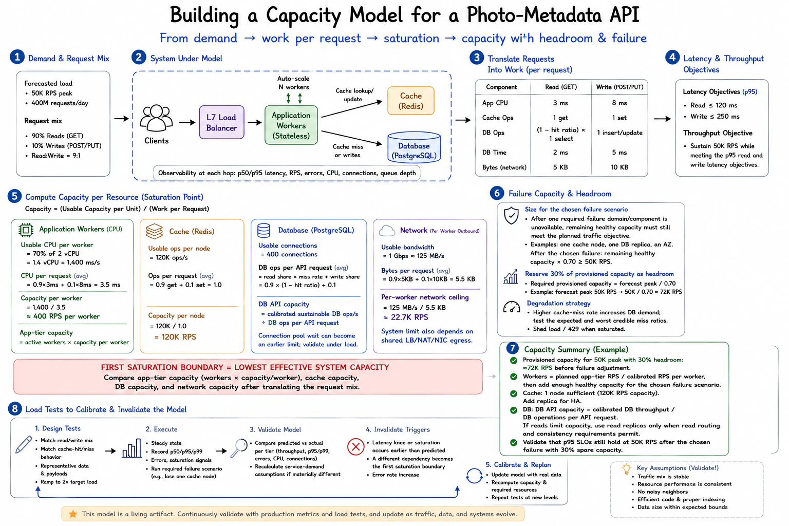
95. How would you build a capacity model for a photo-metadata API?Performance And CapacityHard

Question Details

The service receives metadata reads and writes and depends on application workers, a cache, and a database. Start from demand and request mix, translate each request into work at every dependency, set latency and throughput objectives, identify the first saturation boundary, include failure capacity and headroom, and define load tests that can calibrate and invalidate the model.

Short Interview Answer (30-60 seconds)

I would start with forecast demand and the read and write mix, then translate one API request into work at the application workers, cache, database, and network. I would measure sustainable capacity for each resource while the latency objectives still hold. The first saturation boundary is the lowest effective system capacity after applying the real request mix. I would then reserve headroom, verify that enough healthy capacity remains during the chosen failure scenario, and run representative load tests to compare predicted and observed latency, throughput, errors, connections, and saturation. If measurements disagree with the model, I would update the assumptions and calculate capacity again.

Detailed Explanation

A capacity model tells us how much traffic the photo metadata service can safely handle. I would first estimate how many requests arrive and how many are reads or writes. Then I would work out how much application, cache, database, and network work each request creates. I would compare those needs with the measured capacity of each part. The smallest safe capacity becomes the first limit. I would leave spare capacity for traffic changes and failures. Finally, I would test the service with realistic traffic and update the model whenever measured results differ from the prediction.

Useful Questions to Ask the Interviewer
  1. What peak and normal request rates should the service support?
  2. What percentage of requests are reads and what percentage are writes?
  3. What cache hit ratio should I expect during normal traffic and during cache disruption?
  4. What p95 latency objectives should reads and writes meet?
  5. Which failure scenario must the service continue to handle, such as losing a cache node, database replica, or availability zone?
  6. Should the model include a required amount of spare capacity at peak traffic?
How would you build a capacity model for a photo-metadata API? diagram
How to Explain It in an Interview

I would begin with demand. In the diagram example, the forecast peak is 50K RPS and the service receives about 90% reads and 10% writes. I would not size the system from total RPS alone because reads and writes create different amounts of application, cache, database, and network work.

Next I would define the measurement boundary. Requests enter through the load balancer and reach stateless application workers. The application then calls Redis and PostgreSQL as needed. The application owns both dependency calls. Redis does not call PostgreSQL. A read performs one cache get. Only a cache miss creates the database read. A write creates one database insert or update and a separate cache operation according to the cache policy.

I would then translate the request mix into work. The diagram uses an illustrative application CPU cost of about 3 ms for a read and 8 ms for a write. With the 90 to 10 mix, average application CPU demand is about 3.5 ms per API request. If one worker has about 1400 ms of usable CPU time each second, the illustrative capacity is about 400 RPS per worker. Total application tier capacity is the number of active workers multiplied by calibrated capacity per worker.

For Redis, I would measure sustainable cache operations per second while the required latency still holds. The diagram has one cache operation per API request on average. A cache node calibrated at 120K operations per second therefore represents about 120K API requests per second for that request mix. I would still test realistic cache hit and miss behavior because a higher miss ratio moves more read traffic to PostgreSQL.

For PostgreSQL, I would calculate database operations per API request as read share multiplied by cache miss ratio, plus write share. In the diagram that is 0.9 multiplied by one minus the cache hit ratio, plus 0.1. I would then divide calibrated sustainable database operations per second by database operations per API request to estimate the API capacity allowed by the database. I would treat the 400 connection pool limit separately because connection pool waiting can become an earlier saturation point even when raw database throughput has not reached its limit.

For network capacity, I would translate average bytes per API request into bandwidth demand. The diagram uses about 5.5 KB per API request and about 125 MB per second of usable outbound bandwidth for one worker. That gives an illustrative per worker network ceiling of about 22.7K RPS. I would not treat this as the complete system network capacity because shared load balancer, NAT, NIC, and other egress limits can become the real network boundary.

I would then set explicit service objectives. The diagram targets read p95 latency at or below 120 ms and write p95 latency at or below 250 ms. The throughput objective is to sustain 50K RPS while meeting those read and write latency objectives. A resource only provides usable capacity while the service remains inside those objectives.

The first saturation boundary is the lowest effective system capacity after translating the real request mix. I would compare total application tier capacity, cache capacity, database capacity, connection pool constraints, and system network capacity. I would not call one worker or one dependency the bottleneck without comparing these limits at the system level.

Next I would include headroom and failure capacity. The diagram reserves 30% of provisioned capacity as spare capacity. For a forecast peak of 50K RPS, provisioned capacity before failure adjustment is 50K divided by 0.70, which is about 72K RPS. I would then apply the chosen failure scenario. After that failure, the remaining healthy capacity multiplied by 0.70 still needs to be at least 50K RPS. That makes the failure requirement explicit instead of assuming one extra component is automatically enough.

Finally, I would calibrate and try to invalidate the model with load tests. The tests should match the read and write mix, cache hit and miss behavior, representative payloads, realistic data scale, and the required failure scenario. I would ramp traffic, hold a steady state, and record p50, p95, and p99 latency, throughput, errors, CPU, connection pressure, and saturation signals. I would compare predicted and observed results at every tier. If the latency knee appears earlier than predicted, errors rise, or another dependency becomes the first saturation boundary, I would update the service demand assumptions, recalculate capacity, and repeat the test.

The main tradeoff is cost versus safety margin. Extra workers, cache capacity, database capacity, and network capacity cost more, but running too close to saturation makes latency and recovery less predictable. More workers, cache replicas, database read replicas, or more bandwidth are not automatic fixes. I would add capacity where measurements show it is needed. If database reads become limiting, I would use read replicas only when read routing and consistency requirements permit. I would keep validating the model with production metrics and repeat load tests as traffic, data, cache behavior, and system performance change.

Technical Approach
  1. Forecast normal and peak request rates and record the read and write mix.
  2. Set the throughput objective and separate p95 latency objectives for reads and writes.
  3. Map the request path from the load balancer to stateless application workers and from the application to Redis and PostgreSQL.
  4. Translate one read and one write into application CPU time, cache operations, database operations, and network bytes.
  5. Use the traffic mix to calculate average work per API request for each resource.
  6. Measure sustainable capacity for each application worker, cache node, database, connection pool, and relevant network boundary while the latency objectives still hold.
  7. Calculate total application tier capacity as active workers multiplied by calibrated capacity per worker.
  8. Calculate database API capacity as calibrated sustainable database operations per second divided by database operations per API request. Treat connection pool waiting as a separate possible limit.
  9. Convert bytes per API request into network demand and evaluate both per worker and shared network limits.
  10. Compare effective capacities and identify the first system resource that reaches saturation.
  11. Reserve the required headroom. With 30% spare capacity, provisioned capacity for a 50K RPS peak is about 50K divided by 0.70, or about 72K RPS before failure adjustment.
  12. Apply the chosen failure scenario and verify that remaining healthy capacity multiplied by 0.70 is still at least 50K RPS.
  13. Load test with the same read and write mix, cache behavior, payloads, data scale, and failure scenario expected in production.
  14. Compare predicted and observed p95 and p99 latency, throughput, errors, CPU, connections, and saturation.
  15. If saturation happens earlier than predicted or moves to another dependency, update the model assumptions and repeat the test.
Practical Insights

The main cost is not an algorithmic Big O cost. It is the resource and operational cost of keeping enough safe capacity. More application workers consume more CPU and memory and may create more database connections. More cache capacity uses more memory and adds replication cost. Database capacity may require stronger hardware, connection tuning, or read replicas when the workload and consistency rules permit them. Extra network capacity may also be required. Reserving 30% spare capacity means paying for resources that are intentionally unused during normal peak traffic. Representative load tests also consume compute time and engineering time, but they are necessary because a paper model cannot prove real latency or saturation behavior.

Why Interviewers Ask This

Interviewers want to see whether I can turn traffic demand into measurable work across the complete service instead of guessing how many servers are needed. They are testing whether I understand request mix, application worker capacity, cache behavior, database demand, network limits, latency objectives, saturation, spare capacity, failure capacity, and realistic load testing. They also want to see whether I treat a capacity model as an estimate that must be calibrated with measurements and revised when another resource becomes the first limit.

Common interview mistakes

Common mistakes include sizing only from total RPS and ignoring the read and write mix, assuming every read reaches the database even when a cache exists, treating Redis as if it directly calls PostgreSQL, and using one worker capacity as if it were total application tier capacity. Another mistake is deriving database throughput only from connection count. Connection count is a constraint, but sustainable database operations per second must be calibrated under load. It is also wrong to attach a latency percentile directly to throughput, ignore shared network limits, or declare the first bottleneck before comparing system level capacities. Teams can also underestimate risk by reserving headroom but forgetting failure capacity, testing only normal cache behavior, using different workloads for prediction and validation, or accepting a result without checking whether the bottleneck moved to another dependency.

Interview tip

Explain the model as a chain from demand to work to capacity to saturation to validation. State the request mix first. Then show how one request consumes application, cache, database, and network resources. Make it clear that the smallest measured effective system capacity is the first saturation boundary. Finish with headroom, the required failure scenario, and a realistic load test that can prove the model wrong. This shows that capacity planning is a measurable engineering process rather than a server count guess.

Interviewer may ask next
What if the cache hit ratio falls during peak traffic and the database saturates much earlier than your model predicted?

I would treat the cache hit ratio as a model input that changed rather than assume the original database capacity is still valid. For this photo metadata API, database operations per API request equal the read share multiplied by the cache miss ratio, plus the write share. A lower hit ratio raises database demand at the same API RPS. I would reproduce the lower hit ratio under representative load, then measure database operations, query latency, connection pool wait, errors, and API p95 latency. I would recalculate database API capacity from the measured database throughput. The tradeoff is that designing for a very poor hit ratio costs more database capacity, while designing only for normal cache behavior increases risk during cache disruption.

How would you know whether adding more application workers will actually increase capacity?

I would add workers only when the application tier is the measured saturation boundary and downstream resources still have spare capacity. For this photo metadata API, total application tier capacity is active workers multiplied by calibrated RPS per worker, but that stops helping when Redis, PostgreSQL, the connection pool, or shared network capacity becomes the next limit. I would run the same representative load test before and after changing worker count and compare throughput, p95 and p99 latency, CPU, errors, connections, and dependency saturation. The tradeoff is that more workers add application capacity but can also increase database connections and downstream pressure, so the bottleneck may simply move.

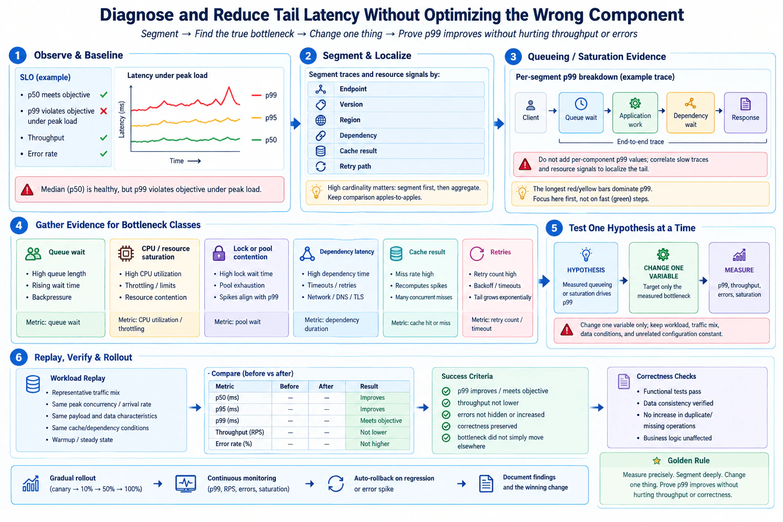
96. How would you diagnose and reduce tail latency without optimizing the wrong component?Performance And CapacityHard

Question Details

Median latency meets the objective but p99 violates it under peak load. Segment traces and resource signals by endpoint, version, region, dependency, cache result, and retry path; identify queueing and saturation; test one hypothesis at a time; and define a workload replay that proves the p99 improvement without lowering throughput or hiding errors.

Short Interview Answer (30-60 seconds)

I would start with the p99 symptom and capture a baseline under peak load. Then I would segment traces and resource signals by endpoint, version, region, dependency, cache result, and retry path. I would correlate slow traces with queue waits, CPU or resource saturation, pool contention, dependency latency, cache misses, and retries. I would change only the measured bottleneck and replay the same representative workload. I would accept the change only if p99 improves, throughput does not fall, errors are not hidden or increased, correctness is preserved, and saturation does not move somewhere else.

Detailed Explanation

The main idea is to find where the slowest requests spend their time before changing anything. Most requests may already be fast, while a small group becomes very slow during busy periods. I would compare those slow requests across different parts of the system and look for waiting, overloaded resources, slow outside calls, cache behavior, or repeated attempts. Then I would change only the part supported by evidence. Finally, I would repeat the same realistic test and confirm that speed improves without reducing useful work, hiding failures, or breaking correct behavior.

Useful Questions to Ask the Interviewer
  1. What p99 objective should the service meet during peak load?
  2. Which traffic mix and peak concurrency should the replay represent?
  3. Are traces available with endpoint, version, region, dependency, cache result, and retry information?
  4. Which resource limits and downstream capacity limits should stay constant during the test?
How would you diagnose and reduce tail latency without optimizing the wrong component? diagram
How to Explain It in an Interview

I would begin with the measurable symptom. Median latency meets the objective, but p99 becomes too slow under peak load. I would record the baseline p50, p95, p99, throughput, error rate, and relevant saturation signals before making a change.

Next, I would define the measurement boundary from request arrival through queue wait, application work, dependency wait, and response completion. I would use distributed traces to see the timing of individual slow requests. I would use service and platform metrics to see trends, resource use, throttling, and saturation. Error, timeout, and retry signals help explain whether failures or repeated work are stretching the tail.

I would then segment the evidence by endpoint, version, region, dependency, cache result, and retry path. This matters because one overall p99 can hide a bad slice. I would compare similar slices with similar slices instead of mixing unrelated traffic. I would also avoid adding separate component p99 values together. Percentiles from different components are not additive. Instead, I would inspect slow end to end traces and correlate their span timing with queue and resource signals.

The next step is bottleneck classification. High queue wait or growing queue length can indicate backlog. High CPU utilization or throttling can indicate resource saturation. High lock wait or pool wait can indicate contention. High dependency duration can indicate an outside service or network path is dominating the tail. A high cache miss rate can increase dependency work. Retries and backoff can amplify latency when a dependency is already struggling.

I would form one hypothesis from the strongest correlated evidence. For example, the hypothesis might be that measured queueing or resource saturation is driving p99. I would then change one variable that targets only that measured bottleneck. I would keep the workload, traffic mix, data conditions, cache and dependency conditions, and unrelated configuration constant so the result can be attributed to that change.

To prove the result, I would replay a representative traffic mix using the same peak concurrency or arrival rate, the same payload and data characteristics, the same cache and dependency conditions, and a proper warmup and steady state period. I would compare p50, p95, p99, throughput, error rate, and saturation before and after. Success means p99 improves or meets the objective, throughput is not lower, errors are not hidden or increased, correctness is preserved, and the bottleneck has not simply moved to another resource or dependency.

I would also run correctness checks such as functional tests, data consistency checks, and checks for missing or duplicate operations when those risks apply. For production validation, I would use a gradual rollout when appropriate and continue monitoring p99, throughput, errors, retries, and saturation. I would keep an automatic or manual rollback path for a regression or error spike and document the finding and the winning change.

The main tradeoff is that deeper segmentation, tracing, and realistic replay require more telemetry, storage, compute, and engineering time. Tracing can also introduce sampling and instrumentation bias. A local improvement can move pressure downstream, so the final proof must remain end to end and use the same representative workload.

Technical Approach
  1. Define the symptom. Record that median latency meets the objective while p99 violates it during peak load.
  2. Capture the baseline. Record p50, p95, p99, throughput, error rate, and relevant resource saturation signals.
  3. Define the request boundary. Separate request arrival, queue wait, application work, dependency wait, and response completion.
  4. Segment the evidence. Compare endpoint, version, region, dependency, cache result, and retry path separately.
  5. Correlate slow traces with resource signals. Look for queue buildup, CPU saturation, throttling, pool contention, dependency latency, cache misses, retries, and timeouts.
  6. Select one hypothesis. Choose the bottleneck class with the strongest evidence instead of optimizing the most visible component.
  7. Change one variable. Target only the measured bottleneck and keep unrelated conditions constant.
  8. Replay the workload. Use the same representative traffic mix, peak concurrency or arrival rate, payload and data characteristics, cache and dependency conditions, and warmup method.
  9. Compare before and after. Confirm that p99 improves while throughput is not lower and errors are not hidden or increased.
  10. Verify correctness and saturation. Confirm expected behavior and check whether pressure moved to another resource or dependency.
  11. Roll out gradually when appropriate. Continue watching p99, throughput, errors, retries, and saturation, keep a rollback path, and document the result.
Practical Insights

The main cost is measurement and controlled testing rather than algorithmic runtime. Detailed trace dimensions can require more telemetry storage and analysis. Tracing adds some collection overhead and can be sampled, so one trace is not complete proof. Representative workload replay consumes compute, connections, dependency capacity, and engineering time. A capacity or concurrency change can also increase cost or move pressure to another dependency. This effort is useful because it avoids spending time and money optimizing a component that does not control p99.

Why Interviewers Ask This

Interviewers ask this question to see whether I measure before changing the system. They want to know if I can isolate a tail latency problem with percentiles, traces, resource signals, queue waits, dependency timing, cache results, retries, and saturation. They also want to see whether I can test one cause at a time, protect throughput and correctness, and prove that an improvement did not simply move the bottleneck somewhere else.

Common interview mistakes

Common mistakes include optimizing before collecting a baseline, watching only averages or median latency, and assuming the most visible component causes p99. Another mistake is adding component p99 values as if percentiles were additive. Engineers may also aggregate all traffic and miss a problem limited to one endpoint, version, region, dependency, cache result, or retry path. Other mistakes are changing several variables at once, using a different workload for the second test, ignoring queue and pool waits, treating retries as harmless, lowering traffic to make latency look better, hiding errors, skipping correctness checks, and failing to check whether saturation moved to another resource.

Interview tip

Explain the investigation as a chain of evidence. Start with the p99 symptom, segment the traffic, correlate slow traces with saturation and waiting signals, state one hypothesis, change one thing, and replay the same workload. Finish by saying that success requires better p99 without lower throughput, hidden errors, broken correctness, or a bottleneck that simply moved elsewhere.

Interviewer may ask next
What would you do if overall CPU usage looks normal but p99 is still bad during peak load?

I would not conclude that CPU is healthy for every slow request from an overall average. For this workload, I would segment the same peak period by endpoint, version, region, dependency, cache result, and retry path. Then I would correlate the slow end to end traces with queue wait, pool wait, dependency timing, retries, cache misses, CPU utilization, and throttling. A queue can grow while average CPU still looks moderate, or one traffic slice can saturate a dependency while the global average looks normal. The tradeoff is more detailed telemetry and analysis, but it avoids optimizing CPU when waiting or dependency saturation is actually driving p99.

How would you validate the change safely in production after the workload replay succeeds?

I would keep the same measurement contract and use a gradual rollout when appropriate. For this service, I would monitor p99, throughput, errors, retries, queueing, dependency timing, and saturation as the changed version receives more traffic. I would compare equivalent traffic slices so a change in traffic mix does not look like an improvement. I would also keep a rollback path for a latency regression or error spike and document the final finding. The main tradeoff is slower rollout and more operational work, but it reduces the chance that a local improvement creates a new production bottleneck or correctness problem.

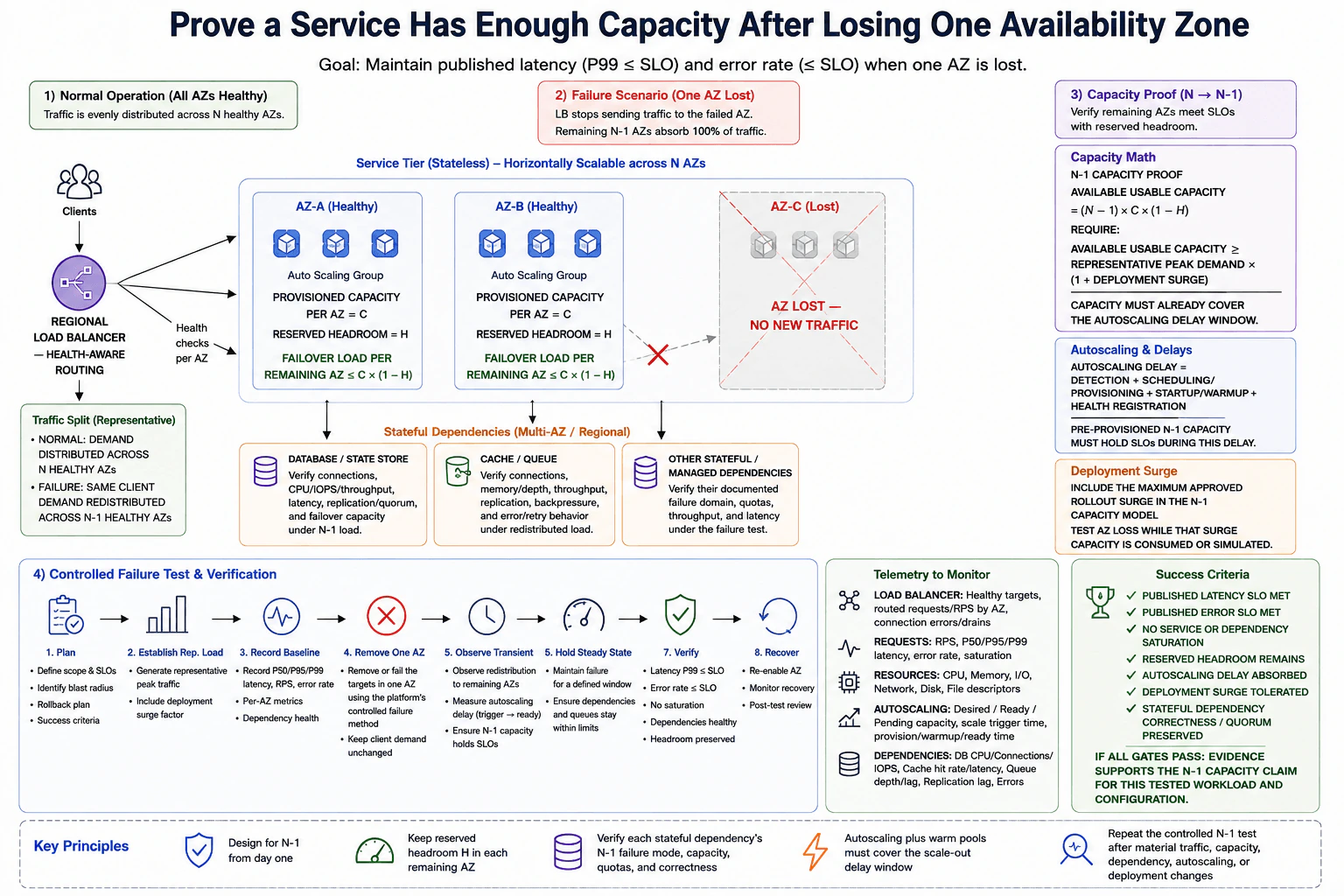
97. How would you prove that a service has enough capacity after losing one Availability Zone?Performance And CapacityHard

Question Details

A regional service is spread across multiple zones and must retain its published latency and error objectives after one zone is removed. Model normal and failure traffic distribution, reserved headroom, load-balancer behavior, stateful dependency capacity, autoscaling delay, deployment surge, and the controlled failure test and telemetry needed to verify the claim.

Short Interview Answer (30-60 seconds)

I would prove it with an N minus 1 capacity model and a controlled failure test. First, I would calculate whether the remaining zones already have enough usable capacity after reserving headroom and including deployment surge. I would also verify database, cache, queue, and other dependency limits. Then I would run representative peak demand, record a healthy baseline, remove one zone, and keep demand unchanged. I would verify load balancer redistribution, scaling delay, latency, errors, saturation, dependency health, and remaining headroom. The main tradeoff is that more reserved capacity costs more, but relying on scaling after the failure creates a risky delay window.

Detailed Explanation

The goal is to show with real evidence that the service still works well when one location that normally handles part of the traffic disappears. I first work out how much demand the remaining locations must carry and how much spare room they need. I also include extra demand caused by a software release and the time needed to add more machines. Then I run a controlled test. I remove one location while keeping demand the same and watch whether response times, failures, supporting systems, and spare capacity remain within the agreed limits.

Useful Questions to Ask the Interviewer
  1. What peak traffic level and traffic mix should the test represent?
  2. Which published latency percentile and error objective must remain satisfied?
  3. How much reserved headroom is required in each healthy zone?
  4. What deployment surge can occur while a zone is unavailable?
  5. What are the scaling detection, provisioning, startup, warmup, and readiness times?
  6. Which stateful dependencies have separate capacity, quota, quorum, or failover limits?
  7. How long should the service remain in the failure state before we accept the result?
How would you prove that a service has enough capacity after losing one Availability Zone? diagram
How to Explain It in an Interview

I would start with the capacity model. Let N be the number of healthy zones during normal operation. Let C be the provisioned capacity of each zone and H be the fraction intentionally reserved as headroom. After losing one zone, the available usable service capacity is the capacity of the remaining N minus 1 zones after reserving H. That usable capacity must be at least the representative peak demand multiplied by one plus the approved deployment surge fraction.

The important point is that I would not count future scaling capacity as immediately available. Autoscaling has a delay. Detection takes time. Scheduling or provisioning takes time. New instances or containers need startup and warmup time. They also need to become healthy before the load balancer sends traffic to them. The capacity already running in the remaining zones must keep the published latency and error objectives during this delay window.

Next, I would check the load balancer behavior. Health checks must stop new traffic from being sent to the failed zone. The same client demand should be redistributed to the remaining healthy zones. I would observe healthy target count, routed requests by zone, connection errors, and connection draining behavior. This proves that traffic really moved as expected rather than simply disappearing.

I would then check the stateful dependency boundary. Application replicas are only one part of capacity. The database or state store must have enough connections, CPU, input and output capacity, throughput, latency capacity, replication behavior, quorum behavior, and failover capacity for the redistributed load. Cache and queue systems need enough connections, memory, throughput, replication capacity, queue capacity, backpressure, and safe error and retry behavior. Other managed dependencies need enough quotas, throughput, latency capacity, and a documented failure mode that matches the test.

Deployment surge also belongs in the model. If old and new application capacity overlap during an approved rollout, that additional demand must not consume the headroom required for the zone failure. I would either run the failure test while representative rollout surge is present or simulate that surge in the capacity model and test workload.

For validation, I would first define the scope, objectives, blast radius, rollback plan, and success gates. Then I would establish representative peak demand including the traffic mix and rollout surge. While the service is healthy, I would record latency percentiles, request rate, error rate, resource use, traffic by zone, dependency health, and scaling state.

With that same demand still running, I would remove or fail the targets in one zone using the platform's controlled failure method. Client demand must remain unchanged. I would observe traffic redistribution and the complete autoscaling delay. I would then hold the service in that failure state long enough to measure steady behavior rather than judging only the first few seconds.

The test passes only if the published latency objective and error objective remain satisfied, no service or dependency becomes saturated, reserved headroom remains, the scaling delay is absorbed, deployment surge is tolerated, and stateful dependency correctness and quorum remain healthy. I would also verify that the load balancer sends new traffic only to healthy targets.

I would monitor request rate, p50, p95, and p99 latency, error rate, CPU, memory, input and output, network use, disk use, desired capacity, ready capacity, pending capacity, scaling trigger time, provisioning time, warmup time, database connections and latency, cache hit behavior, queue depth, replication lag, and dependency errors where those signals apply.

Finally, I would recover the zone and watch the system return to normal without creating another overload event. Passing the test gives evidence for the N minus 1 capacity claim for the tested workload and configuration. It is not a permanent guarantee. I would repeat the controlled test after material changes to traffic, capacity, dependencies, scaling behavior, or deployment behavior.

Technical Approach
  1. Define the published latency and error objectives and the representative peak workload.
  2. Identify N healthy zones, provisioned capacity C per zone, and reserved headroom H.
  3. Calculate the usable capacity of the remaining N minus 1 zones after reserving headroom.
  4. Include the maximum approved deployment surge in required demand.
  5. Confirm that already running capacity can hold the workload throughout scaling detection, provisioning, startup, warmup, and health registration.
  6. Check separate limits for the database, state store, cache, queue, and other managed dependencies.
  7. Establish representative peak demand and record the healthy baseline, including request metrics, traffic by zone, resources, dependencies, and scaling state.
  8. Remove one zone using a controlled platform failure method while keeping client demand unchanged.
  9. Observe load balancer redistribution and the scaling transition.
  10. Hold the failure state long enough to measure steady behavior.
  11. Verify published latency and error objectives, remaining headroom, dependency health, correctness, quorum, and absence of saturation.
  12. Recover the zone and verify stable recovery.
  13. Repeat the test after material traffic, capacity, dependency, scaling, or deployment changes.
Practical Insights

The main cost is reserved capacity. Keeping enough running capacity to survive one zone loss means some resources remain unused during normal traffic, so infrastructure cost rises. A larger deployment surge also requires more spare capacity. The controlled test consumes load testing time and engineering effort and can affect production if the blast radius is not controlled. Monitoring also needs visibility by zone and dependency. Autoscaling can reduce long term waste, but it cannot replace the capacity needed during its detection, provisioning, startup, warmup, and readiness delay.

Why Interviewers Ask This

Interviewers want to see whether I can turn a resilience claim into measurable evidence. I need to understand traffic distribution, spare capacity, dependency limits, scaling delay, rollout demand, and failure testing. They also want to see whether I check the complete regional system instead of looking only at application replicas. A strong answer shows that I define success before testing, use representative demand, observe the failure transition, verify the steady state, and use measured results rather than assumptions.

Common interview mistakes

Common mistakes include dividing normal traffic across zones and assuming the same capacity is sufficient after one zone disappears. Another mistake is counting capacity that autoscaling has not created yet. Teams may ignore startup, warmup, readiness, connection draining, or scaling detection time. They may test application replicas but forget database connections, storage throughput, cache capacity, queue depth, quotas, replication, or quorum. Other mistakes include using invented utilization thresholds, testing with unrealistic demand, removing a zone before representative load is established, changing the workload during the test, checking only average latency, ignoring deployment surge, stopping the test before steady state, and declaring permanent resilience from one successful run.

Interview tip

Explain the proof in three parts. First show the N minus 1 capacity model with reserved headroom, deployment surge, and scaling delay. Second explain how traffic and stateful dependencies behave when one zone disappears. Third describe the controlled test and the exact telemetry and pass gates. Make it clear that autoscaling is helpful after failure but is not instant capacity. Finish by saying that a passing test supports the capacity claim for the tested workload and configuration rather than guaranteeing every future workload.

Interviewer may ask next
What if the service has low CPU after the zone failure but p99 latency still violates the objective?

I would not conclude that the service has enough capacity from CPU alone. The exact workload is the same representative peak demand running after one zone is removed. The measurement boundary includes the load balancer, application capacity, database or state store, cache, queue, network, and other dependencies. I would check request distribution by zone, connection limits, database latency, input and output saturation, queue depth, replication lag, network behavior, and pending capacity. A hidden dependency or connection limit can increase p99 latency while application CPU remains low. The tradeoff is that broader telemetry requires more instrumentation, but it prevents a false capacity conclusion.

Would you reduce reserved headroom if autoscaling becomes much faster?

Possibly, but only after repeating the same N minus 1 capacity test with measured scaling behavior. The workload remains the representative peak demand plus the approved deployment surge, and the measurement boundary still includes the remaining zones and all stateful dependencies. Faster detection, provisioning, startup, warmup, and readiness can reduce the amount of capacity needed for the transition, but scaling is still not instantaneous and dependencies may have fixed limits. I would change headroom only if repeated tests show that published latency and error objectives remain satisfied throughout the failure window with no saturation or correctness problem. The tradeoff is lower infrastructure cost versus less protection from traffic variation, scaling delay, or dependency slowdown.

98. Where should unit, integration, and end-to-end tests run in a delivery pipeline?Testing And Release ValidationEasy

Question Details

Map each test type to the earliest useful release stage and explain its scope, dependencies, speed, isolation, and failure signal. Define which failures block artifact creation, environment deployment, or production promotion, and why a passing end-to-end suite does not replace lower-level tests.

Short Interview Answer (30-60 seconds)

I would run unit tests first, before creating or publishing the release artifact. They are fast and isolate small pieces of code. After they pass, I would create the artifact and run integration tests with controlled real dependencies. An integration failure blocks deployment to staging or pre prod. After that artifact is deployed to a realistic environment, I would run end to end tests. An end to end failure blocks production promotion. I keep all three levels because lower level tests are faster and give clearer failure signals.

Detailed Explanation

The safest approach is to check small pieces first, then check groups of parts working together, and finally check the whole product before it reaches real users. Each check should happen as early as it can give useful information. If an early check fails, the next risky action should stop. This saves time because simple problems are found quickly. Later checks give broader confidence because they use more of the real product. Together, these checks make releases faster to diagnose and safer to promote.

Useful Questions to Ask the Interviewer
  1. Does the pipeline create one artifact and promote that same artifact through later environments?
  2. Which real services are available to integration tests in the controlled test environment?
  3. Is staging or pre prod close enough to production for the main user journeys to be meaningful?
Where should unit, integration, and end-to-end tests run in a delivery pipeline? diagram
How to Explain It in an Interview

I would organize the pipeline as code commit, build and compile, unit test, package and create the artifact, integration test, deploy to staging or pre prod, end to end test, and then production promotion.

Unit tests run first. Their boundary is one small function, class, or module. External systems stay outside that boundary. I use mocks or stubs where needed so network services, databases, queues, and other outside systems do not make the test slow or unpredictable. The setup uses small deterministic inputs. The test runs one behavior and checks its visible result. Typical failures point to logic, validation, or edge case problems. Unit tests are usually very fast and highly isolated. If they fail, the pipeline must stop before packaging or publishing the release artifact.

After unit tests pass, the pipeline creates and publishes the artifact that later stages will validate. Integration tests then check whether selected components work correctly with controlled real dependencies. Depending on the application, these dependencies can include a database, cache, API, or message queue. The boundary is wider than a unit test, so isolation is lower and setup costs more. Test data should be created specifically for the run. Shared state should be reset or removed afterward. Assertions should focus on contracts, configuration, data behavior, and connectivity. If integration tests fail, deployment to staging or pre prod must stop.

The artifact that passed the earlier gates is then deployed to a realistic staging or pre prod environment. Smoke or health checks can confirm that the deployment is available before longer validation begins. End to end tests run after this deployment because the full application and its important real dependencies must already be available. Their boundary is a complete user journey through the deployed system. They are slower and less isolated. Failures can point to workflow, user experience, data integrity, configuration, routing, or integration problems. If the required end to end suite fails, production promotion must stop.

A passing end to end suite does not replace unit or integration tests. End to end tests give broad confidence, but they are slower and usually give a less precise failure signal. They can also fail because of environment or test data problems. They cannot practically cover every small logic branch and edge case. Unit tests catch isolated defects quickly. Integration tests expose contract and dependency problems before the full environment is involved. All three levels are useful because each finds a different class of problem at the earliest useful stage.

For reliability, each level should use deterministic test data and should not depend on test execution order. Unit tests should control outside dependencies. Integration tests should use controlled infrastructure and reset state between runs. End to end tests should focus on important user journeys instead of trying to cover every possible case. Cleanup should remove or reset created data when an environment is reused. CI should stop when a required gate fails so an unverified artifact cannot move to the next protected stage.

Technical Approach
  1. Build or compile the committed code and run basic static checks.
  2. Run unit tests against small isolated code boundaries with outside dependencies replaced where needed.
  3. If unit tests fail, stop before packaging or publishing the artifact.
  4. If unit tests pass, package and publish the artifact that later stages will validate.
  5. Run integration tests using selected real dependencies in a controlled environment.
  6. If integration tests fail, stop before deployment to staging or pre prod.
  7. Deploy the tested artifact to staging or pre prod and run basic smoke or health checks.
  8. Run focused end to end tests across important complete user journeys.
  9. If end to end tests fail, block production promotion.
  10. If the required gates pass, promote the verified artifact to production.
Practical Insights

Traditional algorithm complexity does not apply to this question. The important costs are test runtime, environment setup, test data setup, cleanup, and maintenance. Unit tests are usually cheapest because they run with isolated dependencies and often finish in milliseconds or seconds. Integration tests cost more because real services, processes, containers, databases, or network boundaries may need setup and cleanup. End to end tests usually cost the most because a realistic deployed environment must be available and complete user journeys take longer. Keeping detailed checks at lower levels reduces CI time, infrastructure cost, and debugging time.

Why Interviewers Ask This

Interviewers want to see whether I can place each test type at the earliest useful point in a delivery pipeline. They are checking whether I understand test scope, isolation, real dependencies, failure diagnosis, and release gates. A strong answer shows that I know which failures should stop artifact creation, which failures should stop deployment to a test environment, and which failures should stop promotion to production.

Common interview mistakes

Common mistakes include creating or publishing the release artifact before required unit tests pass, using only end to end tests for every type of defect, and calling a test an integration test when all important dependencies are mocked. Another mistake is allowing an integration failure to continue into staging deployment. Teams can also make end to end suites too large, which creates slow feedback and difficult diagnosis. Shared mutable test data can cause flaky results. Tests should not depend on execution order or uncontrolled external state. A passing end to end suite should not be treated as proof that every small logic branch, dependency contract, or edge case is correct.

Interview tip

Explain the pipeline from left to right and connect each test level to one release gate. Say that unit failures stop artifact creation, integration failures stop staging or pre prod deployment, and end to end failures stop production promotion. Then explain why the levels complement each other. Lower level tests are faster and easier to diagnose, while the final level gives broader confidence in the deployed system.

Interviewer may ask next
What would you do if end to end tests become flaky because the shared staging environment or test data changes during the run?

I would keep the end to end boundary at the deployed staging or pre prod environment, but I would make its data and observable conditions more controlled. I would create unique test data for each run, avoid depending on execution order, clean up created state, and wait for observable conditions with bounded time limits instead of fixed sleeps. If unrelated shared activity still causes failures, I would reduce shared state or use a more isolated environment for critical journeys. The tradeoff is higher environment cost in exchange for a more reliable production promotion signal.

What would you change if the end to end suite becomes so slow that it delays every production release?

I would keep end to end tests as the production promotion boundary, but reduce that suite to the most important complete user journeys. Detailed logic and edge cases should remain in unit tests, while component contracts and real dependency behavior should remain in integration tests. This moves more feedback into faster stages without removing the final system level gate. I could also run independent end to end scenarios in parallel when the environment safely supports it. The tradeoff is that a smaller final suite provides less broad coverage, so lower level tests must carry more detailed validation.

99. What is a CI/CD quality gate?Testing And Release ValidationEasy

Question Details

A pipeline collects test, coverage, security, and policy results before promotion. Define a deterministic gate with named inputs, thresholds or required statuses, ownership of exceptions, behavior when evidence is missing, and the exact release transition that a pass or fail permits.

Short Interview Answer (30-60 seconds)

I would make the quality gate a deterministic checkpoint before promotion. It receives named evidence such as test results, code coverage, security results, policy checks, and evidence freshness. Each input has a required status or threshold. In this example, the test pass rate must be at least 98 percent, line coverage must be at least 80 percent, there can be no High or Critical vulnerabilities, all mandatory policies must pass, and all results must be less than 24 hours old. If every rule passes, the artifact can move to staging. If any rule fails or required evidence is missing, promotion is blocked. Exceptions require a designated owner, a recorded reason and reference, an approver, and an expiry.

Detailed Explanation

A quality gate is a clear checkpoint before a software release moves forward. The pipeline gathers evidence about the build, such as test results, coverage, security results, and policy results. It compares every required result with a fixed rule. The same evidence should always produce the same decision. If every rule passes, the artifact may move to staging. If one rule fails or required evidence is missing, promotion stops. Any exception must have an approved owner, a recorded reason, and an expiry so the decision stays controlled and traceable.

Useful Questions to Ask the Interviewer
  1. Which evidence is required before promotion?
  2. What thresholds and required statuses should the gate use?
  3. Is staging the exact next release stage controlled by this gate?
  4. Who may approve an exception, and how long may it remain valid?
What is a CI/CD quality gate? diagram
How to Explain It in an Interview

I would start by defining the boundary. The quality gate does not perform every test or scan itself. Earlier pipeline jobs produce the evidence. The gate reads that evidence and decides whether the artifact may be promoted.

The named inputs in this design are test results, code coverage, a security scan result, policy check results, and evidence freshness. The rules are explicit. The test pass rate must be at least 98 percent. Line coverage must be at least 80 percent. The security result must show no High or Critical vulnerabilities. Every mandatory policy must pass. All required results must also be less than 24 hours old.

The gate checks every required input against its rule. All rules must pass for the gate to return PASS. Because the rules are fixed and versioned, the same evidence and the same rule version should produce the same result. This makes the release decision deterministic.

A PASS has one exact release meaning in this design. It allows the artifact to move to staging, which is the next release stage. Passing this gate does not automatically approve production. A later stage may have its own validation and approval rules.

A FAIL blocks promotion. The artifact remains in its current stage. The pipeline should show the failed rule, notify the team, and require the relevant problem to be corrected before validation is run again.

Missing evidence also causes a FAIL. If a required result is missing, unavailable, or timed out, promotion remains blocked until valid evidence exists. This is safer than treating an unavailable test or scanner as a successful check.

Exceptions are controlled outside the normal automatic PASS path. Only designated exception owners may approve them. The exception record should include the reason, a ticket or other reference, the approver, and an expiry. Exceptions should be time limited and auditable so a temporary decision does not silently become permanent policy.

The main tradeoff is release safety versus pipeline speed. More checks and stricter thresholds can reduce release risk, but they also add execution time and can block releases when rules are poorly chosen. The better approach is to measure the value of each rule, version rule changes, and use controlled exceptions only when there is a documented reason.

Technical Approach
  1. Collect the named evidence for the artifact: test results, code coverage, the security scan result, policy check results, and freshness information.
  2. Verify that every required input exists and is valid. If required evidence is missing, unavailable, or timed out, return FAIL and block promotion.
  3. Check that the test pass rate is at least 98 percent.
  4. Check that line coverage is at least 80 percent.
  5. Check that the security result contains no High or Critical vulnerabilities.
  6. Check that all mandatory policies pass.
  7. Check that all required results are less than 24 hours old.
  8. Return PASS only when every rule passes. PASS allows promotion of the artifact to staging.
  9. If any rule fails, return FAIL, keep the artifact in its current stage, show the failed rule, notify the team, and run the relevant validation again after correction.
  10. Handle any approved exception through a designated owner and record the reason, reference, approver, expiry, and audit history.
Practical Insights

Traditional algorithmic complexity is not important for this question. The gate itself reads a small set of validation results and compares them with fixed rules, so the decision step is inexpensive. Most pipeline time comes from producing the evidence, such as running tests, measuring coverage, scanning for vulnerabilities, and evaluating policies. Adding more required checks increases pipeline duration and maintenance work. A freshness rule can also force expensive checks to run again when results become too old. The main operational cost is keeping rules, evidence formats, and exception records accurate and reliable.

Why Interviewers Ask This

Interviewers ask this to see whether I can turn validation evidence into a clear release decision. They want to know whether I can name the required inputs, define measurable rules, handle missing results safely, control exceptions, and state exactly what a pass or fail allows. It also tests whether I understand that a release gate should give the same decision for the same evidence and rules instead of depending on manual judgment during each pipeline run.

Common interview mistakes

A common mistake is treating the quality gate as a vague manual review instead of defining exact inputs and rules. Another mistake is allowing missing evidence to count as success. Teams may also treat coverage as proof that the software is correct even though coverage only shows which code was exercised. Other problems include unclear security severity rules, accepting stale evidence, changing thresholds without version control, and allowing exceptions with no owner or expiry. A PASS should also map to one exact transition. In this design, PASS permits promotion to staging. It does not automatically permit production deployment.

Interview tip

Explain the gate as a simple sequence: collect named evidence, apply fixed rules, make one deterministic PASS or FAIL decision, and connect that decision to an exact release transition. Then mention missing evidence and exception ownership because those details show practical production judgment.

Interviewer may ask next
What should the quality gate do if the security scan service times out and produces no result?

The gate should return FAIL because the required security evidence is missing. The boundary here is the gate decision, not the internal behavior of the scanner. The gate only knows that a required input is unavailable. It should block promotion to staging, keep the artifact in the current stage, identify the missing evidence, and run the relevant validation again when the scanner is available. This matters because treating an unavailable check as success could promote an artifact without required security evidence. A designated owner may use the controlled exception process only when policy permits it and the reason, reference, approver, and expiry are recorded.

What tradeoff would you consider when adding more checks or stricter thresholds to this gate?

I would keep the same gate boundary but review whether each additional rule reduces enough release risk to justify its pipeline cost. More tests, scans, policies, or stricter thresholds can increase confidence, but they can also increase pipeline time and create unnecessary release blocks when a rule is poorly calibrated. The gate should remain deterministic and should still return FAIL when a required rule fails or evidence is missing. I would measure the effect of the proposed rule, version the rule change, and keep the PASS transition as promotion to staging.

100. What should a deployment smoke test verify?Testing And Release ValidationEasy

Question Details

Immediately after deployment to a target environment, define a fast blocking suite that proves the application starts, is reachable, serves one critical workflow, and can contact essential dependencies. State the allowed test data, timeout, pass or fail rule, evidence captured on failure, and whether promotion or rollback follows.

Short Interview Answer (30-60 seconds)

I would run a fast blocking smoke test immediately after deployment. It should verify that the application starts, is reachable, completes one critical user workflow, and can contact the essential dependencies it needs. I would use dedicated safe smoke data and give the whole suite a short timeout, such as 60 seconds. Every required check must pass. If they all pass, the pipeline can promote or continue the release. If any check fails or times out, I would block promotion, capture evidence, and roll back or disable the release.

Detailed Explanation

A deployment smoke test is a small safety check that runs right after a new version is placed in the target environment. Its job is to answer a simple question: is this version healthy enough to continue? It checks that the application is running, people can reach it, one important action works from start to finish, and the services it depends on can be contacted. The test should use safe dedicated data, finish quickly, save useful failure information, and stop the release when any required check fails.

Useful Questions to Ask the Interviewer
  1. Which user workflow is the most important one to validate after deployment?
  2. Which external services are considered essential for this release?
  3. Should a failed smoke test automatically roll back the deployment or only block promotion?
  4. What total smoke test timeout does the release pipeline expect?
What should a deployment smoke test verify? diagram
How to Explain It in an Interview

The system under test is the newly deployed application in the target environment, such as staging or production. This is deployment validation against the real deployed version, not an isolated unit test. The purpose is to detect a bad release quickly before it is promoted further or receives more traffic.

I would make the smoke suite fast and blocking. The diagram uses four required checks. First, verify that the application starts and that its health endpoint responds successfully. The example uses GET /health with a 5 second timeout. Second, verify that the service is reachable through the expected network path, including TLS and HTTPS. The example uses GET / with a 5 second timeout. Third, run one critical workflow. The example creates an item with POST /items and then reads it with GET /items/{id}, with a 10 second timeout. Fourth, verify essential dependencies. The example checks the database with a simple read query, the cache with a ping, the queue or messaging path with a dry run publish, and an external API with a heartbeat. These dependency checks use a 5 second timeout each.

The smoke test uses dedicated smoke test data. The data should be read only where possible or temporary when a write is required. It must not depend on real user data. If the critical workflow creates temporary data, the test should remove it when practical so repeated runs remain predictable.

The checks run immediately after deployment through the CI/CD pipeline. The complete suite has a 60 second budget in the diagram. Each individual check also has a smaller bounded timeout. The runner should fail quickly when a required check fails or reaches its timeout instead of waiting unnecessarily.

The pass rule is strict. All required checks must succeed within the allowed time and return the expected result. A partial pass is still a failed smoke test. A timeout, an unreachable dependency, an unhealthy application, or a broken critical workflow should block promotion.

When the suite passes, the deployment can be promoted, the rollout can continue, traffic can be opened as appropriate, and the release can be marked healthy. When the suite fails, the pipeline blocks promotion. The release process should stop the rollout, roll back or disable the failed release according to the deployment mechanism, and notify the responsible team.

Failure evidence is important because the smoke test must help engineers understand why the release failed. The diagram captures smoke test request and response details, status and latency information, HTTP status codes and error messages, application or pod logs around the failure time, dependency error details, and CI/CD artifacts. The process should also alert the responsible team when the release gate fails.

The important tradeoff is speed versus coverage. A smoke test checks only a few high value paths. It is not a replacement for the full test suite. Its value is that it runs against the real deployed environment and quickly catches problems such as a process that did not start, a routing or TLS problem, a broken critical workflow, or incorrect dependency wiring.

Technical Approach
  1. Deploy the new version to the target environment.
  2. Start the automated smoke test immediately after deployment.
  3. Verify that the application starts and that GET /health succeeds within 5 seconds.
  4. Verify that the service is externally reachable and that GET / succeeds through the expected TLS and HTTPS path within 5 seconds.
  5. Run the critical workflow by creating an item with POST /items and reading it with GET /items/{id}, with a 10 second timeout.
  6. Verify essential dependencies with the example checks shown in the diagram: a database read query, cache ping, queue or messaging dry run publish, and external API heartbeat, using a 5 second timeout for each dependency check.
  7. Use only dedicated smoke test data that is read only or temporary and does not use real user data.
  8. Keep the complete suite within the 60 second release budget and fail quickly on the first hard failure or timeout.
  9. Collect the smoke test results, status and latency information, HTTP errors, application or pod logs, dependency errors, and CI/CD artifacts.
  10. Pass only when every required check succeeds within its timeout and returns the expected result.
  11. On success, promote or continue the rollout and mark the release healthy. On failure, block promotion, stop the rollout, roll back or disable the failed release, and notify the responsible team.
  12. Remove temporary test data when the workflow creates state.
Practical Insights

Algorithmic complexity is not the useful measure for this smoke test. The important cost is release time and operational work. The diagram keeps the complete suite within 60 seconds, with smaller time limits for each check. Network calls, application response time, dependency checks, and the critical workflow usually dominate the runtime. Safe test data may also need setup and cleanup. Adding too many checks increases CI duration and maintenance cost, so the suite should contain only the small set of checks needed to decide whether the deployment is safe to continue.

Why Interviewers Ask This

Interviewers ask this to see whether I can design a small release gate that quickly detects a broken deployment without trying to run the full test suite. They want to see whether I understand what must be checked in the deployed environment, how to use safe test data, how to set strict timeouts, what evidence to save when something fails, and when the pipeline should promote the release or roll it back.

Common interview mistakes

Common mistakes include turning the smoke suite into a large regression suite, checking only that a process exists without testing reachability, skipping the critical workflow, or failing to validate essential dependencies. Another mistake is using real customer data instead of dedicated smoke data. Teams may also use long waits, weak timeout rules, or retries that hide a real release problem. A weak pass rule can allow partial success to promote a broken release. Other mistakes include capturing too little failure evidence, leaving temporary test data behind, treating the smoke test as proof that every feature works, or allowing the pipeline to continue after a required smoke check fails.

Interview tip

Explain the smoke test as a fast blocking release gate. Start with the four things it must prove: the application starts, it is reachable, one critical workflow works, and essential dependencies are available. Then state the safe data rule, the bounded timeouts, the all checks must pass rule, the evidence captured on failure, and the final decision: promote or continue on success, or block and roll back or disable the release on failure.

Interviewer may ask next
What should happen if the application is healthy and reachable but the critical workflow times out?

The smoke test should fail and block promotion. The exact boundary is the deployed critical workflow, not only the application health check. A healthy process does not mean the release is usable. I would capture the request and response details, status and latency information, HTTP errors, application or pod logs, dependency errors, and CI/CD artifacts. The release process should stop the rollout and roll back or disable the failed release according to the deployment mechanism. The main tradeoff is that a strict gate may stop a release because of a temporary problem, but allowing a broken critical path to continue creates a larger release risk.

How would you keep deployment smoke tests fast as the application grows?

I would keep the test boundary limited to release critical behavior. I would continue checking application startup, external reachability, one representative critical workflow, and only the dependencies needed for basic service operation or that workflow. Each check would keep a bounded timeout, and the complete suite would stay within the release budget. Broader functional coverage should remain in earlier or separate test stages. The tradeoff is lower coverage in the smoke suite, but that keeps the deployment gate fast enough to give useful feedback immediately after release.

More questions load as you scroll

Disclaimer: This interview guide is for educational and informational purposes only. It is designed to help readers prepare, but it does not guarantee any interview result, hiring decision, offer, or outcome. Interview questions, hiring criteria, and preferred answers can vary by employer, interviewer, industry, location, and time. The examples and explanations reflect the authors' research and judgment, are provided without warranties of any kind, and should not be treated as the only correct approach. Diagrams are simplified illustrations intended to highlight the main components and their interactions; actual systems and implementations may be more complex. Alternative approaches may be equally valid or better suited to a particular question, context, or interviewer. To the fullest extent permitted by applicable law, the author, contributors, and publisher are not liable for decisions made, actions taken, or losses incurred based on this guide.

Content Accuracy and Verification: To the fullest extent permitted by applicable law, we do not represent or warrant that interview guides, questions, answers, examples, or diagrams are accurate, complete, current, error-free, or suitable for any particular purpose. You are responsible for independently reviewing and verifying the information before relying on it.